Matsumoto_unc_0153D_15284.pdf

(1)

E

STIMATING

M

ODELS OF

L

EARNING IN

I

NDIVIDUAL

D

ECISION MAKING WITH

AN

A

PPLICATION TO

Y

OUTH

S

MOKING

Brett Matsumoto

A dissertation submitted to the faculty of the University of North Carolina at Chapel Hill in par-tial fulfillment of the requirements for the degree of Doctor of Philosophy in the Department of

Economics.

Chapel Hill 2015

Approved by:

Donna Gilleskie

Peter Arcidiacono

Clement Joubert

Brian McManus

(2)

c

2015

(3)

ABSTRACT

BRETT MATSUMOTO: Estimating Models of Learning in Individual Decision making with an Application to Youth Smoking.

(Under the direction of Donna Gilleskie)

In the first chapter of my dissertation, I examine the dynamics of youth smoking behavior using

a model of rational addiction with learning. Individuals in the model face uncertainty regarding the

parameters that determine their utility from smoking. Through experimentation, individuals learn

about how much they enjoy smoking cigarettes as well as the effects of reinforcement, tolerance, and

withdrawal. The addition of learning to the dynamic optimization problem of adolescents provides

an explanation for the experimentation of the non-smoker. I estimate the parameters of the model

using data from the National Longitudinal Survey of Youth 1997 and compare the overall fit of the

model to the model without learning. The estimated model is also used to analyze the effect of

cigarette taxes and anti-smoking policies. I find that the model with learning is better able to fit the

observed data and that cigarette taxes are not only effective in reducing the level of youth smoking,

but can even increase welfare for some individuals.

In the second chapter (with Jonathan James), we show how the conditional choice probability

(CCP) estimation procedure of Arcidiacono and Miller (2011) can be extended to feasibly estimate

structural learning models. Although the focus of the paper is the specific application to learning

models, the procedure could be used to estimate any model with continuous unobserved

hetero-geneity. Monte-Carlo simulations show that the CCP method can provide significant computational

savings relative to Simulated Maximum Likelihood.

In the third chapter (with Forrest Spence), we investigate whether an individual’s subjective price

beliefs reflect the empirical distribution of prices and whether an individual learns about features of

the price distribution through experience in the market. We use data on subjective price beliefs from

(4)

prices to be higher than what is observed empirically. However, consumers with more experience in

the marketplace generally have more accurate beliefs about the price distribution, which is consistent

(5)

ACKNOWLEDGMENTS

I have benefitted greatly from the advice and support of many people. I would like to thank my

advi-sor Donna Gilleskie and committee members Peter Arcidiacono, Clement Joubert, Brian McManus,

and Helen Tauchen. I would also like to thank Wayne-Roy Gayle, Juan Pantano, Tiago Pires, Steven

Stern, and the UNC Applied Microeconomics Workshop for helpful comments and suggestions.

Ad-ditionally, conversations and discussions with Forrest Spence, Matt Harris, and many other graduate

(6)

LIST OF TABLES

1.1 Individual Level Survey Participation . . . 14

1.2 Categorical Smoking Statistics . . . 15

1.3 Cumulative Smoking Transition Probabilities . . . 16

1.4 Under 18 Smoking Transition Probabilities . . . 16

1.5 Summary Statistics of Smoking and Demographic Variables in Select Years . . . 18

1.6 Summary Statistics of State Tobacco Price and Taxes . . . 20

1.7 Estimation Results, Population Distribution Parameter Estimates . . . 31

1.8 Estimation Results, Coefficients on Observable Variables . . . 32

1.9 Transition Probabilities, Observed and Simulated Data . . . 34

1.10 Welfare Analysis . . . 42

2.1 Naive learning model Monte Carlo results forN = 100andK = 0 . . . 57

2.7 Full learning model Monte Carlo results forK = 0 . . . 63

2.8 Full learning model Monte Carlo results forK = 1 . . . 64

3.1 Respondent Characteristics . . . 86

3.2 Ratio of Amazon Prices to Bookstore Prices by Survey Period . . . 86

3.3 Mean Ratio Comparisons by Online Purchasing Experience, Used Books . . . 87

3.4 Mean Difference Comparisons by Online Purchasing Experience, Used Books . . . . 87

(11)

3.6 (Online Expectation / Bookstore Price) Regressed on Prev. Purchases . . . 89

3.7 (Online Expectation / Bookstore Price) Regressed on Experience . . . 90

3.8 Reported Probability that Lowest Price< b∗Expected Lowest Price . . . 90

3.9 Mean and Variance Comparisons (Log-Normal Assumption) . . . 91

3.10 Mean Comparison by Major . . . 92

3.11 Variance Comparison by Major (Log-Normal Assumption) . . . 92

3.12 Parameter Values by Change in Experience . . . 93

A.1 Summary statistics by year for individuals observed every period . . . 95

B.1 Textbook Scenarios . . . 109

B.2 Survey Attrition . . . 110

B.3 Results Using Alternative Samples . . . 111

(12)

LIST OF FIGURES

1.1 Smoking Choice Probabilities by Age . . . 19

1.2 Gender and Racial Differences in Smoking Rates by Age . . . 19

1.3 Real Cigarette Taxes and Prices in NY and NC (in year 2000 dollars) . . . 22

1.4 Distribution of Real State Cigarette Taxes by Year . . . 22

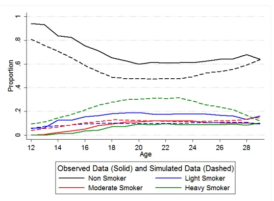
1.5 Smoking Rates by Age, Observed and Simulated Data from the Model with Learning 34 1.6 Smoking Rates by Age, Observed and Simulated Data from Model without Learning 36 1.7 Experimentation Rates by Age, Observed and Simulated Data from Model with Learning . . . 36

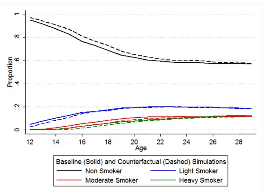
1.8 Smoking Rates by Age, Baseline Simulation and Price Counterfactual Data . . . 38

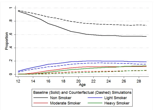
1.9 Smoking Rates by Age, Baseline Simulation and Beliefs Counterfactual Data . . . . 38

1.10 Smoking Rates by Age, Baseline Simulation and Smoking Age Counterfactual Data . 40 1.11 Experimentation Rates by Age, Baseline Simulation and Counterfactual Data . . . . 40

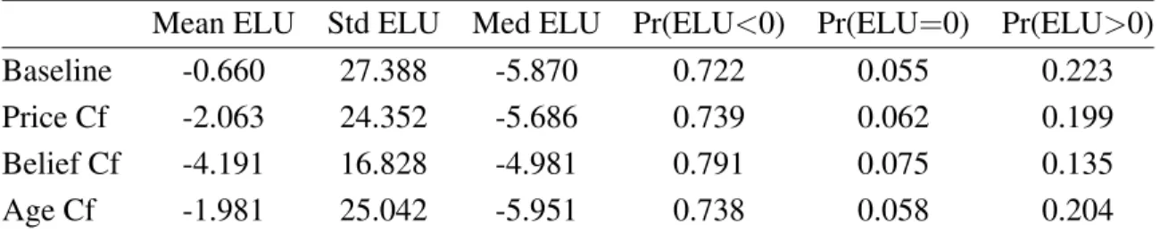
1.12 Distribution of Expected Lifetime Utility . . . 41

3.1 Textbook Purchasing Scenario . . . 85

3.2 Used price pdf versus empirical dist. by level of experience . . . 88

3.3 New price pdf versus empirical dist. by level of experience Newalt is the minimum price for a new textbook from Amazon or Amazon Marketplace. . . 89

B.1 Histograms of Prices . . . 114

B.2 Kernel Density Estimate . . . 115

B.3 Kernel Density Estimate . . . 115

B.4 Daily Used Prices . . . 116

(13)

CHAPTER 1

EXPLAINING YOUTH SMOKING INITIATION IN THE CONTEXT OF A RATIONAL ADDITION MODEL WITH LEARNING

1.1 Introduction

Despite its historically low level in the U.S., cigarette smoking remains a major public health

concern. The Surgeon General estimates that tobacco use causes approximately 480,000 deaths per

year in the United States and is estimated to cause between $289-332.5 billion in economic costs

(USDHHS 2013).1 Tobacco use is the leading preventable cause of death, yet people continue to

smoke despite the high level of public awareness of its adverse health effects. Because cigarettes

are addictive, it may be easier to discourage smoking initiation than to encourage smoking

cessa-tion. Also, cigarette manufacturers have historically targeted their advertisements to young people

in the hopes of cultivating lifelong customers. Among adults who become daily smokers,

approxi-mately 90 percent smoke for the first time before age 18 (USDHHS 2012). For these reasons, policy

interventions aimed at reducing the level of smoking in the population often target young people.

The decision to engage in a harmful addictive behavior, such as smoking, seemingly presents

a problem for standard economic models. Consuming a harmful addictive substance would be an

irrational act for a forward-looking utility-maximizing agent. The Rational Addiction (RA) model

of Becker and Murphy (1988) shows that consumption of an addictive substance can be explained

using the standard economic framework. Their explanation of addictive behavior centers around the

concept that past utilization of addictive goods impacts current utility from consumption of these

goods. A major criticism of the Becker and Murphy model is the implication that individuals are

always acting optimally, so addicts do not regret their decision to consume the addictive good. In

1_{Economic costs include direct medical costs in addition to the lost productivity attributable to smoking related}

(14)

their model addiction is not a problem or even an undesirable outcome, so there is no place for policy

intervention to treat or prevent addiction. Empirical evidence suggests that many individuals regret

their decision to smoke. Approximately 70% of adult smokers wish to quit smoking entirely and

over half have attempted to quit smoking in the past year (NHIS, 2010).

Another limitation of the RA model as a model of youth smoking behavior is that it treats

smok-ing initiation as exogenous. In this paper, I extend the RA model so that it is better able to explain the

individual’s smoking initiation decision. Specifically, I relax the assumption of perfect information

in the RA model by incorporating learning about one’s preferences. The parameters that determine

the utility one receives from smoking are initially unknown, but the individual has beliefs about their

true value. As an individual experiments with smoking, he receives utility signals and updates his

beliefs. The addition of uncertainty and learning to the optimization problem of adolescents

pro-vides an explanation for the experimentation of the non-smoker and allows for the possibility that

an individual who starts to smoke may later regret that decision. Therefore, policies that prevent an

individual from experimenting with cigarettes may be welfare improving as the individual would be

prevented from making a decision he may later regret.

The main purpose of this paper is to quantify the effectiveness of anti-smoking policies and to

evaluate the resulting impact on individual welfare. In order to do this, I recover the policy-invariant

utility function parameters of a rational addiction model with learning by fitting a dynamic discrete

choice model of optimal smoking decision making to the observed data. As the first attempt to

estimate the structural parameters of a rational addiction model with learning about preferences, this

research allows for empirical testing of the perfect information assumption in the RA model (i.e., the

assumption that individuals know their utility function parameters). I estimate the model parameters

using the National Longitudinal Survey of Youth 1997 (NLSY97).

Estimation of the parameters of a dynamic discrete choice model is generally computationally

intensive as each iteration over the parameter space requires re-solving the dynamic optimization

problem. The inclusion of uncertainty and learning over multiple parameters further complicates

estimation of the model. To circumvent these computational issues, I use the Expectation

(15)

Monte Carlo simulation to estimate the model parameters. The estimation procedure provides a

sig-nificant computational advantage, which allows for the estimation of a more complex model than is

feasible using full-solution techniques.

Preliminary estimation results demonstrate that allowing for uncertainty and learning in a

dy-namic model of youth smoking significantly improves the overall fit of the model. Results from

counterfactual policy simulations suggest that policies that impact individuals’ initial beliefs about

their utility function parameters are effective in reducing youth smoking. Taxes are also shown to

be effective in reducing the level of smoking. The estimated model predicts that a doubling of the

price of cigarettes would reduce the prevalence of youth smoking by 12.3% and adult smoking by

12.6%. An increase in the legal purchasing age from 18 to 19 years old would decrease youth

smok-ing by 21.7%. However, there would be no effect on adult smokers as the higher legal purchassmok-ing

age would only cause a delay in smoking initiation. The results of the welfare analysis show that

increasing cigarette taxes would only lead to a relatively small loss in total welfare as the welfare

gains to keeping those who would later regret the decision to smoke from starting to smoke offset

the loss of welfare from smokers having to pay a higher price for cigarettes.

The remainder of the paper proceeds as follows: Section 2 reviews the related literature. Section

3 presents the model. Section 4 discusses the data. Section 5 develops the estimation routine. The

estimation results are presented in section 6, and section 7 concludes.

1.2 Related Literature

Becker and Murphy (1988) developed the RA model to show that seemingly irrational behavior

could be explained using a standard economic framework of a forward-looking utility-maximizing

agent. The model’s welfare implications have caused many to abandon the general framework of the

RA model and to develop “irrational” models to explain the time inconsistency of addictive behavior.

These alternative theoretical models generally feature dual-states of the world or individuals with

dual-selves.2 Addiction results when an individual is in an addictive state of the world or if the

behavior of the individual is being controlled by the self that is more prone to addiction.

2_{Papers that use the dual-state approach include Winston (1980) and Bernheim and Rangel (2004). Papers that use}

(16)

Other models of the consumption of addictive goods generate time-inconsistent behavior by

de-viating from the standard assumptions regarding how future utility is discounted. The simplest

devia-tion is the myopic model. A myopic individual completely discounts future utility and only considers

the current period’s utility when making decisions. Other deviations from the standard assumptions

regarding time preferences include an endogenous discount factor (Orphanides and Zervos 1998) or

hyperbolic discounting (Gruber and Koszegi 2001). Finally, Orphanides and Zervos (1995) argue

that the problem with the RA model is not the assumption of a rational, forward-looking agent but

the assumption of perfect information. An individual in their model can be one of two types (addict

or not an addict). The individual learns which type he is if he consumes the addictive good. The

model estimated in this paper is an extension of the theoretical model proposed by Orphanides and

Zervos (1995).

The RA model assumes that individuals are forward-looking, and there have been many studies

that attempt to test the validity of this assumption empirically in the context of consumer demand

for an addictive good. The evidence is generally consistent with forward looking behavior (Becker,

Grossman, and Murphy 1994; Chaloupka 1991).3 _{One of the limitations of the empirical addiction}

literature is that papers primarily attempt to compare the rational addiction model to the myopic

model. No work (of which the author is aware) has been done to estimate alternative models or

to empirically test the other assumptions of the RA model. Most of the literature involves reduced

form estimation, but a few papers have estimated the structural parameters of an addiction model

(Arcidiacono, Sieg, and Sloan 2007; Choo 2000; Gordon and Sun 2009; Darden 2011).4

Much of the analysis in the economics literature of policy interventions on youth smoking has

focused on cigarette taxes. The rational addiction framework implies that individuals who are not

currently consuming the addictive good should be more responsive to changes in the price of that

good than current users. Many studies have found a significant effect of taxes on smoking initiation.

Some studies, however, have found that cigarette taxes have little to no significant effect on youth

3_{See Chaloupka and Warner (2000) for a thorough summary of the empirical literature.}

4_{There is a learning component to the life-cycle model of Darden (2011), but the learning is over the health effects of}

(17)

smoking initiation (DeCicca, Kenkel, and Mathios 2002; DeCicca, Kenkel, Mathios, Shin, and Lim

2008; Emery, White, and Pierce 2001). Importantly, some of the studies in this literature find that

nonsmokers are more price sensitive than smokers while also controlling for unobserved

heterogene-ity (Fletcher, Deb, and Sindelar 2009; Gilleskie and Strumpf 2005). Finally, some studies have found

that taxes merely delay smoking initiation rather than prevent people from becoming smokers (Glied

2002). There have been fewer papers that examine the effect of other anti-smoking policies on youth

smoking and the results have been mixed (Tworek, Yamaguchi, Dloska, Emery, Barker, Giovino,

O’Malley, and Chaloupka 2010).5

One of the main applications of learning models in economics is in the area of consumer

learn-ing from experience goods (Erdem and Keane 1996; Ackerberg 2003).6 These models estimate the

learning process involved when consumers purchase unfamiliar goods. The consumer learns about

the utility he receives from consuming these goods and updates his beliefs each time the good is

consumed. This paper fits into the structural learning literature because the utility that the individual

receives from consuming an addictive good is initially unknown and is learned over time if the

indi-vidual consumes the addictive good. This paper extends the standard models used by incorporating

the unique features of consuming an addictive good.

1.3 Model

This section sets up the individual’s decision problem regarding optimal smoking behavior. An

individual receives utility from consuming cigarettes as well as the consumption of other goods. In

order to incorporate the features of consuming an addictive good, the individual’s utility in the

cur-rent period also depends on past levels of smoking in a manner consistent with the scientific literature

on addiction (Laviolette and van der Kooy 2004; Nestler and Aghajanain 1997). Past consumption

of the addictive good affects current utility throughreinforcement, which occurs when the marginal

utility of smoking is increasing in the level of past smoking. As the body becomes accustomed to

consuming an addictive substance, larger quantities of the substance must be consumed to achieve

5_{For an overview of the effectiveness of anti-smoking legislation in general, see Goel and Nelson (2006).}

(18)

a similar effect. This physical transition is referred to as developing tolerance. Habitual use of an

addictive good also generates physical dependence. As a result, the individual experiences adverse

effects from attempting to lower the level of consumption of the addictive good. This transition

may result in a withdrawal effect. Withdrawal is modeled as an asymmetric adjustment cost, i.e.

a cost associated with decreasing the amount consumed.7 _{These effects are parameterized in the}

model (ρ, τ, and ω for reinforcement, tolerance, and withdrawal respectively), the magnitude of these effects depends on the level of past smoking, and these parameters vary across individuals.

For certain combinations of these individual specific parameter values, the combined effect of

re-inforcement, tolerance, and withdrawal generates adjacent complementarityin the consumption of

cigarettes. Adjacent complementarity, which Becker and Murphy (1988) use as the defining

charac-teristic of addiction, occurs when current consumption of a good is increasing in past consumption.

1.3.1 Utility

Each year, individual n makes an annual smoking decision and chooses his level of smoking from a discrete set of alternatives, aj ∈ {a1, a2, . . . , aJ}, which reflect the average daily cigarette

consumption during the year. The decision not to smoke is represented by the level of smokinga1.

The price of a single cigarette in period t is denotedpt. The addictive stock is denoted as Snt and

is defined as the level of smoking in the prior year.8 The contemporaneous utility associated with

alternative j > 1 for individual n at timet if the individual did not smoke in the previous period (Snt = 0) is:

uj_nt = αn+ξjXnt

z(aj)−γnptaj+jn (1.1)

whereis a vector of independent and identically distributed alternative-specific preference shocks that follow a Generalized Extreme Value (GEV) distribution. The utility from smoking depends

7_{This approach of explicitly modeling withdrawal effects as asymmetric adjustment costs to achieve adjacent}

com-plementarity in a rational addiction model was developed by Suranovic, Goldfarb, and Leonard (1999).

8_{This definition of the addictive stock implies full depreciation which is justified by the frequency of the smoking}

(19)

upon the individual-specific match parameterαn, demographic variables (Xnt), the level of

smok-ing through the function z(a) (explained below), and the expenditure on smoking (which depends on both the price of cigarettes and level of smoking). The parameter γn measures the individual’s

sensitivity to the price of cigarettes and is a function of age, work status, and income.9

Addition-ally, the individual’s demographic variables affect utility by imposing additional costs or benefits on

different levels of smoking. If a variable only affects the utility of smoking versus not smoking and

does not affect the decision of how much to smoke conditional on smoking, then the coefficient ξj

will be constant forj >1. Variables in this category include the individual’s race or religion. These variables may affect the social acceptance of smoking within the individual’s culture. Variables that

potentially affect utility differently for different levels of smoking could include whether the

indi-vidual is under 18 years of age or whether the indiindi-vidual has older siblings. These variables were

shown to be significant in the smoking decision of young people in Gilleskie and Strumpf (2005).

If the individual has a positive level of smoking stock (i.e.,Snt >0) then the utility for alternative j >1is:

uj_nt = αn+ρng(Snt) +ξjXnt

z(aj)−τnSnt−ωnq(aj, Snt)1[aj < Snt]−γnptaj+jnt (1.2)

The addictive stock affects the marginal utility of smoking through the reinforcement, tolerance, and

withdrawal terms. The reinforcement effect, ρg(S), increases the marginal utility of smoking for every positive level of smoking. The tolerance effect, τ S, enters current period utility for positive levels of past and current consumption and decreases the utility associated with each positive level of

smoking. The adjustment cost or withdrawal cost,ωq(a, S), only enters the current period’s utility when the individual reduces his consumption from one period to the next. The utility of not smoking

(j = 1) is normalized to only include the withdrawal term (if Snt > 0) and the preference shock.

The functionsz, g, andqhave the following properties:

1. z0(a)>0,z00(a)<0,lima→0z0(a)<∞

(20)

2. g(0) = 0,g0(Snt)>0,g00(Snt)<0

3. q(aj, Snt)≥0for allaj ≤Snt andq(aj, Snt) = 0ifaj =Snt

The assumptions on the functionz allow for a corner solution since the marginal utility from smok-ing is finite when the individual chooses not to smoke. The function q, which is a component of the withdrawal effect, is also assumed to be increasing in the size of the decrease in smoking from

one period to the next. The functions g and q allow the reinforcement and withdrawal effects to be nonlinear.10 _{The Estimation section discusses the specific functional forms used. The}

individ-ual’s smoking preference parameters are θn = (αn ρn τn ωn)0. The parameter αn determines the

individual’s match quality for smoking. The parametersρn, τn, andωn correspond to the effects of

reinforcement, tolerance and withdrawal, respectively. The parameters inθnvary across individuals

and are jointly normally distributed in the population:θn∼N(¯θ,Σ). 1.3.2 Timing

The individual does not initially know the value of his smoking preference parameters (θn). He

makes an annual smoking decision based on his beliefs about the parameters. At the start of the

period, the individual observes prices, government tobacco policies, demographic variables (X), and the alternative specific preference shock. Then, the individual chooses a level of smoking and

receives a utility signal. The individual uses this signal to update his beliefs at the end of the period.

An individual who has never smoked before the current period faces a sequential smoking

de-cision within the period, where he first decides whether to experiment with smoking before making

a smoking consumption decision for the year. The consumer learning literature generally finds that

learning about match quality occurs relatively quickly. Since it would not take a full year to learn the

match quality parameterα, an individual who has never smoked must first decide whether to exper-iment with smoking. LetaE _{denote the level of consumption associated with experimentation. If he}

chooses to experiment, he learns his true value ofαand proceeds to make a smoking decision for the rest of the period. If he chooses not to experiment, his smoking consumption for the period is zero

and he will face the experimentation decision again in the next period. In periods after the individual

(21)

experiments, the only decision is about annual smoking consumption. The utility of experimenting

is:

uE_nt = (αn+ξEXnt)z(aE)−γptaE +Ent (1.3)

The utility shock for experimenting is assumed to be from a Type I Extreme Value distribution. For

the sequential decision, individuals observe the preference shock for experimenting at the start of the

period but do not observe the preference shock for the smoking decision until after they experiment.

1.3.3 Beliefs and Learning over the Utility Function Parameters

The individual’s initial prior beliefs are denoted asθn,0 ∼ N(mn,0,Σn,0). Assuming Rational

Expectations, the mean and variance of the individual’s initial prior beliefs equal the population

mean and variance ofθ.11

The individual updates his beliefs according to a Bayesian learning process based on the signals

received. After experimenting, the individual learns his true value ofα. Without loss of generality, assume that the individual first experiments with the addictive good in period0. The initial prior for the period 0consumption decision is the initial prior distribution conditional on the realized value ofα. Letmn,0|αn andΣn,0|αn denote the mean and covariance matrix of the initial prior distribution

conditional on α = αn. This conditional distribution becomes the initial prior distribution for the

subsequent learning over the parametersρ,τ, andω.

In every period that an individual chooses to smoke, he receives utility signals about the value of

the reinforcement and tolerance parameters. If the individual reduces his level of smoking in period

t from the level in periodt−1, he receives a signal for the withdrawal parameter. For the level of smokingaj and past smoking{Snl}tl=0, the signals are as follows:

δnt =           

(ρn+λnt)1[aj >0] λnt ∼i.i.d. N(0, σ2

λ

aj(1+g(Snt)))

(τn+ψnt)1[aj >0] ψnt ∼i.i.d. N(0, σ2

ψ 1+Snt)

(ωn+ηnt)1[aj < Snt] ηnt ∼i.i.d. N(0, σ2

η

Snt−aj)

(1.4)

11_{Some restriction on the initial prior beliefs is required for identification. It may be possible to introduce heterogeneity}

(22)

The variation in the observed signal around its true value is assumed to be uncorrelated with the

other parameters. The accuracy of the reinforcement signal is proportional to the quantity consumed

as well as the level of past consumption, which implies that individuals face a trade-off between the

speed of learning and the risk of becoming addicted. The accuracy of the tolerance signal is greater

for higher levels of past consumption, and the accuracy of the withdrawal signal increases with larger

decreases in consumption. The individual uses this utility signal to update his beliefs about his true

parameters. I assume that the individual is able to distinguish between the signals if multiple signals

are received in a given period and that the signal noises are uncorrelated (conditional onaj andSnt).

The individual’s posterior beliefs at the end of periodt after choosing a level of smoking equal toaj (i.e., the individual’s beliefs after receiving the signals associated with the smoking decision)

are:

θn,t+1|α ∼N(mn,t+1|α,Σn,t+1|α) (1.5)

where

mn,t+1|α = Σ−_n,t1₊₁|α(Σ

−1

n,t+1|αmnt|α+ Φ

−1

ntδnt) (1.6)

Σn,t+1|α = (Σ−_nt1|α+ Φ

−1

ntBnt)−1 (1.7)

Φ−_nt1 =      

aj(1+g(Snt))

σ2 λ

0 0

0 1+Snt

σ2 ψ

0 0 0 Snt−aj

σ2 η       (1.8) Bnt =      

1[aj >0] 0 0 0 1[aj >0] 0 0 0 1[aj < Snt]

      (1.9)

Equations (1.6) and (1.7) are the updating equations for the mean and variance of the individual’s

beliefs. The updated mean is a weighted average of the prior mean and the signal, where the weights

(23)

unbiased, the individual’s beliefs converge to the true parameter values.

Note that even though the signal noises are uncorrelated, the learning process for each

param-eter is not independent of the learning process for the other paramparam-eters. Since the paramparam-eters are

correlated in the population and the population covariance matrix is the variance of the individual’s

initial prior beliefs, there is correlation in the learning process among the parameters. Even if the

individual never receives a withdrawal signal, his beliefs about the value of his withdrawal parameter

will change as he receives more information about the value of his other parameters.

1.3.4 Expectation of Future Prices, Policies, and State Variables

There are two components of the retail price of cigarettes: the manufacturer’s price of the product

and state and federal excise taxes. Determinants of the price of the product include the price of

tobacco, production technology, labor costs, and other costs of production and distribution. Since

surveyed individuals are not typically asked about their subjective expectations for future prices,

some assumption must be made for how individuals forecast prices. One possible specification is

to assume that the base component of the price follows a simple stochastic process (e.g., time trend

with an AR(1) error). The justification for this specification is that individuals likely have some idea

as to any time trend in the price as well as some realization that price shocks are persistent over time.

The other component of price, the excise tax, is much more difficult for the individual to forecast

because it is determined by the political system. Specifying how individuals form expectations over

other future tobacco policies presents a similar challenge. Estimates of the model presented in this

work will impose the likely unrealistic assumption of perfect foresight.12

The endogenous state variables include the individual’s beliefs and the addictive stock. The

addictive stock is defined as the prior period’s level of smoking, so the addictive stock evolves

de-terministically conditional on a particular smoking choice. The individual uses his current beliefs

about smoking preferences to evaluate the different smoking alternatives, while taking into account

the potential information that he will receive from each possible choice. The individual also has

12_{Other possibilities include assuming that the individual expects current tobacco taxes and policies to continue}

(24)

perfect foresight regarding the observed exogenous state variables inX.13

1.3.5 The Individual’s Problem

Each period, the individual chooses a level of smoking that maximizes his expected discounted

lifetime utility given his beliefs and the value of the other state variables. The individual evaluates

his expected discounted lifetime utility using backwards recursion. LetT denote the final period the individual is observed in the data, and letdj_ntbe an indicator variable that equals one if the individual selects alternativej in periodt. Then the value function in periodT is:

VnT(SnT, mnT,ΣnT, XnT) = E h

max j d

j nT

uj(θnT, SnT, XnT)

+βE[Vn,T+1(Sn,T+1, mn,T+1,Σn,T+1, Xn,T+1, Hn,T+1)|SnT, mnT,ΣnT, XnT, djnT = 1] i

(1.10)

The continuation value functionVT+1 contains an additional state variableH that contains the

indi-vidual’s cumulative smoking history (i.e., total number of years smoked at each level of smoking).14

The cumulative smoking history affects the individual’s utility later in life through potential adverse

health effects of smoking. The expectation over the discounted future value term is taken with

re-spect to the future state variables. Current period utility is the expected utility given the current

period’s prior beliefs. Since the parameters inθenter the utility function linearly, the expected utility for the current period is just the utility evaluated using the mean of the individual’s current prior. The

value function for earlier periods can be defined recursively starting from the terminal period value

function:

Vnt(Snt, mnt,Σnt, Xnt) = E h

max j d

j nt

uj(θnt, Snt, Xnt)

+βE[Vn,t+1(Sn,t+1, mn,t+1,Σn,t+1, Xn,t+1)|Snt, mnt,Σnt, Xnt, djnt = 1] i

(1.11)

13_{For some variables, such as the individual’s age, this assumption is not unrealistic.}

14_{The state variable}_H _{is suppressed in the value functions of earlier periods to simplify notation. Although the}

(25)

If the individual has never smoked prior to periodt, the value function for the experimentation decision is defined as:

V_ntE(mn,0,Σn,0, Xnt) =

maxuE_nt+Eα[Vnt(mn,0|α,Σn,0|α,0, Xnt)], βE[Vn,tE+1(mn,0,Σn,0, Xn,t+1)] (1.12)

The first term inside the max operator is the value from experimenting in the current period. This

term includes the utility from experimenting plus the value of the consumption decision for the

cur-rent period. The value of the consumption decision depends upon a particular realization ofα, which is unknown at the time of the experimentation decision, so the expected value of the consumption

decision is calculated by integrating over potential realizations ofα. The second term inside the max operator is the value associated with not experimenting, which is the discounted expected future

value of the next period’s experimentation decision.

The individual’s problem is to choose the optimal sequence of experimentation and consumption

in order to maximize his discounted lifetime expected utility. In the first period, the individual’s

beliefs are the initial prior beliefs and the individual has no experience with smoking.

1.4 Data

The data used to estimate the structural parameters of the model are from the NLSY97. The first

wave of the survey was conducted in 1997 and included 8,984 individuals who were born between

1980 and 1984 (age at first interview ranged from 12 to 18). Subsequent waves have been conducted

annually and are ongoing. This paper uses the first 13 waves of the data (through the 2009 wave).

There are several advantages of using this data set for the study of youth smoking initiation. First, the

individuals in the data set are surveyed at a young age during which the decision to begin smoking is

made. Second, the survey is conducted annually, which is generally the shortest interval between

ob-servations in large nationally-representative panel data sets. The learning process is better identified

with annual observations as opposed to less frequent observations.15 _{Finally, the questions related}

15_{If the individuals are only observed infrequently, then it is likely that much of the uncertainty would be resolved}

(26)

to smoking are asked every wave. I supplement the geocoded restricted use version of the NLSY97

data set with tobacco policy data by matching individuals with the tobacco policies in their state.

Relevant policies for this study include the cigarette excise tax, restrictions on tobacco advertising,

spending on anti-smoking policies, and indoor smoking bans.

1.4.1 Sample Selection and Attrition

In a dynamic structural model, missing choice data add additional complexity in estimation. If

an individual is in the sample, leaves, and later re-enters the sample, then the estimation routine has

to integrate over all possible sequences of choices in the missing periods to calculate the value of

the state variable when the individual re-enters the sample. One alternative is to only estimate the

model on individuals who are observed in each time period. Restricting the sample to individuals

observed in every time period avoids the difficulties in estimation, but the resulting sample may no

longer be representative of the population if attrition is non-random. Table 1.1 reports the proportion

of individuals with a given number of missing waves. Only about 60% of the original sample (5,385

of the original 8,984 individuals) is observed in every wave. Approximately 11% of this sample

has one missing observation, and an additional 10% have either two or three missing observations.

The preliminary estimation sample only includes the individuals who are observed in every wave.

An additional 598 individuals are excluded due to missing smoking, demographic, or geographic

data. The preliminary estimation sample contains the 4,787 individuals observed in every wave with

nonmissing data for the key variables.

Table 1.1: Individual Level Survey Participation

Total years missing 0 1 2 3 4 5 6 7+ Total

Frequency 5,385 1,011 582 378 330 254 219 825 8,984

Percent 59.94 11.25 6.48 4.21 3.67 2.83 2.44 9.18 100

(27)

1.4.2 Data Summary and Construction of Key Variables

In the NLSY97, individuals are asked whether they have smoked since the previous interview.

If the answer is yes, the individuals are asked about their smoking behavior over the month prior

to the interview. Specifically, the question asks, “during the past 30 days, on how many days did

you smoke a cigarette?” If the answer is greater than zero, the next question asks, “when you

smoked a cigarette during the past 30 days, how many cigarettes did you usually smoke each day?” I

construct a categorical smoking variable from the answers to these two questions. The total number

of cigarettes smoked in the past month is simply the product of the answer to these two questions

and is divided by 30 to give the average number of cigarettes smoked per day. The range of possible

values for the average number of cigarettes smoked per day is divided into four intervals to create the

discrete choice variableaj. These intervals correspond to not smoking, light smoking (0-5 cigarettes per day), moderate smoking (5-15 cigarettes per day), and heavy smoking (more than 15 cigarettes

per day).

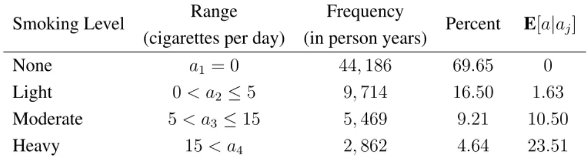
Table 1.2: Categorical Smoking Statistics

Smoking Level Range Frequency Percent E[a|aj]

(cigarettes per day) (in person years)

None a1 = 0 44,186 69.65 0

Light 0< a2 ≤5 9,714 16.50 1.63

Moderate 5< a3 ≤15 5,469 9.21 10.50

Heavy 15< a4 2,862 4.64 23.51

Table 1.2 reports the range of each of the intervals, the number of observations (in person years)

in each interval, and the mean of average cigarettes smoked per day conditional on being in the range

of the interval. The distribution of the average cigarettes smoked per day is skewed to the right with

the majority of the observations concentrated at the mass point of zero.

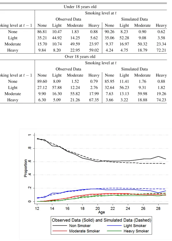
Table 1.3 reports the transition probabilities for the smoking categories. The transition

proba-bilities illustrate several key features of the data. First, individuals increase their level of smoking

(28)

Table 1.3: Cumulative Smoking Transition Probabilities

Smoking level att

Smoking level att−1 None Light Moderate Heavy

None 0.900 0.081 0.014 0.005

(36,748) (3,321) (562) (193)

Light 0.297 0.537 0.141 0.026

(2,679) (4,848) (1,269) (233)

Moderate 0.097 0.175 0.575 0.154

(482) (871) (2,862) (767)

Heavy 0.065 0.059 0.249 0.627

(169) (155) (650) (1,635)

Note: frequencies in parentheses

Table 1.4: Under 18 Smoking Transition Probabilities

Smoking level att

Smoking level att−1 None Light Moderate Heavy

None 0.882 0.099 0.015 0.004

Light 0.360 0.448 0.151 0.040

Moderate 0.116 0.146 0.517 0.221

(29)

several levels. Also, for any given level of smoking, there is a high probability that individuals will

transition to a lower level of smoking. For light and moderate levels of smoking, the probability that

individuals decrease the amount they smoke is approximately 30%. For the heaviest smokers, this

probability is almost 40%. The amount of decreases in the level of smoking observed in the data is

difficult to reconcile with the standard RA model, but is consistent with the model of behavior that

incorporates uncertainty and learning. Table 1.4 reports the transition probabilities for individuals

under 18 years old. Relative to the full sample there is less persistence in smoking choices, with

more movement (both upward and downward) between smoking categories. This is consistent with

the learning model since it will take some experience before individuals are able to determine what

level of smoking is optimal for their specific utility function parameters.

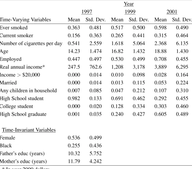
Table 1.5 presents summary statistics for smoking behavior and demographic variables in three

of the early waves.16 Over these waves, the proportion of individuals who currently smoke increases,

however, it does fall in later waves. The other variables included in the table enter the individual’s

decision to smoke, either directly through the utility received from smoking or through the cost of

smoking. The NLSY does not ask about parent’s smoking behavior. Parental smoking behavior

po-tentially enters the individual’s smoking decision through the individual’s beliefs as well as through

the cost of smoking. Parental education and other parental characteristics could serve as a proxy for

parent smoking behavior.

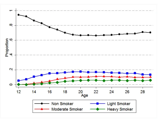
Figure 1.1 presents the proportion of individuals in each smoking category by age. The

propor-tion of individuals choosing to smoke increases steadily during the teenage years, reaches a peak for

individuals in their early 20s, and declines slightly as individuals progress through their 20s. The

decline in smoking rates for individuals in their 20s is primarily due to a lower proportion of light

smokers. The proportion of moderate and heavy smokers remains relatively constant after reaching a

peak around the age of 20. Figure 1.2 presents the proportion of current smokers by gender and race.

Blacks have a substantially lower rate of smoking compared to other ethnic groups, and females have

a lower smoking rate than males.

(30)

Table 1.5: Summary Statistics of Smoking and Demographic Variables in Select Years

Year

1997 1999 2001

Time-Varying Variables Mean Std. Dev. Mean Std. Dev. Mean Std. Dev.

Ever smoked 0.363 0.481 0.517 0.500 0.598 0.490

Current smoker 0.156 0.363 0.265 0.441 0.315 0.464

Number of cigarettes per day 0.541 2.559 1.618 5.064 2.368 6.135

Age 14.23 1.474 16.82 1.432 18.88 1.430

Employed 0.447 0.497 0.530 0.499 0.708 0.455

Real annual income* 247.5 762.6 1,208 3,178 3,889 6,295

Income>$20,000 0.000 0.014 0.010 0.098 0.028 0.164

Married 0.000 0.014 0.013 0.115 0.053 0.224

Any children in household 0.007 0.085 0.047 0.212 0.107 0.310

High School student 0.982 0.133 0.691 0.462 0.292 0.455

College student 0.000 0.020 0.128 0.334 0.303 0.460

High School graduate 0.001 0.035 0.240 0.427 0.605 0.489

Time-Invariant Variables

Female 0.536 0.499

Black 0.255 0.436

Father’s educ (years) 10.32 5.752

Mother’s educ (years) 11.79 4.242

(31)

Figure 1.1: Smoking Choice Probabilities by Age

(32)

1.4.3 Cigarette Prices and State Excise Tax Data

The cigarette tax and price data used in this paper are from Orzechowski and Walker’sTax Burden

on Tobacco. The price used is a sales weighted average of the premium brand cigarettes sold in a

given year. Cigarettes are taxed at the federal and state level. In some instances they are also taxed at

the county and municipal level. The federal cigarette tax in 2011 was $1.01 per pack. The tax rates

vary considerably across states. In 2011, state cigarette taxes ranged from a low of $0.17 per pack

in Missouri to a high of $4.24 in New York. At the start of the sample period in 1997, state cigarette

taxes ranged from a low of $0.025 in Virginia to a high of $0.825 in Washington. Historically,

the states with the lowest tax rates on tobacco are the tobacco-producing states of the southeast.

From 1997-2011, only two states have had a constant tax rate, and most states have had multiple

tax increases over the period. The variation in tax rates is largely responsible for the variation in the

retail price of cigarettes across states. In 2011, the average retail price of cigarettes per pack ranged

from $4.70 in Missouri to $10.29 in New York.

Table 1.6: Summary Statistics of State Tobacco Price and Taxes

Year Real Price Real Tax (State + Federal)

Mean SD Min Max Mean SD Min Max

1997 2.265 0.327 1.796 3.305 0.633 0.217 0.284 1.143

1998 2.477 0.353 2.013 3.576 0.661 0.256 0.280 1.310

1999 3.200 0.361 2.698 4.304 0.670 0.271 0.274 1.282

2000 3.318 0.393 2.777 4.512 0.760 0.279 0.365 1.450

2001 3.500 0.370 3.035 4.458 0.752 0.291 0.355 1.410

2002 3.787 0.550 3.107 5.671 0.927 0.432 0.397 1.819

2003 3.843 0.567 3.157 5.452 1.041 0.453 0.388 2.284

2004 3.815 0.615 3.088 5.343 1.064 0.515 0.378 2.598

2005 3.847 0.643 3.095 5.292 1.157 0.528 0.406 2.513

2006 3.772 0.673 2.899 5.365 1.135 0.527 0.393 2.533

2007 3.883 0.652 2.906 5.520 1.191 0.518 0.382 2.462

2008 3.896 0.737 2.893 5.687 1.244 0.579 0.368 2.511

2009 4.711 0.846 3.406 6.458 1.856 0.628 0.867 3.588

Table 1.6 present the summary statistics across the 50 states and the District of Columbia of the

(33)

over the sample period, and the amount of the average real tax increases by about three times. Over

the time frame, the variability in both the prices and taxes across states increases. Most years the

average real price increases due to increases in taxes. In years when there are no tax changes in a

state, the real price of cigarettes falls as the nominal price increases less than inflation.

Figure 1.3 shows how real retail cigarette prices and taxes have changed over time in New York

and North Carolina. Much of the price difference between these two states can be attributed to the

difference in their cigarette taxes. Also, the increase in the price of cigarettes over time is driven by

the increase in the tax rates. Other factors behind the increase in cigarette prices over this time period

are the Tobacco Master Settlement Agreement in 1998, and the increase in the federal cigarette

tax rate in 2009.17 Figure 1.4 shows the distribution of state cigarette tax rates over time. At the

beginning of the sample period, state cigarette taxes were relatively low. Over time, both the mean

and variance of the state cigarette tax distribution increased.

1.4.4 State Level Tobacco Policy Data

In addition to tobacco excise taxes, there are many other policies that states can pursue to

influ-ence the level of youth smoking. Some of these policies enter into the individual’s problem through

the budget constraint by imposing non-monetary costs on obtaining tobacco. Some examples of

policies that enter the individual’s problem in this way are restrictions on the sale of tobacco to

mi-nors, bans on the sale of tobacco in vending machines, and restrictions on free samples of tobacco

products. Another way for tobacco policies to influence behavior is through restrictions on tobacco

consumption. The overall utility one receives from smoking will be less if there are restrictions on

where and when one can smoke. Examples of restrictions on tobacco consumption are indoor

smok-ing bans and smoke-free schools. Finally, some tobacco policies influence the individual’s beliefs

and expectations. In the context of this paper, these policies influence the individual’s initial prior

beliefs. Examples include restrictions on cigarette advertisements, funding of tobacco prevention

17_{In 1998, 46 states came to an agreement with the four largest cigarette manufacturers. The states agreed to drop their}

(34)

Figure 1.3: Real Cigarette Taxes and Prices in NY and NC (in year 2000 dollars)

(35)

and education programs, and requiring tobacco education in schools. The data on state tobacco

poli-cies are from the Centers for Disease Control (CDC), the National Cancer Institute (NCI), and the

Substance Abuse and Mental Health Services Administration (SAMHSA).

1.5 Estimation

1.5.1 Likelihood Function

Define the conditional value function for alternativej as the deterministic portion of flow utility from that alternative (i.e., utility minus the preference shock) plus the discounted expected future

value of lifetime utility conditional on alternativej being chosen. Then, the conditional value func-tion associated with alternativejin periodtis given by:

vj_nt(Snt,Γnt, Xnt) = αn+Et[ρn|Γnt]g(Snt) +ξjXntz(aj)−Et[τn|Γnt]Snt1[aj >0]

−Et[ωn|Γnt]q(aj, Snt)1[aj < Snt]−γnptaj+βEt[Vn,t+1(Sn,t+1,Γn,t+1, Xn,t+1)|djnt = 1] (1.13)

where

Vn,t+1(Sn,t+1,Γn,t+1, Xn,t+1) = E[max

j v j

n,t+1(Sn,t+1,Γn,t+1, Xn,t+1) +jn,t+1] (1.14)

The expectation over the future value term is taken with respect to the distribution of future beliefs,

future demographic state variables, and future prices. The evaluation of current period utility depends

upon the mean of the prior beliefs only. The variance of the prior does affect the expectation over

future beliefs. The utility from not smoking is normalized to include the cost of withdrawal only,

so ξ1 = 0. The state variables are the level of smoking stock (i.e., last period’s smoking decision)

and the individual’s beliefs, denoted by Γ, which include beliefs about parameter values and future prices.18 _{I assume an i.i.d. type I extreme value (EV) preference shock.}19 _{The choice probabilities}

18_{The price process has yet to be formally incorporated into the model, so the following estimation routine assumes}

perfect knowledge of future prices. The proposed estimation routine can be extended to estimate the parameters of a random price process.

19_{One of the major limitations of the multinomial logit model is the assumption that the shocks are uncorrelated over}

(36)

after experimentation are given by:

P_ntj = e vntj

PJ k=1ev

k nt

forj = 1, . . . , J (1.15)

For individuals who have never smoked, they first choose whether or not to experiment, and then,

conditional on experimenting, they decide the level of smoking. LetdE_nt be an indicator variable that equals one if the individual experiments in periodt. The conditional value of experimenting is:

vE_nt = (E[αn|Γnt] +ξEXnt)z(aE)−γptaE+Et[Vnt|dEnt = 1] (1.16)

The conditional value function of not experimenting is simply the discounted expected maximum

of the next period’s value function conditional on not experimenting and not consuming any of the

addictive good. The probability for experimenting, PE

nt, is given by the Logistic cumulative

distri-bution function. For an individual who has never smoked prior to period t, the behavior in periodt

is captured by the joint probability of experimenting and level of smoking (PE ntP

j

nt). The decision to

experiment is made based on the individual’s belief about his level ofα, soPE

ntis calculated based on

an individual’s beliefs. If he decides to experiment, he learns his true level ofα, soP_ntj is calculated using the individual’s true value ofα.

There are a total ofN individuals, and each individual is observed for a total ofT + 1periods. The likelihood of individualnmaking the sequence of choices{∪j{djnt}, dEnt}Tt=1is:

Ln

γ, ξ |θn,Γn,0,Λn = T Y t=0 _YJ j=1

Pj d

j nt

nt Ant

∗

(1−P_ntE)1−dEnt _PE

nt J Y

j=1

Pj d

j nt

nt

dEnt1−Ant

(1.17)

whereAnt is an indicator for the individual having ever smoked prior to periodt. If the individual

has smoked prior to period t (i.e., Ant = 1), the individual makes a consumption decision. If the

individual has not smoked prior to period t (i.e., Ant = 0), then the individual makes a sequential

(37)

experimentation and consumption decision. This individual likelihood is conditional on the

individ-ual’s true addictive parameters (θn), the distribution of individual’s initial prior beliefs (Γn,0), and a

given sequence of signal noise draws (Λn = {ψnt, λnt, ηnt}Tt=0). This formulation is equivalent to

conditioning on the individual’s beliefs at timetsince the beliefs in timetare completely determined by the individual’s initial prior, the sequence of signal noise, and the sequence of choices. Since the

individual’s true parameters and signal noise sequences are not observed by the researcher, the

un-conditional likelihood is calculated by integrating the un-conditional likelihood over the distribution of

these unobserved variables:

Ln(γ, ξ, σ2ψ, σλ2, ση2,θ,¯ Σ) = Z

θ Z

Λ

Ln

γ, ξ|θn, mn,0,Σn,0,Λn

dF(Λ|σ_ψ2, σ_λ2, σ_η2)dF(θ|θ,¯ Σ) (1.18)

and the full log-likelihood function is given by:

L(γ, ξ, σ2_ψ, σ_λ2, σ_η2,θ,¯ Σ) =X n

logLn(γ, ξ, σ2ψ, σ

2

λ, σ

2

η,θ,¯ Σ)

(1.19)

The total dimensions of unobserved variables is3∗T + 4.20 The integrals do not have a closed form solution, so they must be approximated numerically. The parameters to be estimated include the

util-ity function parameters (γ, ξ), the mean and covariance matrix of the population distribution of the rational addiction parameters(¯θ,Σ), and the variances of the signal noise distributions(σ2

ψ, σ2λ, σ2η).

1.5.2 Identification

The model parameters are identified through the observed sequences of smoking decisions. The

parametersξandγare identified through differences in smoking decisions between individuals with different observable characteristics. The price sensitivity parameter γ is identified by both cross-sectional variation and variation over time in the price of cigarettes. The utility from not smoking

when the smoking stock is zero is normalized to zero. The parameter α affects the utility for each

20_{The dimension of the unobserved signals is likely to be less than 3*T since some of the signals are observed by}

(38)

level of smoking regardless of past smoking. The reinforcement parameter captures the effect of the

interaction between the current level of smoking and the smoking stock. The tolerance parameter

only depends on the smoking stock, so, for a given level of smoking stock, a change in the tolerance

parameter only affects the probability of smoking versus not smoking. The reinforcement parameter

affects the probability of smoking versus not smoking, but it also affects the probability of each

level of smoking. The withdrawal parameter only affects the utility of a reduction in the level of

smoking from one period to the next, so this parameter is identified by smokers who reduce their

level of smoking or quit smoking entirely. The match, tolerance, reinforcement, withdrawal, and

price sensitivity parameters do not vary across alternatives. Differences in utility for the different

levels of smoking for these parameters are ultimately a result of the functional form assumptions.

The individual-specific parameters are not point identified for each individual. There is no way

to estimate a specific value of these parameters for each individual. Also, since these parameters

are continuous, a distributional assumption is required for the population distribution of parameters.

Then, given that the conditional value function is defined over the support of the distribution of the

unobserved continuous variables, the parameters of the population distribution (mean and

covari-ance) are identified. The identification behind the learning process is driven by the fact that the

valuation an individual attributes to each alternative depends upon the individual’s current beliefs

only and not the individual’s true parameters. The individual’s beliefs converge to the true

param-eters as the individual receives additional signals. Therefore, individuals with a lot of experience

will behave according to their true parameter values. Also, if an individual knows his true parameter

values, he can use the model to calculate an optimal consumption sequence. Differences between the

optimal consumption sequence if the individual knows his true parameter values and the decisions of

the individual when he is inexperienced are driven by the difference between the individual’s beliefs

and his true parameter values. The speed at which the individual’s consumption sequence converges

to the optimal consumption sequence with full knowledge identifies the speed of learning (i.e., the

variance of the signals). Additional restrictions on the learning process are necessary for

identifi-cation. These include restrictions on the initial prior beliefs (Rational Expectations), distributional

(39)

1.5.3 Estimation Procedure

There are several computational requirements that make estimation of the parameters of the

model by Full Information Maximum Likelihood difficult. The main issue is that the evaluation of

the log likelihood function requires integrating over the continuous distribution of population

param-eters and over all possible sequences of signal noise. Simulated maximum likelihood is one method

that is used to overcome this problem. The unconditional likelihood function is approximated

nu-merically by taking random draws from the distribution of the unobserved variable, evaluating the

conditional likelihood, and taking the average of the conditional likelihoods over the draws.

Evaluat-ing the conditional likelihood, however, for a sEvaluat-ingle draw still involves significant computation. The

solution to the individual’s problem requires integrating over future beliefs, which are

multidimen-sional continuous variables. One way to reduce the computational burden of evaluating the value

function is to use the Conditional Choice Probability (CCP) method of Hotz and Miller (1993).

Hotz and Miller (1993) show that when the preference shock has a GEV distribution, the future

value term in the conditional value function can be expressed as a function of future flow utilities

and conditional choice probabilities (CCPs). For certain classes of problems (e.g., optimal stopping

problems), taking the difference in conditional value functions leads to the future value term only

containing one period ahead flow utilities and CCPs. In other problems, the future value term

asso-ciated with the difference in conditional value functions contains flow utilities and CCPs for a finite

number of future periods. This property is called finite dependence, and it is a feature of the

prob-lem in this paper.21 Standard CCP estimation involves estimating the CCPs in a first stage using the

data and using the estimated CCPs to calculate the individual’s value function. One limitation of the

standard method is that it do not allow for unobserved heterogeneity. Arcidiacono and Miller (2011)

develop a method of CCP estimation that allows for a finite distribution of unobserved

heterogene-ity by using the Expectation Maximization (EM) algorithm. The unobserved heterogeneheterogene-ity in this

paper are the individual’s beliefs and the individual’s true parameter values, which are both

continu-ous. James and Matsumoto (2013) extend the work of Arcidiacono and Miller (2011) to allow for a

(40)

continuous distribution of unobserved heterogeneity.

It can be shown that the values of the parameters that maximize the likelihood function (1.19)

also maximize the following transformed likelihood function:22

L(γ, ξ, σ_ψ2, σ2_λ, σ2_η,θ,¯ Σ) =X n

Z

θ Z

Λ

πn(θn,Λn)

X

t (1−Ant)

(1−dE_nt)log(1−P_ntE) +dE_ntlog(P_ntE)+X j

dj_ntlog(P_ntj)

dΛdθ (1.20)

whereπis the conditional probability that the parameter values are θ, θ0, andΛgiven the observed

choices. This conditional probability is given by:

πn(θn,Λn) =

f(θn|θ,¯ Σ)f(Λn|σψ2, σ

2

λ, σ

2

η) Q

tLnt(θn,Λn) R

θ R

Λ

Q

tLnt(θn,Λn)f(Λn|σψ2, σ2λ, σ2η)f(θn|θ,¯ Σ)dΛdθ

(1.21)

The estimation routine in this paper used the likelihood function in equation 1.20. The procedure

starts by taking M draws from the distribution of the unobserved variables for each individual as well as initial guesses for the values of the parameters and the CCPs. The estimation proceeds by

using the EM algorithm, specifically a simulated EM algorithm (SEM). The EM algorithm is an

iter-ative procedure that alternates between an expectation step (or E-step) and a maximization step (or

M-step). The E-step updates the CCPs and π using the prior iteration values of the parameters and CCPs. The M-step updates the value of the parameters by maximizing the likelihood function using

the updated CCPs andπ. The estimation continues to iterate over these two steps until the parameter estimates converge. The use of the EM algorithm to incorporate unobserved heterogeneity has

sev-eral advantages.23 _{The most significant advantage is that the EM algorithm, or the SEM algorithm}

in the current context, reintroduces additive separability of the likelihood function. This property

allows for sequential estimation of the likelihood function. In the current context, additive

separa-bility of the likelihood function allows for the parameters of the experimentation and consumption

22_{This is the expected conditional (on the unobserved variables) likelihood, where the expectation is taken with respect}

to the distribution of the unobserved variables conditional on the observed variables and the choices.

(41)

decisions to be estimated separately. The estimation procedure is presented in greater detail in the

Estimation Appendix.

1.5.4 Initial Conditions

The first period that individuals are observed in the NLSY97 is not the same as the initial period

of the individual’s optimization problem. That is, individuals may enter the estimation sample having

already smoked. The values of the state variables in the initial wave of data depend on prior decisions

and state variables that are not observed by the researcher. Some individuals have never smoked by

the first wave. Others have smoked at some point prior to the first wave but are not observed to

smoke in the first wave. Finally, some individuals are regular smokers at the first wave. The latter

two groups present an initial conditions problem both in that the prior year’s smoking is not observed

in the first period and it is not observed how much they have learned. Individual’s initial prior beliefs

also present an initial conditions problem. I assume that individual initial priors are identical to the

population distribution of the parameters (i.e., Rational Expectations).24

For individuals who have smoked prior to the first wave, the amount smoked in the period prior to

the first wave is treated as discrete unobserved heterogeneity. The individual likelihood is calculated

for each possible alternative in periodt = 0. The probability that the individual selected alternative

j in periodt= 0is:

P_n,j₀ = 1

1 +exp(ξ_ICj XIC n,0)

(1.22)

The individual likelihood is calculated by multiplying the likelihood conditional on selecting

alter-nativej in periodt = 0by the probabilityP_n,j₀ and summing over the alternatives. 1.5.5 Functional Forms

The utility for the smoking level associated with alternativej, contains several modifying func-tions. The purpose of these functions is to allow for utility to be nonlinear in both the level of

smoking and the level of past smoking. In order to estimate the parameters of the model, these

generic functions must be replaced with specific functional forms. The function z(a)incorporates

24_{In future work, I will attempt to parameterize the initial priors by allowing the mean of the initial priors (and perhaps}