Assessing the Impact of the Urban Tree Canopy on Streamflow Response: An Extension of Physically Based Hydrologic Modeling to the Suburban Landscape
Tamara Shira Mittman
A thesis submitted to the faculty of the University of North Carolina at Chapel Hill in partial fulfillment of the requirements for the degree of Master of Arts in the Department of Geography
Chapel Hill 2009
ii
ABSTRACT
TAMARA MITTMAN: Assessing the Impact of the Urban Tree Canopy on Streamflow Response: An Extension of Physically Based Hydrologic Modeling to the Suburban
Landscape
(Under the direction of Lawrence E. Band)
TABLE OF CONTENTS
List of Tables ... vi
List of Figures ... vii
1. Introduction ... 1
2. Background ... 3
a. Significance ... 3
b. Review of empirical studies of urbanization impacts on hydrology... 7
c. Review of modeling studies of urbanization impacts on hydrology ... 11
d. Model calibration in ungauged catchments ... 15
e. Model validation for studies of land cover change ... 16
f. Model uncertainty ... 17
3. Statement of Problem ... 19
4. Study Area Description ... 21
a. Topography ... 21
b. Soils... 21
c. Vegetation and Land Cover ... 22
d. Climate and Precipitation ... 22
5. The Regional Hydro-Ecological Simulation System (RHESSys)... 24
a. Interception ... 24
iv
c. Vegetation Growth ... 26
d. Infiltration ... 26
e. Surface and subsurface flows ... 27
f. Deep groundwater flows ... 29
6. Datasets ... 30
a. Climate time series ... 30
b. GIS datasets ... 31
c. Default files ... 31
d. Streamflow time series ... 32
7. Methods ... 35
a. Spatial Data Processing ... 35
i. Catchment Delineation ... 35
ii. Catchment Topography and Soils ... 36
iii. Catchment Land Use and Land Cover Layers ... 37
iv. Catchment Flowpaths... 38
b. Calibration and Validation ... 39
c. Simulation of Vegetation Management Practices ... 42
8. Calibration and Validation Results ... 44
a. Calibration ... 44
b. Validation... 45
9. Vegetation Management Results ... 48
a. Impact of Vegetation Management on Streamflow Regime ... 48
c. Impact of Vegetation Management on Evapotranspiration ... 51
d. Impact of Vegetation Management on Soil Moisture ... 53
10. Discussion... 56
a. Research Questions ... 56
b. Model and methodology shortcomings ... 64
11. Conclusion ... 66
a. Implications for land use planning ... 66
b. Future research ... 67
Appendix A: Tables ... 70
Appendix B: Figures ... 76
vi
LIST OF TABLES
Table
LIST OF FIGURES
Figure
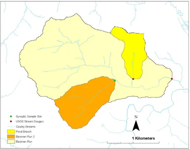
4. 1: Location of study catchments. ... 76
4. 2: DEM of study catchments... 77
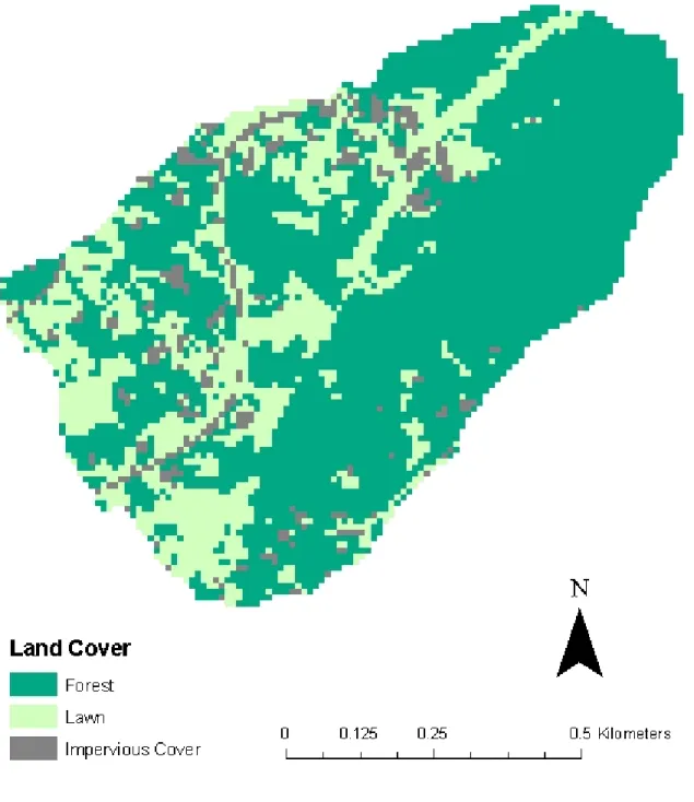
4. 3: Land cover classification for BR3. ... 78
4. 4: Location of stream gauges and synoptic sample sites. ... 79
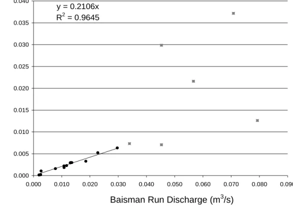
4. 5: Regression of synoptic samples against streamflow from BR. ... 80
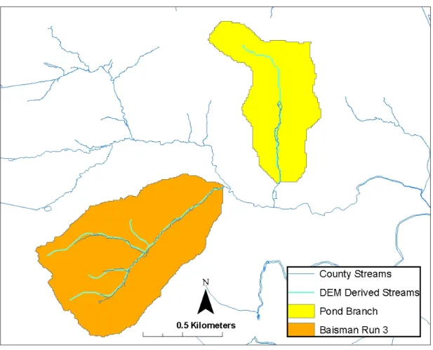
4. 6: Catchment boundaries and stream network ... 81
4. 7: Hillslope boundaries. ... 82
4. 8: Estimated soil distribution in BR3. ... 83
4. 9: Location of areas converted from lawn to forest. ... 84
5. 1: Pond Branch model performance for LAI of 5. ... 85
5. 2: Validation results for calibrated parameter sets. ... 86
5. 3: Prior and posterior distributions of significant parameters. ... 87
5. 4a: Pond Branch model performance: Daily scale. ... 88
5. 4b: Pond Branch model performance: Monthly scale. ... 88
5. 4c: Pond Branch model performance: Annual scale. ... 82
5. 5a: Baisman Run 3 model performance: Daily scale. ... 91
5. 5b: Baisman Run 3 model performance: Monthly scale. ... 91
5. 5c: Baisman Run 3 model performance: Annual scale. ... 91
5. 6: Daily model bias. ... 94
5. 7: Management impact on Q: Annual scale. ... 95
5. 8: Management impact on Q: Daily scale. ... 96
viii
5. 9b: Seasonal distribution of rainfall. ... 90
5. 10: Management impact on Q: Conversion of upslope vs downslope lawn. .... 99
5. 11: Sensitivity of management impact to grass root depth: Actual and entirely forested scenarios ... 100
5. 12: Sensitivity of management impact to grass root depth: Forested upslope and forested downslope scenarios. ... 101
5. 13: Management impact on ET: Annual scale. ... 102
5. 14: Management impact on ET: Monthly scale. ... 103
5. 15: Comparison of management impact on E and T. ... 104
5. 16: Spatially distributed change in annual ET. ... 105
5. 17: Management impact on saturation deficit: Daily scale. ... 106
5. 18: Management impact on saturation deficit: Conversion of upslope vs downslope lawn. ... 107
5. 19: Spatially distributed saturation deficit after a summer storm. ... 108
5. 20: Spatially distributed saturation deficit after a winter storm. ... 109
1.
Introduction
This thesis examines the impact of land cover composition and pattern on urban hydrologic response. Though planning practice assumes a relationship between urban pattern and aquatic ecosystem function, scientific knowledge of this relationship is limited (Alberti, 2005). Extensive research has documented the impacts of land cover composition on hydrologic response and examined the mechanisms through which these impacts are generated, but the interaction of these mechanisms with land cover pattern remains poorly understood. To advance our understanding of hydrologic processes and pathways in the urban environment, this study explores the hydrologic response of a suburban catchment in Baltimore, Maryland to different patterns of vegetation. We integrate field data collected by the Baltimore Ecosystem Study, part of the Long Term Ecological Research (LTER) network established by the National Science Foundation, with a distributed ecohydrologic simulation system to develop models of the study catchment and a nearby reference catchment.
2
2.
Background
a.
Significance
Research has demonstrated that urban development dramatically alters catchment hydrologic response. Urban development alters the hydrologic cycle by armoring the landscape with pavement and rooftops and altering soils and vegetation (Walsh 2005a, Walsh 2005b, Endreny 2005, Riley 1998). These changes reduce infiltration and
evapotranspiration and increase runoff volumes. Urban drainage systems amplify these changes by conveying all runoff to the nearest water body, producing flashy flow regimes with high peak flows.
4
the runoff rate and not the runoff volume, they cannot prevent stream channel erosion and the associated economic and ecological impacts (Booth and Jackson 1997, Emerson 2005, Endreny 2005, Walsh 2005b).
As the urbanization of the American landscape continues, damage to aquatic ecosystems will likely follow. According to the USDA’s Natural Resource Inventory, the area of developed land in the United States (defined as “large urban and built-up areas, small built-up areas, and rural transportation land”) increased by ~48% between 1982 and 2003 – an area approximately equal to that of the state of New York. Most of this
development occurred on land that was previously forested or farmed, and much of it created new suburbs (Alig 2004, Brown 2005, Theobald 2005). The pace at which we are transforming the landscape exceeds the rate of population growth. Whereas the area of urban, suburban, or exurban land uses increased by an average of 1.6% per year between 1980 and 2000, the population increased by an average of only 1.18% per year (Theobald 2005).
instance, states as its goals the reduction of local flooding, the reduction of stream channel erosion, the maintenance of predevelopment hydrology (including groundwater recharge and baseflows), the reduction of pollution, and the reduction of siltation and sedimentation. To achieve stormwater management goals, state legislation generally includes an associated set of standards informed by science. Because research has suggested that a large proportion of stream channel erosion occurs at an “effective discharge” approximately equal to the bankfull flow, most state legislation requires the control of runoff rates to maintain the frequency of a design flow (Doyle et al. 2002). Because more recent research has suggested that frequent, smaller events may be more important causes of channel incision than infrequent, larger events, recent legislation often requires the control of runoff volumes as well as rates (Walsh 2005b). Other stormwater standards vary significantly from state to state, but often include constraints on pollutant loads and annual recharge volumes.
A gradual transition in the principles and practice of stormwater management has accompanied the changes in state and federal standards. Whereas stormwater
management was once the domain of engineers who developed centralized, “end-of-the-pipe” facilities to control property damage from large infrequent storms, in recent years the objectives of stormwater management have evolved to address a more diverse set of impacts across a broader range of spatial and temporal scales (British Columbia Ministry of Water, Land, and Air Protection, 2002). In the United States, many planning
6
addressing impacts at the regional and catchment scales as well as the site scale, and by addressing flow regimes as well as peak flows. To address impacts at larger spatial scales, LID identifies and preserves sensitive areas, confining all development to a
“development envelop” (Prince George’s County, 2000). Sensitive areas include variable source areas, riparian areas, wetlands, areas with steep slopes, and areas with high
permeability soils. To mimic predevelopment hydrology across a range of precipitation events and soil moisture conditions, LID applies distributed as well as centralized practices that increase infiltration and evapotranspiration as well as storage. These practices include the minimization of impervious cover, the management of urban vegetation, and the installation of “soft-engineering” facilities such as rain gardens, grassed swales, and green roofs.
Though science and policy have converged on the objective of mitigating the hydrologic impact of urban development, scientific knowledge at the scale and resolution demanded by urban planning remains poorly developed. Planners operate across large scales, developing plans for entire towns, cities and counties. While much research has examined the impacts of development at the catchment scale, research on the
(vegetation management) to begin to provide insight into the mechanisms through which urban pattern affects catchment hydrologic response.
b.
Review of empirical studies of urbanization impacts on hydrology
An extensive review of the literature indicated that empirical studies of the impact of land cover change on urban hydrologic response generally examine land cover
composition, rather than land cover pattern, and the significance of impervious cover, rather than the significance of vegetation type. Decades of empirical research have documented relationships between the extent of impervious cover within catchments and various measures of stream health. Studies have noted dramatic changes in flow regime (Konrad 2001, Burns 2005, Chang 2007, Changnon 1996, Dow 2007, Jennings 2002, Rose 2001), channel geomorphology (Hammer 1972, Doll et al 2002), pollutant loading and timing (Griffin 1980, Shields 2006, 2008), habitat quality (Cianfrani 2006), and biological assemblages (Klein 1979, Moore and Palmer 2005, Morley 2002, Strayer 2003, Snyder 2003) as impervious cover within catchments increases. Though earlier research noted a minimum threshold below which ecosystem degradation was negligible (Booth and Jackson 1997, Arnold and Gibbons 1996, Klein 1979), more recent research attributes this threshold to measurement imprecision and demonstrates a continuous decline in measures of biological integrity as % imperviousness exceeds zero (Walsh et al 2005a, Booth et al. 2004, Booth et al 2002, Moore and Palmer 2005, Karr and Chu 2000, May and Horner 2000, Booth et al., 2001).
8
While several empirical studies have documented improvements in stream health as percent forest cover within urbanized catchments increases, we found no studies examining the impact of vegetation type on catchment hydrologic response. In his classic analysis of the relationships between stream channel enlargement and land cover in urbanized watersheds, Hammer found land in forest to have a negative relationship to channel enlargement (1972). Research relating forest and impervious cover to measures of stream biotic integrity has consistently demonstrated that both land covers are
important predictors of stream health, observing measures of biotic integrity to increase with forest cover and decrease with impervious cover (Goetz and Fiske 2008, Carlisle and Meador 2007, Strayer 2003, Steedman 1988). In his study of 10 catchments in southern Ontario, Steedman not only found basin Index of Biotic Integrity (IBI) scores to be directly related to forest cover and inversely related to urban land cover, but noted a greater impact on biotic integrity per increment change in forest cover. It is hoped that the present study will elaborate upon this research to provide insight into the role of urban grasses as well as trees in shaping catchment hydrologic response.
Previous research indicates that the mechanisms through which changes in land cover degrade stream health are largely driven by changes in catchment hydrology. Removal of upland and riparian vegetation and addition of impervious cover and drainage systems transform land-water linkages, reducing interception,
ultimately, reduced biologic integrity (Moore Palmer 2005, Allan 2004, Snyder 2003). Again while several empirical studies have addressed the impact of urban forests on catchment hydrologic processes, none have explicitly addressed the relative impact of different types of vegetation.
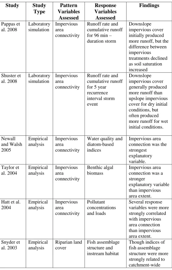
In recent years, interest has increased in the impact of land cover pattern, as well as extent, on hydrologic and ecosystem response (Alberti 2005, King 2005). Recent research into the effects of urbanization on aquatic ecosystem function has examined several components of landscape pattern, including: 1) the connectivity of impervious cover to stream channels, 2) the composition of land cover within the riparian corridor, 3) the distance of land covers from the stream channel, and 4) the size of land cover patches. The most extensively studied components to date are the connectivity of impervious cover and the composition of riparian land cover. Empirical studies of the relationships between catchment physical characteristics and various measures of
ecosystem function have consistently found that ecosystem function is better predicted by the extent of connected impervious cover than by the extent of all impervious cover (Newall and Walsh 2005, Taylor et al 2004, Hatt et al 2004, Hammer 1972). Laboratory simulations of rainfall on various arrangements of pervious and impervious surfaces have also shown impervious connectivity to have a significant impact on runoff volume
10
through which spatial arrangement shapes the impact of land cover change remains limited.
Extensive scientific research has also accumulated on the impact of riparian forests on ecosystem function. In constructing empirical models of stream biotic integrity, many researchers have examined the relative predictive power of catchment-wide versus riparian land covers. Their conclusions are inconsistent. Several authors have found that riparian land cover is a significant predictor of in-stream habitat but not fish biological assemblages, suggesting that alterations in flow regime and reductions in water quality overwhelm the capacity of riparian vegetation to maintain biological integrity (Snyder 2003, Strayer 2003). In contrast, other authors have found that riparian forests protect invertebrate diversity even in catchments with substantial urbanization (Carlisle and Meador 2007, Moore and Palmer 2005, Steedman 1988).
Research has only recently become available on the impact of landscape position and land cover aggregation on aquatic ecosystem function. Perhaps the earliest study to assess the impact of landscape position was Hammer’s classic analysis of channel
empirical models have stated their conclusions in less certain terms. Both King (2005) and Goetz and Fiske (2008) included distance-weighted variables in their assessments of land cover variables as predictors of stream biotic integrity. King et al found that weighting of developed land by distance from the sampling station provided better predictions of biotic integrity than land cover percentages alone. Goetz and Fiske found that weighting of land covers by distance from the stream increased model performance, but noted that the distance weighting scheme that was most effective integrated tree cover density and distance from the stream. Alberti et al (2007) applied landscape ecology metrics to examine the impact of land cover pattern on stream biotic integrity. Their research found that mean patch size of impervious areas and mean patch size of forested areas explained much of the variability in stream biotic integrity, but were so highly correlated with the amount of impervious area that no conclusions could be drawn. Some empirical studies have found that the explanatory power of land cover composition variables declines in smaller catchments, suggesting that the spatial arrangement of land covers becomes more important at smaller scales (King 2005, Strayer 2003). Whereas significant research has examined the mechanisms through which the connectivity of impervious cover and the composition of riparian land cover impact stream health, little is known about the mechanisms through which landscape position of different land covers impact stream health.
c.
Review of modeling studies of urbanization impacts on hydrology
12
impacts of future urban development on hydrologic response, and 2) providing insight into the mechanisms through which development impacts hydrologic response. In the first case, empirical research is difficult if not impossible because measurements (either of the pre-developed past or developed future) are often unavailable, while in the second case empirical research is possible, but so many measurements would be required to properly account for spatial and temporal heterogeneity in catchment characteristics and climate variables that empirical research becomes prohibitively costly and complex (Cuo et al 2008).
The structure of the hydrologic models most commonly applied to the
simulation of urban catchments has confined most research to the analysis of land cover composition (rather than pattern) and impervious land cover (rather than vegetation). Refsgaard (1996) identified three model structures commonly applied in hydrologic simulation: 1) empirical black box, 2) lumped conceptual, and 3) distributed physically based. The vast majority of the modeling systems applied to the simulation of land cover change in urban catchments belongs to the second class. Lumped conceptual models partition catchments into hydrologically similar areas and attempt to represent hydrological processes by calculating fluxes of water and mass to and from these areas. Though the entire constellation of urban hydrologic models characterized by this
(McColl 2007, Girling and Kellet 2002, Bhaduri 2000, Choi 2003, Miller 2002, Tang 2005, Wu 2007). These models generally partition a catchment into areas with similar land covers, assign a set of soil moisture-dependent curve numbers to each land cover, and apply the SCS equation to each land cover to estimate overland flow at each time step. Among the many shortcomings associated with this approach (see Garen and Moore, 2005) is the difficulty of assigning any physical meaning to the empirically-derived “curve numbers” (Beven 1989). Because the curve number lacks physical meaning, it is difficult to select a curve number that reflects patterns of land cover or vegetation processes.
Another model commonly applied to the prediction of the hydrologic impacts of urbanization is the federally-supported HSPF simulation system (Booth et al 2002, Brun and Band 2000). Though HSPF is more process-based than curve number
models, its structure still cannot support analysis of the impact of land cover patterns or vegetation processes. In HSPF, segments (or sub-catchments) may be assigned
pervious and impervious percentages, but the model cannot account for the arrangement of pervious and impervious areas within sub-catchments and their interaction (such as the re-infiltration of run-off, for example). One study has attempted to analyze the impact of urban vegetation in HSPF, finding that the
conversion of forest to lawn was more significant than impervious cover in determining peak discharge increases from exurban catchments (Booth et al 2002). Other
14
evapotranspiration processes in HSPF is too crude to support the analysis of vegetation effects (Wang et al 2008).
While empirical research on urbanized catchments suggests that both land cover composition and land cover pattern are significant determinants of aquatic ecosystem function, it has not identified the mechanisms through which urban pattern shapes urban hydrologic process. Lumped conceptual models of urban catchments have also provided little insight into the role of urban pattern. Research suggests, however, that distributed physically based models of urbanized catchments have great potential to advance our understanding of the effects of land cover pattern on hydrologic response. The following sections discuss three obstacles that limit the use of hydrologic
simulation models to assess the impacts of land cover change in urban catchments.
d.
Model calibration in ungauged catchments
16
range of plausible parameter values (Tague and Pohl-Costello, 2008). Model findings can then be assessed in the context of the sensitivity of the results to model parameters. A third approach is to collect a limited number of streamflow measurements to calibrate the catchment model. Studies conducted as part of the Prediction in Ungauged Basins initiative (PUB) indicate that as few as 6 measurements can be effective in constraining prediction uncertainties (Seibert and Beven 2009).
e.
Model validation for studies of land cover change
available before and after land cover change occurs, this test is often impossible to implement. Ewen et al (1996) suggested that another appropriate test for a model intended to predict the effects of land cover change is the proxy-catchment test. Proxy-catchment tests involve calibration of a model for one Proxy-catchment, adjustment of model parameters to reflect a second catchment, and validation of the model for the second catchment.
f.
Model uncertainty
All model predictions are limited by uncertainty derived from many sources including: model structural error, errors in model input data, errors in output-variable measurements, uncertainty in parameter values, and uncertainty in initial conditions. One technique for quantifying model predictive uncertainty frequently employed in
environmental simulation modeling is the generalized likelihood uncertainty estimation methodology (GLUE) developed by Beven and Binley (1992). In the GLUE
methodology, parameters sets are randomly sampled from a prior distribution of
parameter values (often a uniform distribution) and used to run the model. Model output for each parameter set is assessed using a likelihood measure (sometimes called a
18
questioned the ability of the GLUE methodology to address model uncertainty derived from model errors, input-data errors, or output-variable measurement errors (Stedinger et al, 2008). Even this criticism, however, concedes that the GLUE methodology provides insight into model sensitivity to parameter values. Though the GLUE methodology is now widely recognized to be a subjective technique that generates qualitative uncertainty bounds, it is also widely applied as a simple approach to uncertainty estimation in
3.
Statement of Problem
Though much research has examined the impacts of urban and suburban
development on water resources, and though many planners and policy makers are eager to mitigate these impacts, scientific knowledge that might advance policy or practice is lacking (Alberti et al 2007, Wolosoff and Endreny 2002).
One approach to mitigation that has attracted great interest is the management of vegetation in urban and suburban areas to increase interception, evapotranspiration, and infiltration. Though some research has addressed the impact of expanded tree canopies on hydrologic response, none has addressed the impact of the spatial distribution of vegetation.
Distributed, physically-based hydrologic models offer significant advantages over empirical and lumped-conceptual models in understanding the effects of land cover change on catchment hydrologic response (Beven 2001). To date, however, few studies have applied such models to urban catchments.
20
response. This thesis focuses on the impact of vegetation patterns. The themes and questions addressed by this study are presented below:
Theme A: Application of a distributed, physically based model to an ungauged urban catchment
• Question A1: Can calibrated soil and groundwater parameters from a
forested reference catchment be transferred to an ungauged suburban catchment?
• Question A2: Can a distributed, physically based model accurately
reproduce streamflow from a suburban catchment?
Theme B: Prediction of the impact of land cover composition and pattern on catchment hydrologic response.
• Question B1: What is the impact of different extents of tree cover in a
suburban catchment on aggregate catchment response? Does this impact exceed the uncertainty generated by parameter uncertainty?
• Question B2: What is the impact of different patterns of tree cover in a
suburban catchment on aggregate catchment response? Does this impact exceed the uncertainty generated by parameter uncertainty?
• Question B3: What is the impact of different patterns of tree cover in a
4.
Study Area Description
a.
Topography
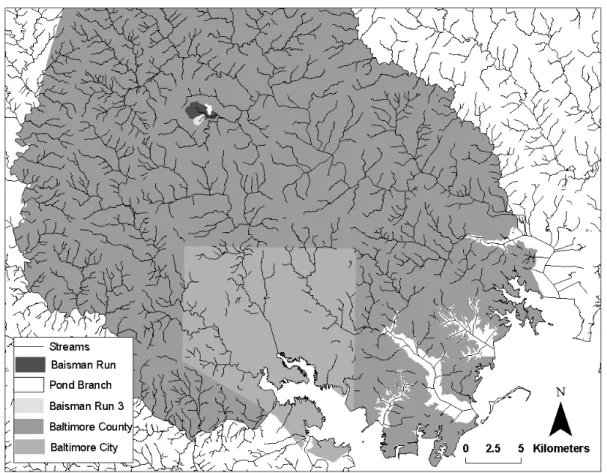
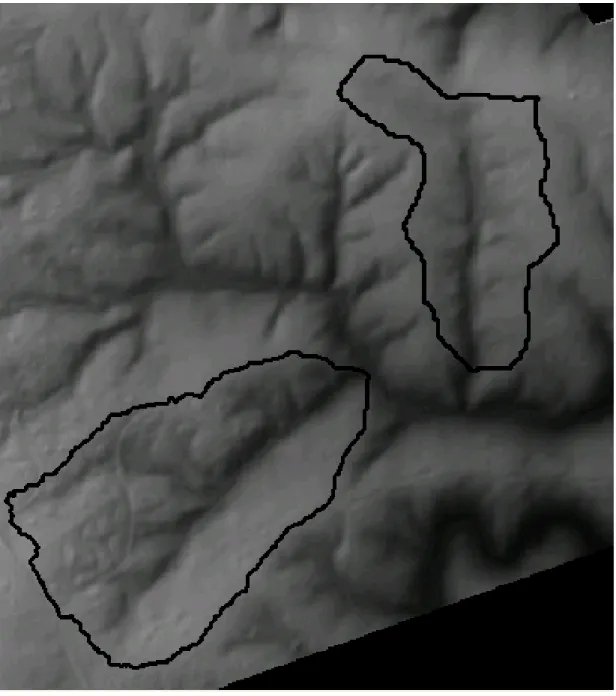
Pond Branch (PB) and Baisman Run 3 (BR3) are sub-catchments of the
extensively studied Baisman Run catchment in the Piedmont region of Maryland (Figure 4.1). Pond Branch is a 0.31 km2 catchment with elevations ranging from 190 m along the northwestern crest to 130 m at the outlet to the south (Figure 4.2). Gentle upland slopes and steep side slopes drain to a broad riparian area containing a perennial headwater stream. The stream channel is relatively narrow, and is confined in places by bedrock. Baisman Run 3 is a 0.69 km2 catchment with elevations ranging from 200 m along the southwestern crest to 130 m at the outlet to the northeast (Figure 4.2). Side slopes are gentler than those in Pond Branch but also drain to a broad riparian area containing a perennial headwater stream. Towards the outlet the stream channel becomes incised and widened.
b.
Soils
22
hydraulic conductivity is moderate to very high. Field surveys demonstrate, however, that the low resolution SSURGO data masks significant variability. Upland soils are deep and underlain by thick saprolite; midslope soils are extremely shallow; and bottomland soils are deep with a substantial organic layer (Tague and Band 2004, Wolman 1987, Cleaves 1970).
c.
Vegetation and Land Cover
Land cover in Pond Branch consists almost entirely of forest, except for 3 acres of grasses along a gas pipeline. The forest is composed mostly of hardwoods including tulip poplar (Liriodendron tulipifera), chestnut oak (Quercus prinus), blackjack oak (Quercus marilandica), white oak (Quercus alba), red oak (Quercus rubra), pin oak (Quercus
palustris), red maple (Acer rubrum), box elder, (Acer negundo), American beech (Fagus
grandifolia), dogwood (Cornus florida), and others (personal communication, Oregon
Ridge State Park, Wolman 1987, Brush et al 1980). Land cover in Baisman Run 3 was obtained from a 5 m land cover classification map generated by Zhou and Troy (2006). Based on GIS analysis described further below, land cover was determined to consist of 45 ha of forest in the eastern portion of the catchment (65.3% of the catchment area), 5 ha of impervious cover in the western portion of the catchment (7.3% of the catchment area), and 19 ha of lawn distributed throughout the catchment ( 27.3% of the catchment area)(Figure 4.3).
5.
The Regional Hydro-Ecological Simulation System
(RHESSys)
The Regional Hydro-Ecological Simulation System (RHESSys) is a spatially distributed, GIS based model that represents both hydrologic and ecologic processes to simulate the fluxes of water, carbon, and nutrients within a catchment (a detailed description is provided by Tague and Band, 2004). According to data availability and computing constraints, the model may be run on hourly to daily time steps. Model inputs consist of climate time series characterizing the vertical fluxes of water and energy, and GIS layers characterizing the catchment physical characteristics that determine catchment processing of mass and energy, including topography, soils, vegetation, and impervious cover. Because RHESSys simulates both hydrologic and vegetation processes within a spatial context, it is well suited to the modeling of suburban catchments with a mix of natural and engineered drainage components. Below is a brief review of the model processes relevant to land cover change in suburban catchments:
a.
Interception
Canopy interception (CI) is calculated as a function of rainfall depth (RT), gap fraction (GF), plant area index (PAI), specific rain capacity (cprain) , and current
CI = max{0.0, min[(1 – GF)RT, PAIcprain - θI]} (1)
When precipitation occurs, interception by the vegetation canopy may be limited by either the depth of precipitation ((1-GF)RT), or the remaining canopy storage capacity (PAIcprain - θI). Note that in modeling interception, RHESSys considers both the spatial
and temporal variability of gap fraction and canopy storage capacity. In the spatial domain, these parameters vary with plant assemblage across the catchment, while in the temporal domain these parameters vary with the season.
b.
Evapotranspiration
Evapotranspiration rates (ET) are computed using the standard Penman-Monteith equation with a Jarvis-based model of canopy stomatal conductance (Jarvis 1976). The Penman-Monteith method is a “big leaf” model that estimates evapotranspiration based on the available energy, the vapor pressure deficit at some reference height, and two conductance coefficients: the canopy conductance, and the boundary layer conductance. The canopy conductance is the product of the leaf area and the stomatal conductance. To account for the environmental and physiological controls on conductance, Jarvis-type models estimate stomatal conductance as the product of a theoretical maximum conductance and a series of functions of environmental factors ranging from 0 – 1. In RHESSys, the environmental factors included in the model of stomatal conductance are light, atmospheric CO2, leaf area index, vapor pressure deficit, and leaf water potential
26
in ET as vegetation and soil moisture characteristics vary across the catchment and the temporal variability in ET as environmental conditions vary across the seasons.
c.
Vegetation Growth
RHESSys may be run in either a dynamic growth mode or a static mode. In the dynamic growth mode, allocation of net photosynthesis among the various vegetation components is explicitly simulated, and vegetation structure changes from year to year in response to the availability of carbon and nitrogen as well as environmental conditions. In the static growth mode, in contrast, vegetation structure is prescribed by the modeler and does not change from year to year. To describe the vegetation structure, the modeler must define the maximum leaf area index (LAI) and rooting depth. In both “static” and “dynamic growth” mode RHESSys simulates the seasonal growth and senescence of vegetation. Leaf on and leaf off are simulated according to the timing defined by the modeler. Thus both growth modes can account for the temporal variability in vegetation processes. Because the present research was more interested in the hydrologic impact of vegetation than the associated biogeochemical fluxes of carbon and nutrients, we
implemented the static mode.
d.
Infiltration
front. A key feature of RHESSys in the urban context is its ability to represent the restriction of infiltration by impervious cover. Wherever impervious cover occurs, the catchment surface is assigned a vertical hydraulic conductivity of zero.
e.
Surface and subsurface flows
As discussed in Tague and Band (2004), two algorithms are provided for the simulation of lateral fluxes of water: a TOPMODEL algorithm adapted from Beven and Kirkby (1979) and an explicit routing algorithm adapted from DHSVM (Wigmosta et al. 1994). The TOPMODEL algorithm calculates a topographic index for each landscape patch, and assumes that all patches with the same value of the topographic index behave in a hydrologically similar way. Based on this assumption, soil moisture is calculated for each value of the topographic index, rather than each patch within the catchment, and the results mapped onto the catchment. TOPMODEL assumptions also allow the calculation of subsurface flows based on the average saturation deficit, and the calculation of surface flows based on the extent of saturated source areas.
The explicit routing algorithm, in contrast, attempts to represent the flowpaths of water as well as the distribution of hydrologic response. Surface and subsurface flows are calculated from each patch to all of its downslope neighbors. Subsurface flows are
calculated based on the local hydraulic gradient, hydraulic transmissivity, and flow width:
q(t)a,b = Tr(t)a,b tanβa,bωa,b, (2)
where q(t)a,b is the saturated throughflow from patch a to patch b, Tr(t)a,b is the
28
between patches a and b. For non-road patches, surface flows follow the same patch topology as subsurface flows, and are assumed to exit the catchment within a single time step unless re-infiltrated in a downslope patch. The routing of surface flows from road patches is intended to represent the presence of road drainage and storm drain networks. If no storm sewer network is defined, surface flow from road patches is routed to the nearest downslope stream patches as described above. In contrast, if a storm sewer network is defined, surface flow from road patches is routed to the appropriate storm sewer outlet.
In the urban context, the explicit routing algorithm offers several advantages over the TOPMODEL algorithm. First, soil moisture patterns reflect the distribution of vegetation and evapotranspiration, as well as topographic position. Second, overland flow may be re-infiltrated in downslope patches. And third, surface flowpaths reflect the presence of road drainage and storm drain networks. This research therefore
implemented the explicit routing algorithm to compute lateral fluxes of water.
It should be noted that two algorithms are also provided for the representation of soil hydraulic conductivity profiles: one in which soil depth is infinite and saturated hydraulic conductivity declines exponentially with depth, and one in which soil depth is finite and saturated hydraulic conductivity is constant with depth. Because field
f.
Deep groundwater flows
6.
Datasets
Data required to conduct the catchment simulations included climate time series of minimum and maximum temperature and precipitation; GIS layers describing
catchment topography, land use, land cover, vegetation characteristics, impervious surface, and soils; default files describing soil and vegetation properties; and streamflow time series for calibration and validation. As stated in the introduction, much of the data for the present study was collected in the last decade as part of the Baltimore Ecosystem Study (BES) – one of twenty four Long Term Ecological Research (LTER) projects funded by the National Science Foundation (NSF).
a.
Climate time series
Ridge State Park (within 1 km of Baisman Run), the gauge was infrequently maintained and data from the gauge was deemed unreliable during the time domain of the
simulations. It is expected that the distance between the McDonough gauge and the study catchments may introduce some error into the model, particularly for summer convective storms.
b.
GIS datasets
GIS layers describing catchment physical characteristics were derived from 2 datasets provided by the BES. Layers describing catchment topography were derived from a 1 m LIDAR dataset provided by the BES, while layers describing catchment land use, land cover, and vegetation characteristics were derived from a 5 m land cover classification map generated by Zhou and Troy (2006). Zhou and Troy conducted object-oriented analysis of digital aerial imagery and LIDAR data to classify land cover in the study catchments into 4 distinct classes: building, pavement, fine textured vegetation, and coarse textured vegetation. The generation of RHESSys input maps from these GIS layers is described further below.
c.
Default files
32
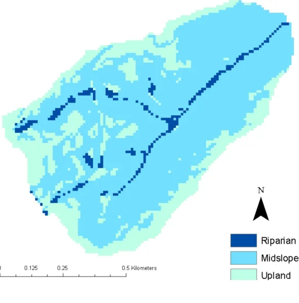
applied without modification. Soil default files were adapted from the library file for sandy loams and modified to reflect the variability in soil properties with topographic position. Based on field observations, catchment soils were classified into 3 classes: riparian, midslope, and upland. Riparian soils were assigned a soil depth of 8 m, soil porosity of 0.485, and pore size index of 0.589; midslope soils were assigned a soil depth of 1 m, soil porosity of 0.485, and pore size index of 0.189; and upland soils were
assigned a soil depth of 15 m, soil porosity of 0.435, and pore size index of 0.204 following Law (2004).
d.
Streamflow time series
Daily discharge from BR3 was estimated based on the regression of synoptic samples taken at the outlet against USGS data for BR. Twenty four synoptic samples of discharge from BR3 were collected between July 2001 – January 2003 and August 2006 – October 2007. Corresponding flows from BR were obtained from the USGS database, and discharges from the two locations were plotted against one another (Figure 4.5). Though the measurements at larger discharges suggest that the data might best be characterized by a power function, the number of samples was considered inadequate to determine the power function coefficients, and a linear relationship was assumed. Linear regression was performed on the thirteen synoptic samples collected between 7/2001 and 1/2003 measuring discharges of less than 555 m3/day (or 0.80 mm/day). The slope of the best fit line between volumetric discharge from BR3 and BR was 0.21, a figure quite close to the ratio of catchment areas (0.18). It is therefore probable that estimates of discharge from BR3 are more accurate for low and moderate flows than for high flows, and may underestimate high flows.
34
measurements at high flows were available, the linear relationship observed at low flows was assumed to characterize high flows as well. Several synoptic samples at somewhat higher flows, however, suggest that the relationship between discharge from BR3 and discharge from BR might be better approximated by a power function. It is because of this severe limitation to the accuracy of our estimates of streamflow from BR3 that a proxy-catchment approach is applied to calibrate the model for BR3. Though
7.
Methods
a.
Spatial Data Processing
Extensive processing was conducted to translate the GIS datasets described above into the landscape and flowpath representations required by RHESSys. Spatial data processing used 3 programs: the Terrain Analysis System (TAS), ESRI ArcMap, and the RHESSys utility CREATE_FLOWPATHS. Prior to all processing described below, the source datasets were resampled to 10 m resolution. This aggregation was required to reduce the quantity of computational units to a number that would not exceed dedicated computational resources.
i.
Catchment Delineation
For both catchments, we first coarsened the 1 m LIDAR dataset described above to a 10 m digital elevation model (DEM), then used TAS to derive the catchment
36
mapped by the county. The best approximations were derived with a specific
contributing area threshold of 450 m2, and a stream length threshold of 180 m. Figure 4.6 shows derived catchment boundaries and stream networks, along with the stream
channels mapped by the county. TAS was also used to derive hillslope boundaries based on the DEM and derived channel networks. Delineation generated three hillslopes for PB, and twenty hillslopes for BR3. Derived hillslope boundaries are shown in Figure 4.7.
ii.
Catchment Topography and Soils
To generate a landscape representation for each catchment, RHESSys required maps of catchment slope, aspect, and wetness index, as well as elevation. Functions provided by TAS were used to generate each of these layers from the 10 m DEM. As noted in the descriptions of the study area and default files, soils in both catchments are observed to vary significantly with topography. Because the soil coverages provided by SSURGO were of insufficiently fine resolution to represent the variation of catchment soils with topography, catchment topographic layers were processed to produce a layer describing the distribution of soil types. A simple conceptual model was constructed to classify catchment soils into 3 classes: riparian, midslope, and upslope. Riparian soils were predicted to occur in areas of low slope within a small distance of the stream channel, while upland soils were predicted to occur in areas of low slope beyond a small distance from the stream channel, and midslope soils were predicted to occur in all other areas. To translate this conceptual model into a representation of catchment soil
stream channel were classified as upland, and all other cells were classified as midslope (Figure 4.8). Though approximate, the resulting classifications were in accord with expert knowledge of the catchments.
iii.
Catchment Land Use and Land Cover Layers
Coverages of land use, land cover, and vegetation characteristics were derived from the 5 m land cover classification map provided by Zhou and Troy (2006). To generate a coverage of land use, we reclassified building and pavement as urban and all vegetation as undeveloped. Similarly, to generate a coverage of land cover we
reclassified building and pavement as impervious, fine textured vegetation as grass, and coarse textured vegetation as forest. Figure 4.3 shows the resulting map of land cover for BR3. According to this map, land cover in BR3 consists of ~65.3% (or 45 ha) forest, ~7.3% (or 5 ha) impervious surface, and ~ 27.3% (or 18.7 ha) lawn.
To describe vegetation characteristics, RHESSys requires maps of rooting depth and leaf area index (LAI). To generate a coverage of rooting depth, we assigned building and pavement land covers a rooting depth of 0, fine-textured vegetation a rooting depth of 8 cm, and coarse-textured vegetation a rooting depth of 1 m. Because no field
measurements were available, we applied order of magnitude estimates based on a review of the literature. Studies report a mean rooting depth for temperate deciduous forests of 2.9 ± 0.2 m (Canadell et al.,1996), while turfgrass scientists report a typical rooting depth for cool-season turfgrasses of 5 – 15 cm (Landschoot 2007, Lilly personal
38
coverage of LAI, we initially assigned building and pavement a maximum LAI of 0, fine-textured vegetation a maximum LAI of 0.5, and coarse-fine-textured vegetation a maximum LAI of 5. Field measurements of leaf litter in the BES permanent plots suggested an all-sided LAI of 10, and therefore a one-all-sided LAI of 5. Again, because no field
measurements were available for grass LAI, we applied an order of magnitude estimate based on values published in the literature (Lazzaroto et al. 2009). Initial calibration results for PB and BR3 (described further below) suggested that LAI values for PB forest canopy might be lower than those for BR3. These results corresponded with field
observations of the tree canopy in the 2 catchments. In Pond Branch, greater damage to the tree canopy was observed following Hurricane Isabel, and the overstory along the riparian corridor was observed to be poorly developed relative to the overstory in BR3. PB LAI values for coarse textured vegetation were therefore modified to 4.5 for midslope and upland locations, and 2.5 for riparian locations. For urban catchments, RHESSys also requires a coverage defining the extent of impervious surface. To generate a
coverage of impervious surface, we reclassified building and pavement as impervious and all other land covers as pervious.
iv.
Catchment Flowpaths
b.
Calibration and Validation
Calibration and validation of RHESSys to simulate land cover change in BR3 was complicated by all three obstacles discussed in Sections 2d, 2e, and 2f. First, limited streamflow data were available to calibrate the model. As discussed above, the availability of streamflow data for BR as well as a set of instantaneous streamflow measurements for BR3 permitted the estimation of daily discharge (Q) from BR3, but the linear relationship developed was observed to perform poorly at higher flows. We therefore applied the first approach to model calibration in the absence of data presented in Section 2d, and calibrated RHESSys for data from PB. The model was calibrated for data from October 1, 2004 to September 30, 2005 and October 1, 2006 to September 30, 2007 (analysis of seasonal precipitation and discharge data suggested that precipitation data for water year 2006 was inaccurate). Five parameters were calibrated: a parameter describing the exponential decay of hydraulic conductivity with depth (m), a multiplier for saturated hydraulic conductivity in the horizontal dimension (Ksat0), a multiplier for
saturated hydraulic conductivity in the vertical direction (Ksat0,v), a parameter describing
40
measures for each parameter set. We calculated the Nash Sutcliffe efficiency of Q to measure the accuracy of peak flow predictions, and the Nash Sutcliffe efficiency of log(Q) to measure the accuracy of baseflow predictions. All parameter sets for which the Nash Sutcliffe efficiency of both Q and log(Q) were greater than 0.5 were designated behavioral.
The second obstacle complicating model calibration and validation was the absence of streamflow data collected across a change in land cover. As discussed above, model predictions may be regarded as reliable only when model validation has
demonstrated the model’s fitness for its intended application. For this research, model validation must demonstrate the model’s ability to accurately predict streamflows for different land covers. Though insufficient data was available for a differential split-sample test, sufficient data was available for a limited proxy-basin test. At low flows, the linear regression of streamflow from BR3 against streamflow from BR was observed to produce accurate estimates of streamflow from BR3. Low flows from BR3 were
forested Pond Branch catchment and validating model parameters with low flows from the suburban Baisman Run 3 catchment, we achieved a limited proxy-basin test.
The third obstacle complicating model calibration and validation was the uncertainty derived from model errors, input data errors, output variable errors, and parameter uncertainty. This research uses the GLUE methodology to generate
42
runoff volume, for Pond Branch the Nash Sutcliffe efficiencies of Q were selected for inclusion in the likelihood measure. Because estimates of high flows from BR3 were of limited accuracy, for BR3 the NS efficiencies of log(Q) were selected for inclusion in the likelihood measure. Beven (2001) identifies summation and multiplication as appropriate operations to combine likelihood measures. For this research, the likelihood measure was calculated as the product of NS(Q) for Pond Branch and NS(logQ) for BR3, normalized so that the sum of all measures for all behavioral parameter sets was 1.
c.
Simulation of Vegetation Management Practices
Three vegetation management practices were simulated in Baisman Run 3: conversion of all lawn to forest, conversion of downslope lawn to forest, and conversion of upslope lawn to forest. To generate the first scenario, all 18.65 haof lawn were converted to forest. To generate the second and third scenarios, the lawn was partitioned into equal areas based on upslope contributing area. The value of the upslope
8.
Calibration and Validation Results
a.
Calibration
As discussed above, model parameters were calibrated for Pond Branch by comparing the simulated streamflows produced by randomly-generated parameter sets to the observed streamflow recorded at Pond Branch. Initial calibration results assuming a forest LAI of 5.0 yielded no behavioral parameter sets (defined as having NS>0.5 for both Q and log(Q)). Initial calibration achieved a maximum Nash Sutcliffe efficiency for Q of 0.47, and a maximum Nash Sutcliffe efficiency for log(Q) of 0.53. The range of predicted streamflows for all parameter sets with NS efficiencies > 0.4 indicated that the model consistently underpredicted streamflows (Figure 5.1). The consistent
underprediction of streamflow suggested an overprediction of ET and LAI. Forest LAI values were therefore adjusted to 4.5 in upland areas and 2.5 in riparian areas, and the calibration simulations were repeated.
The adjustment of Pond Branch LAI values significantly improved streamflow predictions. Calibration results yielded 193 behavioral parameter sets (defined as having NS>0.5 for both Q and log(Q)). Calibration achieved a maximum Nash Sutcliffe
efficiency for Q of 0.56, and a maximum Nash Sutcliffe efficiency for log(Q) of 0.60. Figures 5.4a, b, and c compare the range of predicted streamflows to the observed
observations for a much greater proportion of the simulation period. Field measurements of LAI should be collected to better constrain model values.
b.
Validation
Model validation transferred the parameter sets calibrated for Pond Branch to Baisman Run 3. For the performance criteria described above, model validation yielded 92 behavioral parameter sets. Interestingly, goodness of fit results for validation often exceeded those for calibration (Figure 5.2). Validation achieved a maximum Nash Sutcliffe efficiency for Q of 0.71, and a maximum Nash Sutcliffe efficiency for log(Q) of 0.68. Prior and posterior distributions of the parameters to which model performance was most sensitive are shown in Figure 5.3.
Comparisons of the range of predicted discharges to the observed (for PB) and estimated (for BR3) discharges are shown in Figures 5.4a, b, and c and 5.5a, b, and c. Though the observed/estimated discharge is not consistently bounded by the predicted range for either PB or BR3, the model generally reproduces the trends in discharge very well. The most significant deviation between the model predictions and the
observed/estimated discharges occurs in July and August of 2007, when the
46
underestimates of the actual values. Because July and August of 2007 were very dry months, it may also be that the study streams experience transmission losses in extremely dry conditions which the model algorithms cannot reproduce. Interestingly, the model appears to perform better for the suburban validation catchment than for the forested calibration catchment.
Bias and mean absolute error (MAE) were calculated for the expected value of daily discharge from PB and BR3 (obtained by taking the weighted average of simulated discharge for each behavioral parameter set). While PB simulated discharge exhibited a downward bias of 0.2 mm/day (or ~14% of the mean daily discharge of 1.47 mm), BR3 simulated discharge exhibited an upward bias of 0.17 mm/day (or ~14% of the mean daily discharge of 1.24 mm). Mean absolute errors were comparable for PB and BR3, with a MAE of 0.32 for PB and 0.35 for BR3.
Figure 5.6 presents the difference between simulated expected discharge and observed daily streamflow for each catchment. For both catchments, the model underpredicts peak flows. The difference in the direction of model bias is observed to derive from simulated baseflows. For PB, the model underpredicts baseflows, while for BR3 the model overpredicts baseflows.
9.
Vegetation Management Results
a.
Impact of Vegetation Management on Streamflow Regime
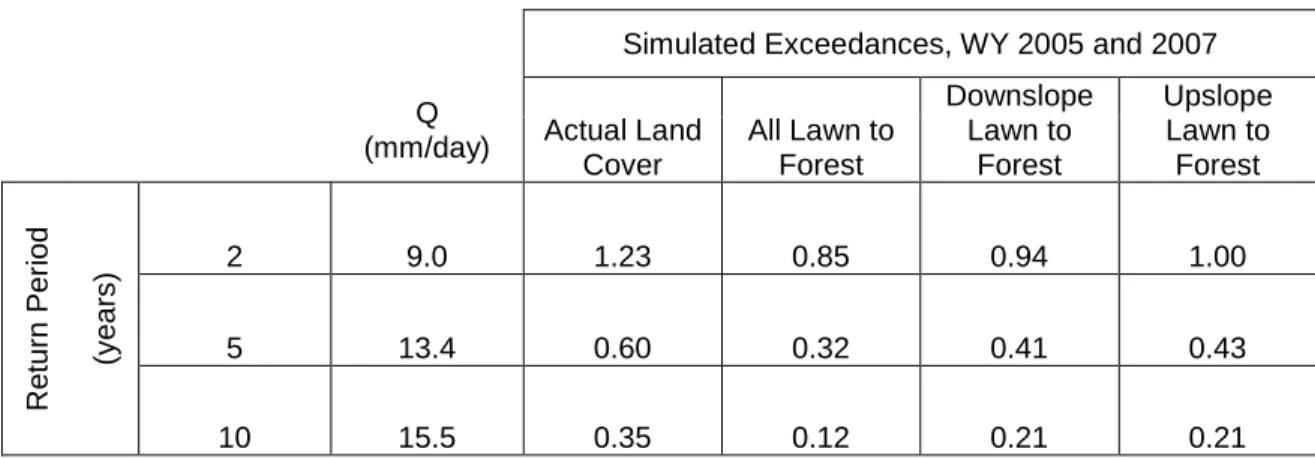
Both runoff volumes and peak flows declined dramatically with the conversion of some or all of the lawn area in BR3 to forest. Annual runoff volumes fell ~100 mm (or 20%) when all lawn was converted to forest and ~50 mm (or 11%) when half the lawn area was converted to forest (Figure 5.7). To examine the impact of vegetation
management on peak flows, we estimated the 2, 5, and 10 year flows given the actual land cover. We fitted a Log Pearson Type III distribution to the annual peak flows for water years 2000-2008. To estimate the flows that occur with recurrence intervals of 2, 5, and 10 years, we applied the following equation:
Q
K X
Q) log
log( = + σ , (3)
where Q is the flow magnitude at the selected recurrence interval, X is the average of the logarithms of the available peak flows, K is a frequency factor that is a function of the skewness coefficient and recurrence interval, and σ is the standard deviation of the
number of exceedances for each behavioral parameter set by the corresponding likelihood measure. Exceedances of all examined flows fell most when all lawn was converted to forest, less when the downslope lawn area was converted to forest, and even less when the upslope lawn area was converted to forest (Table 5.1).
50
storms of 10 - 65 mm per day account for most of the cumulative depth of precipitation. Interestingly, the frequency of the largest storms (greater than 50 mm per day) is
comparable for all seasons. Though precipitation in the Baltimore region is generally delivered by less intense frontal storms in the winter and more intense convective storms in the summer, seasonal differences in storm intensity are not perceived at the daily scale. These patterns in seasonal streamflow, runoff ratio, and precipitation indicate that
evapotranspiration is a key mechanism shaping catchment hydrologic response.
and spring, while baseflows from the forested-upslope scenario are greater during the summer.
b.
Sensitivity of Predicted Streamflow to Estimated Root Depth
Limited analysis of the sensitivity of streamflow results to the definition of grass rooting depth indicated that the above conclusions are robust across a range of rooting depths. Figure 5.11 compares simulated monthly discharge for the entirely forested scenario, the actual scenario with shallow grass roots (8 cm), and the actual scenario with deep grass roots (30 cm). For both deep and shallow grass root depths, monthly
discharge is predicted to be significantly lower for the entirely forested scenario than for the actual scenario, with the difference greatest in the summer, fall, and winter and least in the spring. The sensitivity analysis also suggested that the unexpected dependence of streamflow response on the topographic position of catchment vegetation is robust across the range of rooting depths examined. Figure 5.12 shows the difference between monthly discharge from the forested upslope scenario and monthly discharge from the forested downslope scenario for both shallow and deep grass roots (compare to Figure 5.10). For deep grass roots as well as shallow grass roots, streamflows from the forested downslope scenario are greater in the fall and winter, while streamflows from the forested upslope scenario are greater in the summer.
c.
Impact of Vegetation Management on Evapotranspiration
52
differences in discharge. ET increases dramatically with the conversion of some or all lawn area to forest. Annual ET for the 4 vegetation management scenarios is shown in Figure 5.13. Note that the change in annual ET when lawn is converted to forest exceeds the change in annual discharge. ET increases by ~150 mm when all lawn area is
converted to forest, and by ~75 mm when half the lawn area is converted to forest. The topographic position of re-forested areas does not appear to have a significant impact on annual ET.
As with streamflow, seasonal trends are apparent in the response of ET to the various vegetation management scenarios. Differences in monthly ET among the 4 scenarios are greatest in the growing season and negligible in the winter and fall, suggesting that transpiration accounts for most of the difference in ET (Figure 5.14). Comparison of changes in monthly evaporation to changes in monthly transpiration when lawn area is converted to forest confirms the dominance of transpiration (Figure 5.15a, b). Note that while evaporation is enhanced throughout the year, transpiration is enhanced only between the months of May and October. At the monthly scale as well, topographic position of re-forested areas does not appear to have a significant impact on ET.
4.8, it is observed that decreases in ET are greatest in the riparian areas. Note that the extent of areas experiencing decreased ET is greater for the forested-downslope scenario than for the forested-upslope scenario.
d.
Impact of Vegetation Management on Soil Moisture
As expected, simulation results indicated that catchment-average saturation deficit is significantly altered by vegetation management. Figure 5.17 shows daily average saturation deficit for the entirely forested and actual scenarios. The increase in saturation deficit associated with re-forestation is more persistent in time than the increase in ET. While ET from the entirely forested scenario exceeds ET from the actual scenario only in the spring and summer, saturation deficit for the forested scenario exceeds saturation deficit for the actual scenario throughout the year. During the months in which ET from the forested scenario exceeds ET from the actual scenario, the difference in saturation deficit between the two scenarios is observed to increase. Conversely, during the months in which ET from the forested scenario is equivalent to ET from the actual scenario, the difference in saturation deficit between the two scenarios is observed to decline.
Unexpected differences are also observed in the temporal patterns of soil moisture for the forested-downslope and forested-upslope scenarios. Figure 5.18 shows the
54
scenario often has a larger saturated area. In all 4 seasons the forested upslope scenario has a greater saturation deficit than the forested-downslope scenario, but the difference declines throughout the fall, winter, and early spring, and rises in the late spring and summer. The timing of these differences appears to correspond to the timing of the differences in daily streamflow for the two scenarios (5.14 top pane). During the months in which the upslope scenario produces less baseflow than the
forested-downslope scenario, the forested-upslope scenario also has a smaller saturated area. Conversely, during the months in which the forested-upslope scenario produces more baseflow than the forested-downslope scenario, the forested-upslope scenario also has a greater saturated area. A similar correspondence is observed for the differences in daily average saturation deficit. During the months in which the saturation deficit of the two scenarios is converging, the forested-upslope scenario produces less baseflow than the forested-downslope scenario. Conversely, during the months in which the saturation deficit of the two scenarios is diverging, the forested-upslope scenario produces more baseflow than the forested-downslope scenario.
Figures 5.19 and 5.20 present maps of saturation deficit for two dates on which storms occurred: December 15, 2005 (when the catchment received ~45 mm of
precipitation) and July 8, 2005 (when the catchment received ~60 mm of precipitation). In these figures ACT denotes actual land cover, FA denotes the conversion of all forest to lawn, FD denotes the conversion of downslope forest to lawn, and FU denotes the
10.
Discussion
This section begins with a discussion of the results and their relevance to land use planning in the context of the research questions, and concludes with a review of the research limitations.
a.
Research Questions
Question A1: Can calibrated soil and groundwater parameters from a forested reference
catchment be transferred to an ungauged suburban catchment?
Goodness-of-fit results for BR3 suggest that the transfer of parameters from a forested to a lightly urbanized catchment is viable, though neglecting the dependence of soil parameters on land cover may degrade model performance. While Nash Sutcliffe results suggest that the accuracy of model predictions for BR3 exceeds the accuracy of model predictions for PB, daily bias results indicate that the transfer of soil and
groundwater parameters from a forested to an urbanized catchment may introduce error into the urban model. Potential sources of model bias include errors in the model structure and errors in the model parameters. We note that much of the model bias may be explained by errors in the LAI, hydraulic conductivity, and groundwater bypass parameters. In Pond Branch, the overestimation of LAI would explain the
hydraulic conductivity and groundwater bypass parameters might explain the underprediciton of peak flows and overprediction of baseflows. Indeed, previous research suggests that we likely overestimated the hydraulic conductivity and
groundwater bypass parameters in BR3 by assuming these parameters to be independent of land cover. Field studies of infiltration rates in urban areas have found that urban soils are generally more compacted than undisturbed soils and tend to infiltrate water at lower rates (Gregory et al. 2006, Pitt et al. 2001, Hamilton and Waddington 1999). By transferring soil and groundwater parameters from a forested to an urbanized catchment without modifying parameter values to reflect the change in land cover, we likely overestimated the values of the hydraulic conductivity and groundwater bypass parameters. Though we cannot provide conclusive evidence that errors in these
parameters are the source of model bias in BR3, our preliminary assessment indicates that this explanation is consistent with both field studies and model results.
58
personal communication). We therefore propose that the viability of parameter transfer from forested to urbanized catchments may be dependent on the extent of urbanization, and recommend that this technique be examined further in more highly urbanized catchments.
Question A2: Can a distributed, physically based model accurately reproduce streamflow
from a suburban catchment?
The goodness-of-fit results for BR3 suggest that distributed, physically based models are not only capable of reproducing streamflow from suburban catchments, but may perform better in suburban catchments than in forested catchments. This result is consistent with previous studies of the application of distributed, physically based models to urbanized catchments, which determined that model performance in urbanized
This result and our parameter transfer results above offer a promising approach to the problem of predicting the impacts of land cover change in data-sparse urban areas. While parameter transfer schemes among catchments with similar physical characteristics can compensate for the lack of calibration data in urban areas, distributed, physically based models can provide distributed predictions of the impacts of land cover change and greater insights into the mechanisms producing those impacts. Further research should be conducted to develop and demonstrate this promising methodology.
Question B1: What is the impact of different extents of tree cover in a suburban
catchment on aggregate catchment response? Does this impact exceed the uncertainty generated by parameter uncertainty?
Our study supports previous findings that the extent of forest and lawn in
60
response, and that modest increases in catchment LAI produce significant decreases in annual runoff (~20% per unit change in catchment LAI). Moreover, by comparing the changes in streamflow response to the prediction bounds of the behavioral parameter sets, we demonstrate that the change in streamflow response associated with different extents of vegetation cover exceeds the uncertainty associated with parameter estimation.
This result has significant implications for land use planning. We demonstrate that expanding the urban tree canopy is an effective approach to reducing runoff volumes and peak flows from suburban catchments. Given the well established connection
between flow regimes and stream channel erosion, pollutant delivery, and habitat
degradation, we interpret this result to suggest that the expansion of the urban tree canopy is an effective approach to mitigating the symptoms of urban stream syndrome. This interpretation agrees with the results of previous empirical studies demonstrating the importance of tree cover as a predictor of stream biotic integrity (Hammer 1972, Goetz and Fiske 2008, Carlisle and Meador 2007, Strayer 2003, Steedman 1988).To attain water quantity and quality goals, land use planners should preserve or plant as much tree cover in urban areas as is consistent with other community goals.
Question B2: What is the impact of different patterns of tree cover in a suburban
Our analysis of the impact of the topographic position of tree cover on streamflow response produced unexpected results with complex implications for land use planning. Though the planning literature generally recommends the planting or preservation of riparian forests to minimize the ecological impacts of urbanization, we found that riparian forests may not provide greater mitigation of the hydrologic impacts of urbanization than upslope forests. At the annual scale, the conversion of upslope lawn to forest actually reduced streamflow more than the conversion of downslope lawn to forest, while at the seasonal scale the conversion of upslope lawn to forest produced greater reductions in streamflow in 3 of 4 seasons. At the daily scale, however, the interpretation of our results becomes more complex. Though the conversion of upslope lawn to forest produces lower baseflows than the conversion of downslope lawn to forest, it consistently produces higher peak flows. Because both the reduction of peak flows and the reduction of runoff volumes are goals of stormwater management, this result requires a tradeoff among management goals. We propose that the management strategy most protective of ecosystem function may depend on the relative sensitivity of channel morphology and stream biota to erosive peak flows versus amplified baseflows, and the pollutant loads of each.