ESSAYS IN INTERNATIONAL ECONOMICS USING FIRM-LEVEL DATA
Jennifer S. Rhee
A dissertation submitted to the faculty of the University of North Carolina at Chapel Hill in par-tial fulfillment of the requirements for the degree of Doctor of Philosophy in the Department of
Economics.
Chapel Hill 2018
c
2018
ABSTRACT
JENNIFER S. RHEE: ESSAYS IN INTERNATIONAL ECONOMICS USING FIRM-LEVEL DATA.
(Under the direction of Anusha Chari)
My dissertation empirically investigates implications of macroeconomic models using firm-level market and accounting data. As Konchitchki and Patatoukas (2014) states, ”macroeconomics research has evolved independently from accounting research, which is typically conducted at the firm level” and ”the link between accounting earnings and macroeconomy remains relatively unexplored.” This paper is part of the growing body of literature that attempts to fill this gap by highlighting macroeconomic insights that can be obtained from the micro-level analysis. The first two chapters of my dissertation investigate Lucas Paradox and the neoclassical model, and the last chapter studies Heckscher-Ohlin model of trade.
efficiency to explain the observed patterns of financial returns. The second chapter further inves-tigates capital efficiency differences across countries and suggests potential modifications to the standard capital accumulation model. It also uses variables that are commonly employed in the macroeconomic growth literature and examine their effect on the capital efficiency of firms.
ACKNOWLEDGMENTS
TABLE OF CONTENTS
LIST OF TABLES . . . viii
LIST OF FIGURES . . . x
1 The Lucas Paradox and the Return to Capital in Capital-Scarce Countries . . . 1
1.1 Introduction . . . 1
1.2 Benchmark model and Empirical Methodology . . . 7
1.2.1 Benchmark: Neoclassical model . . . 7
1.2.2 Empirical Methodology . . . 9
1.3 Data and Summary Statistics . . . 12
1.4 Cross Country Marginal Products of Capital and Investment Return Patterns . . . . 17
1.4.1 Firm-Level Return on Assets and Per Capita GDP . . . 17
1.4.2 Investment Returns and Per Capita GDP . . . 21
1.5 Additional Test and Robustness Checks . . . 24
1.5.1 Robustness Check: Hourly labor input . . . 25
1.5.2 Robustness Check: Tax adjusted income . . . 26
1.6 Conclusion . . . 28
2 The Lucas Paradox and the Capital Accumulation in Capital-Scarce Countries . . . 42
2.1 Introduction . . . 42
2.2 Benchmark Model and Empirical Methodology . . . 45
2.2.1 Benchmark Model and Modifications . . . 45
2.3 Data . . . 49
2.4 Modified Capital Accumulation Model . . . 50
2.4.1 Testing Modified Capital Accumulation Model . . . 50
2.4.2 Macroeconomic factors . . . 51
2.5 Conclusion . . . 54
3 Multi-Cone Evidence From the Firm-Level Data . . . 60
3.1 Introduction . . . 60
3.2 Benchmark Model: Heckscher Ohlin model of Comparative Advantage . . . 63
3.3 Empirical Methodology and Data . . . 65
3.3.1 Empirical Methodology . . . 65
3.3.2 Data Descriptions . . . 66
3.4 Single vs. Multi-cone Heckscher Ohlin Model . . . 68
3.5 Technology Difference vs. Product Specialization . . . 70
3.5.1 Alternative Explanation: Technology Differences . . . 70
3.5.2 Specialization Within vs. Across Industries . . . 71
3.6 Conclusion . . . 72
A Chapter 1 Appendix . . . 80
B Chapter 3 Appendix . . . 90
LIST OF TABLES
1.1 Data Summary Statistics (1997-2014) . . . 30
1.2 Summary Statistics: ROA vs. IRR (1997-2014) . . . 31
1.3 MSCI Developed and Emerging Countries: Firm ROA and PCGDP . . . 32
1.4 Non-Financial 48 Fama French Industries: Firm ROA and PCGDP . . . 33
1.5 Annual Analysis: Firm ROA and PCGDP . . . 34
1.6 MSCI Developed and Emerging Countries: Firm Investment Return and PCGDP . 35 1.7 Non-Financial 48 Fama French Industries: Firm IRR and PCGDP . . . 36
1.8 Annual Analysis: Firm IRR and PCGDP . . . 37
1.9 Robustness Check: log(PHGDP) vs. ROA and IRR . . . 38
1.10 Robustness Check: Tax Adjustment . . . 39
2.1 Summary Statistics: Capital Friction and Investment-Capital Ratio . . . 56
2.2 Testing Capital Accumulation Path . . . 57
2.3 Macroeconomic Factors Summary Statistics . . . 58
2.4 Macroeconomic factors and Capital Efficiency . . . 59
3.1 Data Summary Statistics (1997-2014) . . . 75
3.2 ROA vs. log (PCGDP) . . . 76
3.3 Turnover vs. log(Per capita GDP) . . . 77
3.4 Countries by SIC 2-Digit Manufacturing Industries (2014) . . . 78
3.5 Manufacturing: ROA vs. log(PCGDP) . . . 79
A.1 Accounting Standard and IFRS Adoption Date by Country . . . 81
A.2 Firm and Country Fixed Effects: MPK and IRR for 1996-2014 . . . 82
A.4 Non-Financial 2-digit SIC Industries: Firm ROA and PCGDP . . . 84
A.5 Non-Financial 2-digit SIC Industries: Firm IRR and PCGDP . . . 87
B.1 ROA vs. log(Per Capita Capital) . . . 90
B.2 Turnover vs. log(per capita Capital) . . . 91
LIST OF FIGURES
1.1 ROA and IRR distribution plot . . . 40
1.2 ROA and IRR scatter plot . . . 41
3.1 Lerner Diagram . . . 74
CHAPTER 1
THE LUCAS PARADOX AND THE RETURN TO CAPITAL IN CAPITAL-SCARCE COUNTRIES
1.1 Introduction
Textbook neoclassical theory predicts that if two countries share identical production functions, and trade in capital goods is free and competitive, new investment will only occur in economies with relatively less capital. It follows from the law of diminishing returns that the marginal product of capital ought to be higher in capital-scarce economies. However, since Lucas (1990) a vast literature devotes itself to explain the observation that capital flows from developed to emerging countries fall short of what theory predicts. In fact, in their 2007 paper, Prasad, et al., document an uphill flow of capital from poor to rich countries in the late 1990s-early 2000s. So, why doesn’t capital flow from developed to developing countries?
In this essay, I investigate the link between the marginal product of capital and financial rates of return to provide resolution to the paradoxical patterns of observed international capital flows. In the standard neoclassical model, a firm’s first order condition states that the marginal product of capital (M P Kt) and the financial return (rt) should differ only by depreciation rate (δ), which is
assumed constant across countries (rt =M P Kt−δ). Therefore, theory predicts that high financial
returns and high marginal products of capital should go hand in hand. If this link breaks down, i.e., if high marginal product of capital does not translate to high financial returns, it is not clear that the capital ought to flow to countries with high marginal products of capital.
evolved independently from accounting research, which is typically conducted at the firm level” and ”the link between accounting earnings and macroeconomy remains relatively unexplored.” This essay is part of the growing body of literature that attempts to fill this gap by highlighting macroeconomic insights that can be obtained from the micro-level analysis.
The standard approach in recent work imputes an aggregate marginal product of capital from national income accounts. However, imputed estimates are not the same as computed ones. Impu-tations rely heavily on underlying assumptions about functional form, raising legitimate questions about the validity of a range of assumptions such as setting parameter values (e.g., technology, capital shares, and elasticities of substitution) equal to those of the US. Specifically, delivering the finding that marginal products of capital are essentially the same across rich and poor countries requires adjustments to the national income accounts for (i) the capital per effective worker and a human capital externality (Lucas, 1990), (ii) non-reproducible capital and the price of capital goods (Caselli and Feyrer, 2007), and (iii) technology catch up and distortions in saving and investment decisions (Gourinchas and Jeanne, 2009).
Imputed estimates are therefore indirect estimates of the aggregate rate of return to capital in developing countries. On the other hand, computed estimates of the return to capital using micro-data may provide a more direct and reliable way forward. Instead of making assumptions about parameters to impute the rate of return to capital from aggregate data, I argue that it is more straightforward to compute firm-level rates of return and to aggregate them to produce estimates of the national rate of return.
The main finding of this paper is that the standard link between the marginal product of capital and the financial return, that is often assumed in the international capital flows literature, does not hold across in a sample of developed and emerging countries between 1997-2014. Consistent with predictions from the neoclassical framework, the results show that firm marginal products of cap-ital are indeed higher in emerging countries relative to their developed-market counterparts. The finding is robust to controlling for firm and industry specific effects and is remarkably consistent across different sample periods and countries.
high financial return in emerging-markets. However, contrary to this prediction, I find that despite evidence for a downward sloping marginal product of capital curve, the inflation-adjusted financial return is roughly equal across developed and emerging countries. This core finding is significant as it questions the validity of the standard approach that uses differences in the marginal product of capital to explain international capital flow patterns. The firm-level evidence using computed estimates therefore shows that the marginal product of capital may not be a valid proxy for financial returns expected from the capital investment.
Additionally, the results confirm that ”there is no prima facie support for the view that inter-national credit frictions play a major role in preventing capital flows from rich to poor countries” (Caselli and Feyrer, 2007). If a high marginal product of capital in emerging countries correctly translates to high financial returns as implied by the standard model, then the shortfall in the capital flow to these countries points international capital market frictions and investment barriers. How-ever, if financial returns are equalized across developed and emerging countries, an alternative hypothesis may be that there is little incentive for capital to flow to the less-developed countries.
These findings further highlight the importance of cross-country capital efficiency differences to explain the Lucas Paradox. Much of the international macro and growth literature, which uses cross-country marginal product of capital differences to explain international capital flow patterns, focuses on productivity differences across countries and the macroeconomic factors that affect productive efficiency, i.e., the level of output that can be obtained from a unit of the capital input. The findings of this paper highlight the importance of capital efficiency, i.e., the level of future capital input that can be obtained from a unit investment today. This relationship affects the capital accumulation process within the economy and determines the relationship between the marginal product of capital and financial returns.
The firm’s first order condition that links the marginal product of capital and financial returns stems from the standard capital accumulation equation, which suggests that the capital stock to-morrow is the sum of capital stock today and the investment net of the depreciation (Kt+1 =
(1−δ)Kt+Itsuch thatKtandItare the capital stock, and investment in periodt, respectively).
link between the investment return and marginal product of capital no longer holds, and the cross-country investment return and marginal product of capital patterns can differ.1
As Alfaro, et al (2008) states, “theoretical explanations for the Lucas Paradox can be grouped into two categories. The first group includes differences in fundamentals that affect the produc-tion structure of the economy, such as technological differences, missing factors of producproduc-tion, government policies, and the institutional structure. The second group of explanations focuses on international capital market imperfections, mainly sovereign risk and asymmetric information.” Some of the major works on international capital market frictions include Stulz (2005), which shows that agency problems in emerging countries can lead to a wedge in the investment returns received by the international and domestic investors, and Reinhart and Rogoff (2004), which high-lights the default history of emerging market countries. This finding suggest that the credit risk can explain the paucity of capital flow to emerging countries. Montiel (2006) also proposes an in-formation friction as an important determinant in explaining the paucity of capital flows to African countries. On the other hand, much of the international macro and growth literature, which uses cross-country marginal product of capital differences to explain international capital flow patterns, focus on macroeconomic fundamentals and endowments that affect productive efficiency.2
In their 2005 paper, Banerjee and Duflo outline an exhaustive list of indirect and direct meth-ods used to calibrate the marginal product of capital in the empirical development literature. An indirect method often employed in the literature proxies for the firm return to capital using the in-terest rate. Therefore a long line of researchers study of lending market in the emerging countries, and they document the extremely high cost of borrowing in these countries even when one adjusts for the risk. For example, Timberg and Aiyar (1984) document a21−120%interest rate charged by the indigenous-style bankers in India, and Ghate (1992) shows that interest rates in northern Thailand range up to5−7%per month.
However, as stated in Caselli and Feyrer (2007), “in financially repressed/distorted economies, interest rates on financial assets may be very poor proxies for the cost of capital actually borne
1See Cochrane (1991), Hayashi (1982), and Abel and Blanchard (1986)
by firms.” More popular and direct estimates of marginal product of capital require one to posit a production function (usually Cobb-Douglas) and derive the expression for marginal product of capital based on the assumed equation. This is the approach employed by Lucas in his 1990 paper, and he shows that marginal product of capital difference across countries fall substantially when one adjust for productivity difference across countries. A more recent paper by Caselli and Feyrer (2007) finds that the return to capital is roughly equal between emerging and developed countries when one adjusts for the relative price of capital, and the complementary factors of production.
Within this extensive literature on Lucas Paradox, there has been a relatively little discussion about the link between the marginal product of capital and the investment return. In large part, this is because in aggregate data, capital is not observed and therefore estimated from aggregate investment using the perpetual inventory method, which requires one to posit a capital accumu-lation process. Since this process is typically assumed to follow a standard model where a unit increase in investment lead to a unit increase in capital stock3, the aggregate capital stock estimate itself implicitly relies on the assumption that the standard link between marginal product of capital and the investment return holds. This makes it virtually impossible to test the validity of the link using aggregate data. The key advantage of a firm-level data is that unlike aggregate estimates, capital can be directly observed from the accounting and market values. This allows for direct computation of the marginal product of capital and investment returns, which can then be used to empirically test the validity of the standard link between the two variables.
Despite the advantages of firm-level data, there are some drawbacks. For example, firm-level data do not provide any insight into the productivity of self-employed workers or informal sector firms. This is a significant drawback as these types of households and firms constitute a large part of the economy in developing countries. Unlike aggregate data, firm-level market variables are also susceptible to market volatility. Since the period of analysis includes the global financial crisis (2007-2008), I control for year-specific effects in my analysis and also run a robustness test
3Cochrane (1991) is an exception in that he uses non-standard capital accumulation process with adjustment cost
excluding these years. Despite these shortcomings, the firm-level data provide useful insights as they utilize detailed information on the relationship between financial returns and productivity of the firms. This paper therefore provides an alternative lens to complement existing literature that primarily uses macroeconomic data to perform aggregate analysis.
The paper limits the analysis to listed-firms in MSCI emerging and developed countries that have relatively well established stock markets. Although this substantially reduces the number of countries in the sample, as Reinhart and Rogoff (2004) write ”roughly twenty five ’emerging markets’ account for the bulk of international financial flows.” Therefore, the analysis of the firms in these countries ought to provide useful insights into the factors that drive the international capital flows. I also restrict the period of analysis to the post-1996 period due to the limited availability of reliable firm-level data from emerging countries in the early 1990s.
An important concern with using cross-country firm-level data is the difference in the account-ing standards used to report data from different countries. For example, the definition of ”assets” in the US Generally Accepted Accounting Principles (US GAAP) may differ from the definition in the International Financial Reporting Standard (IFRS). To minimize the effects of the cross-country ac-counting standard differences, I use the financial and acac-counting data from the Worldscope Datas-tream. Datastream not only provides extensive accounting and market data on listed firms across countries, but also aims to ”provide the data in a manner that allows maximum comparability be-tween one company and another, and bebe-tween various reporting regimes” (Worldscope/Disclosure Partners, 1992). Thus, the numbers reported in the firm’s annual/quarterly audit reports could dif-fer from the numbers provided by the Worldscope as they make ”several adjustments to the data to make the definitions more comparable to their U.S. counterparts.” (Wald, 1999) Although ex-tensive measures are taken by Datastream to increase the firm comparability across countries, I further check for the effects of cross-country differences in accounting standards that may remain in the data, by running a robustness test exclusively restricted to firms from countries that adopt the International Financial Accounting Standards (IFRS). I find that the main results remain robust.
investigate the effect of domestic capital friction on the cross-country marginal product of capital differences. Gourinchas and Jeanne (2009) show that one can reconcile the observed difference between aggregate capital return and the international capital flow using the saving and investment wedge, and Chirinko and Mallik (2008) investigate the role of capital adjustment cost at an aggre-gate level using a stock market return. Banerjee and Duflo (2005) show that one can partially ex-plain the cross-country difference in marginal product of capital by adjusting for the intra-country heterogeneity in the firm productivity.4 However, this paper differs from others in that it studies the effect of domestic capital frictions on the relationship between the marginal product of capital and the investment returns rather than the marginal product of capital itself.
The paper proceeds as follows. In section 2, I introduce the basic neoclassical model and its predictions about the relationship between the marginal product of capital and financial investment returns and explain the empirical methodology. Section 3 describes the firm-level data used in the analysis and the summary statistics. Section 4 present the empirical results; I analyze the cross-country marginal product of capital and investment return patterns in the section. I also perform a robustness test by using only the firms in countries with IFRS accounting standards. Section 5 provides additional robustness test results for labor input and tax adjustments, and section 6 concludes.
1.2 Benchmark model and Empirical Methodology
In this section, I introduce the benchmark neoclassical model to motive Lucas Paradox, and de-scribe the empirical methodology used to calibrate the marginal product of capital and investment return using the firm-level data.
1.2.1 Benchmark: Neoclassical model
In this subsection, I introduce a standard neoclassical model with perfectly competitive factor markets. This simple, benchmark model delivers useful predictions and illustrates the first order condition that I use to motivate the empirical analysis.
4Hsieh & Klenow (2009) and Alfaro, et al (2008) also study the domestic capital market imperfection
Consider a standard neoclassical economy where the representative firm faces competitive fac-tor and goods markets. The firm chooses a capital, investment, and labor ({Kt, It, Lt}
∞
t0) to maxi-mize the net present value of the future cash flows, taking the interest rate as given:
max {Kt,It,Lt}∞t0
X
t≥t0
1 Rt
(Yt−It−wtLt) (1.1)
subject to:
Production function: Yt = F(Kt, Lt) (1.2)
Capital accumulation: Kt+1 = G(Kt, It) = (1−δ)Kt+It (1.3)
Definition: Rt = (1 +rt)(1 +rt−1)...(1 +rt0) (1.4)
Ytis the period output of the representative firm which is a function of capital and labor input,
and thewtis the exogenously determined wage. Note that in a standard model, periodt+ 1capital
stock (Kt+1) is sum of period t capital stock(Kt) and investment (It) net of depreciation (δKt);
therefore, a unit increase in investment lead to a unit increase in future capital stock. There is no capital rental market in this economy as the firms own the capital used in the production. Rtis the
aggregate compounded investment return from periodt0 totand δis the depreciation rate of the physical capital, which is assumed constant. The first order conditions yield:
1 +rt =
F1(Kt, Lt) +
G1(Kt, It)
G2(Kt, It)
G2(Kt−1, It−1)
= F1(Kt, Lt) + 1−δ (1.5)
F2(Kt, Lt) = wt (1.6)
for all periodst > t0.5 It is evident from equation (1.5) that the key determinant of the relationship
5Note that equation (1.5) can also be written as1 +rt= F1(Kt,Lt)
pktt−1 + (1−δ) pktt +1
pktt−1 such thatp kt+1
t is the relative price of installed capital in periodt+ 1in periodtoutput. This follows from the fact thatG2(Kt, It)is the marginal
between the period marginal product of capital (F1(Kt, Lt)) and the investment return (rt) is the
capital accumulation equation(G(Kt, It)). Thus, if there exists any friction in the capital
accumu-lation process, then the cross-country investment return and marginal product of capital patterns may diverge.
Assuming a constant return to scale Cobb-Douglas production function(Y =AKαL1−α),
F1(Kt, Lt) = AαKtα−1L
1−α t
= αAα1y α−1
α
t (1.8)
such thatyt= LYt
t andAis total factor of productivity or productive efficiency. The capital share of output (α) is assumed less than unity.
Since I assume that all firms in the economy share an identical production function, the output per unit labor should be identical across all entities. It follows from equations (1.5) and (1.8) that both the period investment return and marginal product of capital should decline with increases in output per unit labor. With these simplifying assumptions, the model predicts that firm-level marginal products of capital and investment returns should on average slope downwards when plotted against the aggregate output per unit labor. In this paper, I test these implications of the model using firm level data.
1.2.2 Empirical Methodology
In this subsection, I describe the methodology to estimate marginal products of capital and investment returns used in the empirical analysis. To proxy for the two variables of interest, I use accounting and finance measures of profitability with some modifications to better align them with the economic definitions described in the standard model.
in equilibrium, the price of an installed capital in periodt+ 1in periodtoutput is
pKt+1
t =
1
G2(Kt, It)
(1.7)
and F1(Kt,Lt)
pktt−1 is a price corrected measure of marginal product of capital that is consistent with Caselli and Feyrer (2007). With a standard capital accumulation equation,pkt+1
From equation (1.8), one can easily derive the following expression for marginal product of capital.
F1(Kt, Lt) = α
y
k (1.9)
Sinceαis the capital share in output, this expression suggests that the marginal product of capital is the ratio between the portion of earnings that accrue to capital holders (in the model these is simply the firm), and the firm’s assets.6 The empirical estimations use the return on assets(ROA) as a measure of the marginal product of capital as follows:
ROAc,t,i,f =
EBIT DAc,t,i,f
(M V Ac,t1,i,f)(1+inf lc,t) (1.10)
EBIT DAc,t,i,f is the earnings before interest, tax, depreciation and amortization, and measures
the income that accrues to capital holders or the firmf in industry iin periodtin countryc. I use this measure of earning rather than net income since the model assumes that, the firm owns all of its capital assets, and therefore there are no interest costs. In the analysis, and following accounting practice, I further adjust this measure of income for extraordinary gains/costs. The adjustment is necessary as these costs/gains are often unrelated to everyday business operations which is of interest in the model, and can increase the volatility of earnings by inflating or deflating the income from the operations.7 M V Ac,t,i,f is the current market value of the firm’s assets8, and is defined as
M V Ac,t,i,f = Debtc,t,i,f +M Vc,t,i,f. Debtc,t,i,f is the book value of debt and theM Vc,t,i,f is the
market value of equity for the firm f in industryiin period tin country c. Poterba(1998) uses a similar measure to estimate the return to tangible capital at an aggregate level.
This measure differs from the standard accounting ROA, which uses the book value of the
6Note that this general expression of the marginal product of capital should hold even if the firms have
increas-ing/decreasing return to scale Cobb-Douglas type production function
7The main empirical result of the analysis, however, remains robust even with the extraordinary costs/gains
8note that this is also the replacement value of the asset based on the q-theory of investment and is similar to the
assets in the denominator as the measure of capital. Although this ratio is widely used in finance and accounting9, assets on the balance sheet are measured at the acquisition cost. As the market value of an asset can change over time (e.g., the value of buildings or land may appreciate as urban centers develop), the value of assets on financial statements may not correctly reflect current values and may even lead to a misleading result. Therefore, I replace the denominator of the indicator with the sum of the book value of debt and market value of equity. As total assets necessarily equal the sum of liabilities and equity, this ought to provide a more accurate estimate of the replacement value of an asset in periodt−1under perfect capital markets.10 The value of assets at the end of periodt−1is used in the denominator as a measure of what the firm owns entering periodt. This is the capital that is employed during periodtto generate the incomeEBIT DAc,t,i,f. Due to the
time discrepancy between the measurement of the capital stock and income, assets are adjusted for inflation usinginf lc,t, which is consumer price inflation in country c during period t.
To derive a testable expression for the investment return, I use equation (3), which can be rewritten as:
1−δ= Kt+1−It Kt
(1.3a)
If the equation (5) holds true,
rt =
αYt−It+Kt+1−Kt
Kt
(1.11)
Note that this is the internal rate of return equation commonly used in finance to assess the prof-itability of an investment11. It measures the investment return that capital owners can receive by purchasing one unit of capital at time t, and selling it at period t+1.
9See Eisenberg, et al (1998), Guenther and Young (2000), Chaney, et al (2004), Bowen, et al (2008)
10Debt also enters financial statements at a historical cost, and the interest rate on debt may differ across time.
However, the income used in the analysis is income before the interest, and therefore, even if debt is refinanced at a ”current” rate of interest, it should not affect the ROA measure used in the analysis.
Using equation (11) as the benchmark, I derive the following expression to measure the invest-ment return:
IRR
c,t,i,f=
EBIT DAc,t,i,f+[−Adj∆Assetc,t,i,f+M V Ac,t,i,f−M V Ac,t−1,i,f]
M V Ac,t−1,i,f
−
inf l
c,t (1.12)This definition is similar to a period investment return measure employed by Fama and French (1999) for the US stock market. In their paper, this estimate is termed “internal rate of return on value” and is used as the measure of “the return required by investors,” or more precisely, “an esti-mate of what an investor would have earned during our sample period by passively investing in all corporate securities as they enter the sample.” Adj∆Assetc,t,i,f is a measure of period investment,
which is defined as Adj∆Assetc,t,i,f = ∆Assetc,t,i,f +Depreciationc,t,i,f. ∆Assetc,t,i,f is the
change in the book value of assets. This measures the current value of tangible asset investments by firms as financial statements are filed using the historical basis approach, i.e., assets are valued at the acquisition price. I note that this measure of investment does not include a significant portion of the R&D spending by the firm. Due to accounting conservatism and uncertainty about the suc-cess of the R&D activity, R& D spending is considered as a cost rather than an asset, and is thus, expensed. These R&D spending, however, should be captured inEBIT DAc,t,i,f, and therefore
the overall measure of investment return remains unaffected.
If the capital accumulation process outlined in equation (3) accurately describes the data, the values inside the square bracket equals−δM V Ac,t−1,i,f, andIRRc,t,i,f =ROAc,t,i,f−δ, as implied
by the model. I further adjust the investment return for inflation in the respective countries to estimate the real return.
1.3 Data and Summary Statistics
(Worldscope/Disclosure Partners, 1992). These adjustments by the Worldscope help minimize the potential bias from the cross-country differences in accounting standards.
Although Datastream takes extensive measures to increase the accounting comparability across countries, I further check for the effects of cross-country differences in accounting standards by running robustness test restricting the analysis to the countries that adopted IFRS. Since the mid-2000s there has been increasing attempt led by Euro-zone countries to unify the accounting stan-dards across countries. This has led to a formation of International Accounting Stanstan-dards Boards (IASB), with the explicit goal “to develop an internationally acceptable set of high quality finan-cial reporting standards.” (Barth, et al 2008) Although the United States is yet to adopt IFRS, the standard has been adopted in EU countries by 2005, and majority of MSCI developed and emerg-ing countries by 2011–a list is available in the Appendix. Many other countries that are yet to adopt IFRS have announced their plans for convergence in the near future. For example, India’s Ministry of Corporate Affairs released a roadmap for the convergence with the IFRS, and all In-dian companies whose securities traded in a public market other than the SME Exchange, will be required to use IFRS by 2017. These efforts may lead to even greater data comparability going forward facilitating firm-level research. In this paper, I find that the main results remain robust to the cross-country differences in accounting standards.
The countries used in the analysis are MSCI emerging and developed countries that have rela-tively well established stock markets.12 Exchange floor in developing countries are often very new (e.g., Laos opened its stock exchange in 2011, Syria in 2009, and Somalia in 2012), and in many cases Datastream does not carry data on the firms traded on these exchanges as the market capi-talization of these countries is very small (e.g., the Maldives Stock Exchange had only five firms listed as of 2008). Some developing countries do not have a national stock exchange (e.g., Angola, Brunei). Restricting the analysis to MSCI emerging and developed countries reduces the countries in the sample, but as Reinhart and Rogoff (2004) point out “roughly 25 ’emerging markets’ ac-count for the bulk of the financial flows”. Therefore, analyzing the marginal product of capital and
the investment return of the firms in MSCI developed and emerging countries can provide useful insights into factors that drive international capital flows.
The period of analysis is1997−2014. A long period is preferred for the analysis as it provides more reliable estimates of ROA and IRR patterns, but unlike macroeconomic aggregate data, which date back to mid-1900s, firm level data for emerging countries are often unavailable before 1995. Even though the estimation period used in the paper is relatively short compared to papers that use macroeconomic data, the period after 1995 is characterized by a large volume of international capital investment following ”a series of trade and financial liberalization programs undertaken since the mid-1980s.” (Kose, Prasad, and Terrones (2006)). Therefore, the period post-1990 is especially relevant for answering questions related to the marginal product of capital, investment returns and the observed patterns of international capital flows. A major drawback, however, is that the sample period includes the Global Financial Crisis, characterized by high levels of volatility in both earnings and market values. Thus, in the empirical analysis, I control for the time specific effect and also run a robustness check excluding the crisis period.
Within the Worldscope dataset, I exclude firm-years with missing market value, assets, lia-bilities, depreciation, EBITDA or extraordinary gains/cost. I also drop balance-sheet insolvent firm-years when total liabilities exceed total assets. As periodt−1asset values are used to calcu-late the periodt ROA and IRR, firm-years without debt and market value from the previous year are also excluded from the sample.
The remaining data are winsorized at1% and99% by country to control for the outliers, fol-lowing the accounting practice.13 I repeat the analysis without the winsorization, and the results remain unchanged. To adjust for the industry-specific effects, I sort the firms into the Fama-French 48 industries.14. Firms in the financial sector are dropped from the analysis as the paper focuses on the real economy. To test for the robustness of the empirical results to changes in the industry
13Some of the major outliers in the sample are due to merger/acquisitions. Consider a listed firm that merged with
another (listed or unlisted) firm in January 2000. TheROA2000will be the ratio between the post-merger EBITDA,
and the pre-merger asset value, and the indicator will be highly inflated. Major mergers are highly uncommon, but they can upwardly bias the results.
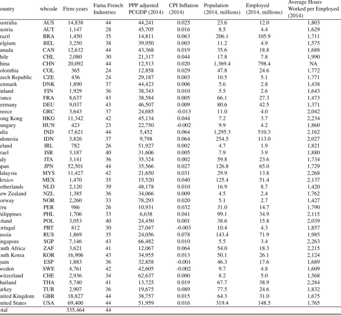
classification schemes, I repeat the exercise using the 2-digit SIC (Standard Industry Classifica-tion) codes. After these exclusions, the main analysis uses 334,608 firm-years across 42 countries. Table 1 provides summary statistics for the raw data.
Table 1 shows that there is a large variation in the sample size across countries. The US has the largest sample size with 69,400 firm-years, closely followed by Japan with 52,501 firm-years. The sample size is the smallest for Colombia, which has only 365 firm-years. Industry diversity also differs across countries; all 44 Fama-French (FF) industries are observed in Australia, China, Canada, India, United Kingdom and the United States. On the other hand, only 23 FF industries are observed in Hungary. Purchasing power parity (PPP) adjusted real GDP15, population, employ-ment, and average hours worked per employed are from the Penn World Tables 9.0. As data on average hours worked is not available for China, I use GDP per capita as the baseline measure of output per unit labor in this paper; I later check the robustness of the result using the GDP per hour worked and find that the result remain unchanged. Consumer price indices are from the World Bank database.
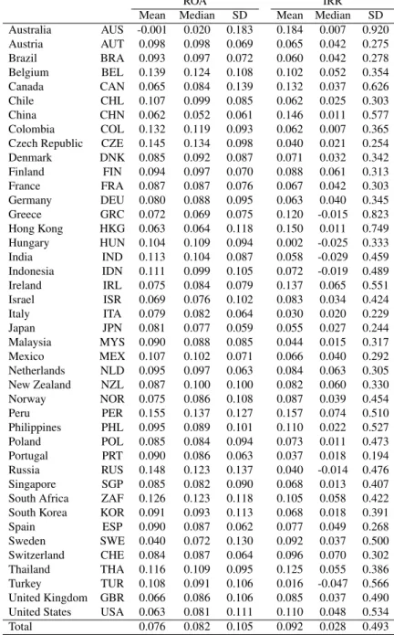
Table 2 provides summary statistics for the return on assets (ROA) and internal rate of return (IRR) estimates across countries. The data show two idiosyncrasies. First, the mean ROA for Australia is negative during the analysis period (1997-2014). This is due to the significant under-performance of the metal mining industry during and after the financial crisis, and excluding the metal mining companies (SIC 2-digit code: 10), Australia’s mean ROA turns positive.
Second, across the MSCI developed and emerging countries the average IRR is greater than the average ROA, a finding which seems at odds with the implications of the standard model (r = M P K −δ). The mean IRR across MSCI developed and emerging countries between 1997 and 2014 is9.2% and the mean ROA is7.6%. However, upon further examination this pattern is due to a large rightward skewness in the distribution of IRR, illustrated in Figure 1. The graph shows that compared to the ROA distribution (Figure 1a), which is almost perfectly symmetric across the mean, the IRR distribution (Figure 1b) is skewed to the right.
This pattern is also seen in the difference between the means and the medians in Table 2. The mean and the median ROA almost perfectly align with each other with a less than1% difference between the two values. On the other hand, the mean and the median IRR differ by6.4%! Due to the right skewness, even when the mean IRR is higher than the mean ROA, the median IRR is substantially lower than the median ROA. Thus, in the following section, I analyze not only the average cross-country patterns, but also the median trend across countries, to check for the effects of the skewness. The IRR is also substantially more volatile relative to ROA. The aggregate standard deviation for the ROA is10%, but it is49%for the IRR.
Figure 2 shows the two-way scatter plot between the median firm level ROA and IRR against the mean log(PCGDP) between 1997 and 2014. The figure also include the best fit line for the mean trend. Figure 2a is the two-way plot for the median ROA and the mean log(PCGDP); it shows a clear negative correlation between the two variables and a steep downward sloping best-fit line. On the other hand, the figure 2b, which is the two-way plot for the median IRR and the mean log(PCGDP), shows a positive correlation between the two variables and an upward sloping best-fit line suggesting a potential deviation between the cross-country marginal product of capital and the financial return patterns. While this positive financial return trend contradicts the predictions of the neoclassical model, it is consistent with the international capital flow pattern documented in Prasad, et al (2007). In the paper, they show that ”the relative income of [current account] surplus countries has fallen below that of deficit countries. Not only is capital not flowing from rich to poor countries, in quantities the neoclassical model would predict–a paradox pointed out by Lucas (1990)– but, in the last few years it has been flowing from poor to rich countries”.
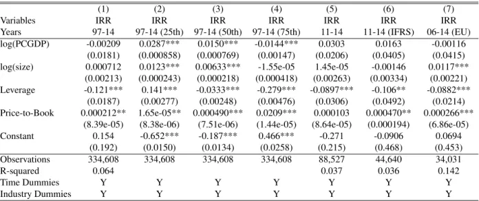
1.4 Cross Country Marginal Products of Capital and Investment Return Patterns
The standard neoclassical model predicts that both firm-level marginal product of capital and investment return will correlate negatively with per capital GDP. In this section, I conduct empirical analysis to test the implications of the standard model using firm-level data.
1.4.1 Firm-Level Return on Assets and Per Capita GDP
To formally assess the relationship between aggregate output per unit labor and the firm level profitability (return on assets), I estimate the following benchmark specification:
M P Kc,t,i,f =α+β1log(P CGDPc,t) +β2Dt+β3Fi+γXc,t,i,f +c,t,i,f (1.13)
M P Kc,t,i,f is the return on assets (ROA) for a firm f in industry i in country c in period t, and
P CGDPc,t is the purchasing power parity adjusted real per capita GDP in country c in period t
in 2011 US dollars that I use as a proxy for output per unit labor. Dt and Fi are time and
in-dustry dummies that are added to control for global macroeconomic shocks that occurred during the period of analysis, or an industry specific trend. Xc,t,i,f is the vector of firm specific factors, which includes the log size (the book value of assets denominated in USD; the value is adjusted for the inflation using the CPI index), leverage (book debt to equity ratio), and the equity price-to-book ratio. This vector adjusts for firm-specific risk, which are absent in the standard model. This vector of firm specific factors is motivated by Fama and French (1992); in the paper authors write that “if assets are priced rationally, our results suggest that stock risks are multidimensional. One dimension of risk is proxied by size, ME. Another dimension of risk is proxied by BE/ME, the ratio of the book value of common equity to its market value.” Leverage is added for com-pleteness although the effect of leverage on the return is debated in the literature.16 Note that the riskiness of the firm is expected to rise with a decrease in size and an increase in leverage and the price to book ratio. Errors are clustered in country-year to control for the firm-level error corre-lation within the country-year groups. As stated in their heavily cited paper, Cameron and Miller
(2015) write, “[f]ailure to control for within-cluster error correlation can lead to very misleadingly small standard errors, and consequent misleadingly narrow confidence intervals, large t-statistics and low p-values.” Therefore clustering of errors should enhance the precision of the coefficient estimates.17
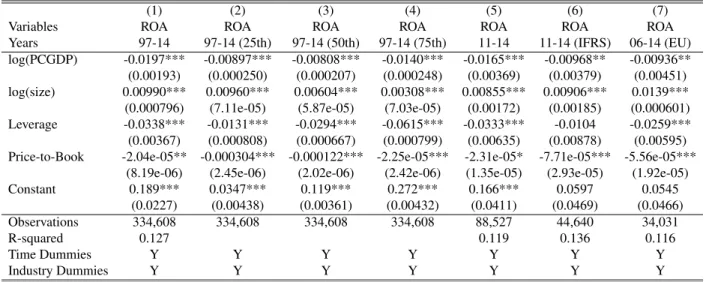
I do not include the country fixed effect in the benchmark regression due to the relatively moderate time dimension of the dataset (less than 20 years). Although country fixed effect is an attractive way to control for unobserved non-time varying country characteristics, “[i]nclusion of country fixed effects also affects the estimated coefficients of explanatory variables... Coefficients on country variables that are constant (such as geographical features and colonial history) cannot be estimated at all, and variables that have little within-country time variation cannot be estimated with precision.”(Barro, 2012). Considering the relatively small change in PPP adjusted PCGDP in 1997-2014 period especially among developed countries, the bias from the inclusion of country fixed effect is unlikely to be negligible. However, in appendix I do present the regression result with country fixed effect for periods 1997-2014 for robustness, and I find that the main result remain unchanged.18
Table 3 reports the results from the regression model. Column (1) shows the results for the MSCI developed and emerging countries between 1997 and 2014. Size has a statistically signifi-cant positive effect on the return on assets, and the price to book ratio and leverage have a negative and significant effect confirming the prediction that firm-level ROA rises with the increase in the firm specific risk. The statistically significant negative relationship between per capital GDP and the firm ROA shows that the implication of the standard neoclassical model holds during the period across firms in MSCI developed and emerging countries and controlling for the firm, industry, and time specific effects. In other words, as the model predicts the firm ROA falls with increases in the
17The errors are clustered by country-year rather than country due to limited number of country clusters. Camerona
and Miler (2015) state “we note that there is no specific point at which we need to worry about few clusters. Instead, ‘more is better’. Current consensus appears to be thatG= 50is enough for state-year panel data.” The authors also add that more clusters are needed in case of the unbalanced panel. Since the maximum possible number of country cluster is 42, which is arguably too few even for the balanced panel, I use country-year cluster for the main analysis. Regression result with country clusters however, are also presented in the appendix and the findings of the paper do remain robust.
proxy for labor productivity. This finding also suggests that if, on average, the first order condi-tion that equates the marginal product of capital and the investment return holds, then investment returns should also be inversely correlated with per capita GDP.
Column (1) shows that, on average, the firm-level ROA declines with increases in per capita GDP, but does not provide any insight on how the pattern differs within the sample. For example, what is the relationship between firm ROA and per capita GDP when we examine high productivity firms with an above average return on assets. Quantile regressions make up for this shortcoming of the OLS regression by modeling the relationship between the specified percentile of the response variable and the control variables, i.e., the median quantile regression portrays the relationship between the median marginal product of capital and the predictor variables, etc. For a more com-prehensive analysis, I run a quantile regression for the 25th, 50th (median), and the 75th percentile firms. Also note that this question is particularly important in analyzing the differences between internal rates of return (IRR) and the return on assets, due to the high level of skewness observed in the distribution of the internal rates of return in Table 2.
Columns (2) −(4) show that the coefficient on per capita GDP is consistently statistically significant across the 25th, 50th, and the 75th percentiles. The negative slope is the steepest for the firms in the 75th percentile of ROA, and there is a little difference in the slope between the 25th and the 50th percentile. The finding suggests that the effect of the changes in the aggregate output per unit labor is most acutely felt by the ”most productive” firms in the economy.
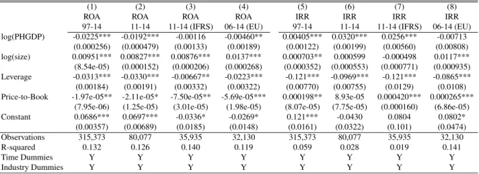
As the data section mentions, the period of analysis includes the global financial crisis, during which financial systems went through substantial stresses.19 Therefore, I repeat the exercise in column (1) for the 2011-2014 post-financial crisis period. Due to the short period of analysis, the values are susceptible to skewness from the market volatility, but the regression results presented in column (5) confirm the findings in column (1). Columns (6) and (7) check for the effect of the cross-country differences in the accounting standards. Column (6) repeats the regression in column (5) using firms from the countries that adopted the International Financial Reporting Standards
(IFRS) during the post-financial crisis period, and the column (7) shows the results using firms in MSCI EU countries during 2006-2014– the European Union officially adopted IFRS starting 2005.20 This result is particularly insightful as the area enjoys a relative low capital flow barriers across countries within the Eurozone21 which is consistent with the free-capital flow assumption within the standard neoclassical model. The results presented in columns (5)-(7) of Table 3 show that the inverse correlation between per capita GDP and firm-level ROA is surprisingly consistent across time, and is robust to cross-country differences in accounting standards.
Table 4 examines the relationship between ROA and per capita GDP with industry-level con-trols. I estimate the following industry by industry regression for each of the 48-Fama French industry (44 excluding financial industries) using the base sample of firms in the MSCI developed and emerging countries between 1997 and 2014. Table 4 presents the results.:
M P Kc,t,f =α+β1log(P CGDPc,t) +β2Dt+γXc,t,f +c,t,f (1.14)
Table 4 confirms that the cross-country pattern observed in the Table 3 is not industry-specific. Firm ROAs decline with increases in per capita GDP in almost all 44 non-financial Fama-French industries. Thirty six industries have statistically significant negative coefficients for per capita GDP, and only one industry (aircraft manufacturing) has a statistically significant positive coeffi-cient. The negative coefficient is steepest in the medical and the defense industries, which require high-levels of human capital. The Appendix presents a similar analysis using SIC 2-digit indus-tries and the results remain unchanged. A majority of indusindus-tries have a statistically significant negative coefficient for per capita GDP, and only a few industries have an insignificant or positive coefficient.
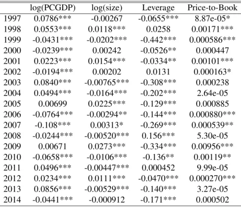
Table 5 further shows that the observed results are not time-specific. It shows the results for
20see Guggiola (2010)
21“In the EUs single market (sometimes also called the internal market) people , goods , services , and money can
the following estimating equation using the base sample:
M P Kc,i,f =α+β1log(P CGDPc) +β2Fi+γXc,i,f +c,i,f (1.15)
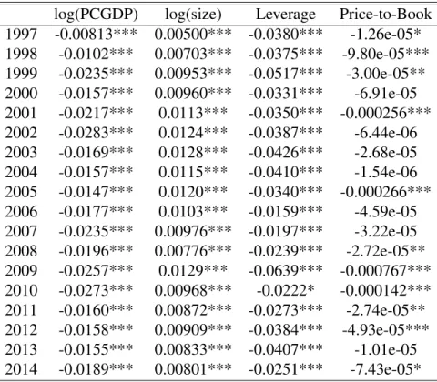
Between 1997 and 2014, we observe a statistically significant negative coefficient for all years. The coefficient is most negative during the financial crisis (2007 and 2009). The negative coeffi-cient slowly flattens post-2010, as the developed countries recover. Conversely, the negative slope is relatively flat during the Asian Financial Crisis (1998) and slowly steepens as the Asian tigers move out of their deep recessions.
The results presented in this section show that consistent with the neoclassical model, the marginal product of capital is higher in countries with low per capita GDP. In the following sub-section, I repeat the exercises using the investment return (IRR).
1.4.2 Investment Returns and Per Capita GDP
In order to test for the validity of the firm first order condition described in equation (6), I use the following regression specification:
rc,t,i,f =α+β1log(P CGDPc,t) +β2Dt+β3Fi+γXc,t,i,f +c,t,i,f (1.16)
The predictor variables in the equation are identical to those in equation (13), but the dependent variable is now the internal rate of return (IRRc,t,i,f). As in the equation (13), firm-level factors
such as size, leverage, and the price to book ratio control for the firm-specific characteristics, and industry and time dummies control for industry and time specific effects. Errors are also clustered in country-year groups as in the previous subsection. If the standard relationship between the firm investment return and marginal product of capital holds, then the internal rate of return should also be inversely correlated with per capita GDP.
GDP is not statistically significant when one controls for firm and industry specific factors. This result implies that the cross-country marginal product of capital and investment return patterns do not necessarily mirror each other– as the neoclassical model predicts. This finding questions the validity of the standard approach which uses aggregate marginal product of capital to explain the pattern of international capital flows. The finding also suggests that even accurate measures of marginals product of capital may not explain patterns of international capital flows as the marginal product of capital may be an inaccurate proxy for investment returns.
The finding therefore suggests that “there is no prima facie support for the view that interna-tional credit frictions play a major role in preventing capital flows from rich to poor countries.” (Caselli and Feyrer, 2007). As Lucas suggests, if investment returns are inversely correlated with per capita GDP, capital ought to flow rapidly from developed to emerging market countries and any deficiencies in these flows imply international financial market frictions. However, the results in Column (1) suggest that the investment returns are relatively equal across developed and emerging countries and therefore there may not be an incentive for the capital to flow to the emerging mar-kets since opportunities with similar investment returns also exist within developed economies. This empirical evidence does not appear consistent with the claim that international investment barriers play a major role in explaining the lack of capital flow to emerging countries. A potential resolution to the Lucas paradox may therefore lie in the cross-firm or cross-industry variation in internal rates of return within countries.
to higher investment returns, this is not necessarily true for the less-productive firms in the coun-try. One should also note that the counter-intuitive positive coefficient is steeper for the bottom 25th percentile versus the median. This strengthens the argument by Banerjee and Duflo (2005) which suggests that the key to Lucas Paradox may not lie so much with ‘international’ factors, but ‘domestic’ factors.
Column (5) presents the results for the post-financial crisis period and reaffirms the divergence between the marginal product of capital and the investment return patterns observed in column (1). The coefficient on P CGDP is positive and statistically significant, which implies that the investment return in developed countries is in fact higher than that in emerging countries during the sample period. Column (6) repeats the regression in column (5) using only the firms that adopted IFRS accounting standards during the period, and documents that the cross-country pattern observed in column (5) is robust to cross-country differences in the accounting standards. Column (7) also repeats the exercise in column (1) using the MSCI EU countries that share the streamlined IFRS accounting standard since 2005 and finds thatP CGDP is statistically insignificant.
Table 7 shows the results for the following specification to check for any variation in cross-country IRR patterns across industries:
rc,t,f =α+β1log(P CGDPc,t) +β2Dt+γXc,t,f +c,t,f (1.17)
The results confirm the aggregate pattern observed in Table 6. The coefficient on per capita GDP is statistically insignificant or positive and significant in 35 out of 44 industries. Only nine industries have a statistically significant negative coefficient, and the slope is barely significant at the 10%
level in the four among the nine industries. This result contrasts sharply with Table 4, in which 36 industries have a statistically significant negative coefficient. It further confirms the finding that the cross-country marginal product of capital pattern does not appear to match the investment return pattern.
annual variation in the cross-country internal rate of return pattern:
rc,i,f =α+β1log(P CGDPc) +β2Fi+γXc,i,f +c,i,f (1.18)
Between 1997 and 2014, the coefficient on P CGDP is statistically insignificant or positively significant for 10 years. The negatively significant coefficient is observed for eight years, and four of the eight years occur around the financial crisis (2006-2008, and 2010). The negative slope is also the steepest during this period (2006 and 2010). The finding again confirms that the inverse correlation between the marginal product of capital and per capita GDP does not necessarily translate to an inverse correlation with investment returns as the neoclassical model predicts.
The empirical result in this section documents a divergence between the cross-country invest-ment return and the marginal product of capital patterns, and show that this finding is surprisingly robust across different sets of countries and time periods. This result questions the validity of the traditional approach which uses marginal product of capital to explain the international capital flow patterns, and further suggests that the standard link between marginal product of capital and the fi-nancial return does not hold in a sample of developed and emerging countries between 1997-2014. As this standard link between the two variables stems from the frictionless capital accumulation equation, this empirical finding highlights the importance of cross-country capital efficiency (i.e. the level of future capital input that can be obtained from a unit investment today) difference in explaining the Lucas Paradox.
In the following subsection, I check the effect of cross-country difference in the employment and taxes, to further confirm the robustness of the result documented thus far.
1.5 Additional Test and Robustness Checks
1.5.1 Robustness Check: Hourly labor input
In the previous two subsections, I use per capita GDP as the measure of output per unit labor. While this is a widely used measure of economic performance22, in this subsection, I check the robustness of the results using output per hours worked.
Output per hours worked is estimated using the following equation:
P HGDPc,t =
GDPc,t
AHWc,t∗Empc,t
(1.19)
AHWc,t is the average annual hours worked by person employed, and Empc,t is the employed
population in countryc, in timet. P HGDPc,t is a commonly used measure of labor productivity
in the macroeconomics literature23 and is more precise measure of the output per unit labor input relative toP CGDPc,t, as it measures the labor input by hour. Another commonly used measure of
productivity is GDP per person employed. However, this ratio tend to over-estimate the productiv-ity of workers in emerging countries as it fails to account for the longer working hours in emerging countries. Even in 2014, the average annual hours worked by person employed in Thailand was almost 1.7 times that in Germany. Therefore, ignoring cross-country differences in the average hours worked can bias the results over-estimating the labor efficiency of the workers in emerging countries. One drawback of the output per hours worked measure is that China has to be dropped from the sample due to a lack of data. However, the regression result using the 315,373 firm-years across 41 countries should still provide a reliable estimate of the cross-country return patterns.
To check the robustness of the results presented in sections 4.1 and 4.2, I use the following equations, which replacelog(P CGDPc,t)withlog(P HGDPc,t):
M P Kc,t,i,f =α+β1log(P HGDPc,t) +β2Dt+β3Fi+γXc,t,i,f +c,t,i,f (1.13’)
22see Caselli and Feyrer (2007), Banerjee and Duflo (2005), Gourinchas and Jeanne(2009)
rc,t,i,f =α+β1log(P HGDPc,t) +β2Dt+β3Fi+γXc,t,i,f +c,t,i,f (1.16’)
Table 9 presents the results. Columns (1)-(4) reports results for the equation (13’), and columns (5)-(8) report results for equation (16’). The columns (1)-(4) show that the findings about the marginal product of capital from section 4.1 remain robust. The coefficient on per capita GDP is negative and significant for the base sample excluding China (Column 1), post-financial crisis period (Column 2), and in Euro-zone post-2005 (Column 4). The coefficient on per capita GDP is statistically insignificant for post-financial crisis period IFRS countries (Column 3), which may be due to the small sample size. Columns (5)-(8) further highlight the findings on internal rates of return in section 4.2. The coefficient on per capita GDP is positive and significant for the base sample excluding China (Column 5), post-financial crisis period (Column 6), and post-financial crisis period IFRS countries (Column 7). Per capita GDP has a statistically insignificant impact on internal rates of return in Euro-zone countries post-2005 (Column 8).
The empirical results presented in this section confirm the findings of section 4.1 and 4.2, and questions the validity of the standard approach which use marginal product of capital to explain the international capital flow.
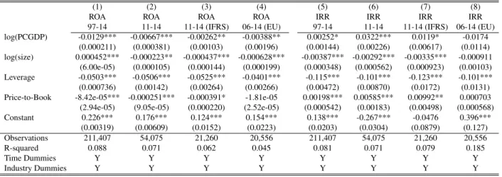
1.5.2 Robustness Check: Tax adjusted income
In the previous two sections, I use EBITDA as a measure of the capital owner’s earnings to calibrate firm ROAs and investment returns. Although EBITDA is a consistent with the standard model, it does not take into account government taxes, which reduce the actual income received by the capital holders. Therefore, in this section, I check the robustness of the main results using the following tax-adjusted estimates of MPK and the investment return, following the example of Fama and French (1999)24:
24I do note that this is not the most accurate measure of the tax-adjustment due to deferred taxes within most firms,
ROAc,t,i,f =
EBIT DAc,t,i,f(1−trc,t,i,f)
(M V Ac,t−1,i,f)(1+inf lc,t) (1.20)
IRRc,t,i,f =
EBIT DAc,t,i,f(1−trc,t,i,f)+[−adj∆Assetc,t,i,f+M V Ac,t,i,f−M V Ac,t−1,i,f]
M V Ac,t−1,i,f −inf lc,t (1.21)
trc,t,i,f is the income tax rate on firmf, in industry i in time t, in country c. An alternative
expression for tax-adjusted income is EBIT DAc,t,i,f −T axc,t,i,f, where T axc,t,i,f is the actual
income tax on firmf. However,EBIT DAc,t,i,f(1−trc,t,i,f)should provide a tax-adjusted income
estimate that is more consistent with the model, as the amount of tax imposed on the firm is based on the income after deduction of interest income and expense. Therefore,EBIT DAc,t,i,f−
T axc,t,i,f, where T axc,t,i,f is the actual income tax on firm f, and should lead to large variation
on the post-tax income based on the capital structure of the specific firm. On the other hand, the estimate based on the tax rate is less affected by the capital structure of the firm, reducing potential bias from the capital structure differences across the firms.
The tax-adjusted measures of ROAand IRR reduce the size of the sample, as they exclude firm-years without tax-rate data. Therefore, the cross-country pattern is estimated using 211,407 firm-years across 42 countries, rather than 315,373 firm-years. Table 10 presrnts the empirical results from equations (13) and (16), using the tax-adjustedROAandIRR. Columns (1)-(4) re-port the results from the equation (13), and columns (5)-(8) rere-port the results from the equation (16). Columns (1)-(4) confirm the original finding thatlog(P CGDPc,t)and the marginal product
of capital are inversely correlated. The coefficient forlog(P CGDPc,t)is significantly negative in
the base sample (Column 1), post-financial crisis period (Column 2), IFRS countries post financial period (Column 3), and Euro-zone countries post 2006 (Column 4). On the other hand, column (5) shows that thelog(P CGDPc,t)is a positive and significant predictor ofIRRin the base
crisis period.log(P CGDPc,t)is statistically insignificant in Euro-zone countries post-2006.
These finding shows that the empirical result documented in sections 4.1 and 4.2 are extremely robust across different specifications and samples. There seems to be a non-negligible gap between the cross-country marginal product of capital pattern and the investment return pattern, which suggests that the question ”why the capital doesn’t flow to emerging countries?” is intricately tied to this gap between the two variables. Based on this finding, in the following section I propose a modification to the traditional neoclassical model, which can potentially model the gap between marginal product of capital and investment return documented in this section. I also investigate alternative macroeconomic variables often used in the Lucas Paradox literature, to find the factors that can potentially affect the size of the observed gap between the marginal product of capital and the investment return.
1.6 Conclusion
According to the textbook neoclassical theory, if two countries share the identical production function, and the trade in capital good is free and competitive, new investment will only occur in the poorer country since the marginal return to capital should be higher in economies with less capital (due to the law of diminishing return). However, as Lucas pointed out in his seminal paper in 1990, observed capital flow from developed to developing countries fall short of what should be observed according to the theory. This phenomena has been named ”Lucas Paradox” and has been one of the major puzzles in the macroeconomic literature.
despite the international difference in marginal product of capital. This finding also suggests that the key issues in explaining the international capital flow is not an ”international” credit frictions but rather a ”domestic” credit frictions which affects the capital accumulation process. Thus, the future research on Lucas Paradox should focus not only on factors that affect productive efficiency, but also those that affect the capital efficiency.
Table 1.1: Data Summary Statistics (1997-2014)
The sample includes all non-financial (all SIC codes except 6000∼6999) balance sheet solvent firm-years in the Worldscope database with 1) market value(WC08001), assets(WC02999), liabilities(WC03351), depreciation(WC01151), EBITDA(WC18198), extraordinary credit(WC01253) and extraordinary charge(WC01254) data for the year and; 2) debt and market value data for the previous year in the MSCI developed and emerging countries (excluding Saudi Arabia, Qatar and UAE) between 1997 and 2014. Purchasing Power Parity (PPP) adjusted per capita GDP (PCGDP) is calibrated using the PPP adjusted GDP(rgdpo) and the population (pop) estimate from the Penn World Table 9.0. Employed population (emp), and average hours worked per employed (avh) are also from the Penn World Table 9.0. CPI inflation is from the World Bank
Country wbcode Firm-years Fama French Industries PPP adjusted PCGDP (2014) CPI Inflation (2014) Population (2014, millions) Employed (2014, millions) Average Hours Worked per Employed (2014)
Australia AUS 14,838 44 44,241 0.025 23.6 12.0 1,803
Austria AUT 1,147 28 45,705 0.016 8.5 4.4 1,629
Brazil BRA 1,450 35 14,811 0.063 206.1 105.9 1,711
Belgium BEL 3,250 38 39,950 0.003 11.2 4.9 1,575
Canada CAN 12,632 44 43,368 0.019 35.6 18.8 1,688
Chile CHL 2,080 30 21,317 0.044 17.8 7.8 1,990
China CHN 20,092 44 12,513 0.020 1,369.4 798.4 NA
Colombia COL 365 24 12,858 0.029 47.8 24.6 1,772
Czech Republic CZE 436 24 29,187 0.003 10.5 5.1 1,771
Denmark DNK 1,890 37 44,423 0.006 5.6 2.8 1,438
Finland FIN 1,929 36 38,343 0.010 5.5 2.6 1,643
France FRA 8,637 43 38,584 0.005 66.1 27.3 1,473
Germany DEU 9,037 43 46,507 0.009 80.6 42.5 1,371
Greece GRC 3,643 37 24,685 -0.013 11.0 4.0 2,042
Hong Kong HKG 11,342 42 45,134 0.044 7.2 3.7 2,234
Hungary HUN 423 23 22,750 -0.002 9.9 4.2 1,860
India IND 17,621 44 5,452 0.064 1,295.3 510.3 2,162
Indonesia IDN 3,826 37 9,798 0.064 254.5 113.0 2,027
Ireland IRL 782 26 51,927 0.002 4.7 1.9 1,821
Israel ISR 3,187 40 31,606 0.005 7.9 3.9 1,880
Italy ITA 3,141 36 35,324 0.002 59.8 23.6 1,734
Japan JPN 52,501 44 35,566 0.027 126.8 65.0 1,729
Malaysia MYS 11,427 42 21,650 0.031 29.9 13.8 2,268
Mexico MEX 1,470 35 15,520 0.040 125.4 51.4 2,137
Netherlands NLD 2,120 39 48,178 0.010 16.9 8.7 1,420
New Zealand NZL 1,385 36 34,066 0.009 4.5 2.4 1,762
Norway NOR 2,260 33 78,293 0.020 5.1 2.7 1,427
Peru PER 986 26 10,931 0.032 31.0 14.7 1,790
Philippines PHL 1,706 33 6,638 0.041 99.1 34.9 2,115
Poland POL 3,053 40 24,450 0.001 38.6 15.8 2,039
Portugal PRT 812 30 27,047 -0.003 10.4 4.3 1,857
Russia RUS 1,869 35 24,056 0.078 143.4 71.9 1,985
Singapore SGP 7,146 43 66,482 0.010 5.5 3.4 2,263
South Africa ZAF 3,621 41 12,067 0.064 54.0 18.3 2,215 South Korea KOR 16,906 43 34,955 0.013 50.1 26.1 2,124
Spain ESP 1,883 36 32,858 -0.001 46.3 17.6 1,689
Sweden SWE 4,761 42 42,605 -0.002 9.7 4.8 1,609
Switzerland CHE 2,936 34 62,637 0.000 8.2 5.0 1,568
Thailand THA 5,740 41 13,725 0.019 67.7 38.9 2,284
Turkey TUR 2,907 36 19,675 0.089 77.5 24.6 1,832
United Kingdom GBR 18,827 44 38,757 0.015 64.3 31.0 1,675 United States USA 69,400 44 51,959 0.016 319.4 148.5 1,765
Table 1.2: Summary Statistics: ROA vs. IRR (1997-2014)
ROAc,t,i,f =
EBIT DAc,t,i,f
(P Vc,t1,i,f)(1 +inf lc,t)
IRRc,t,i,f =
EBIT DAc,t,i,f+ [−Adj∆Assetc,t,i,f+P Vc,t,i,f−P Vc,t−1,i,f]
P Vc,t−1,i,f
−inf lc,t
ROAc,t,i,fis the ratio between the firm EBITDA before extraordinary items (sum of EBITDA after extraordinary items (WC18198) and extraordinary cost (WC01254) minus extraordinary credit(WC01253)) and the market value of asset (sum of market value of equity(WC08001)and the book value of liabilities(WC03351)) from the previous year adjusted for CPI inflation.IRRc,t,i,fis the ratio between the sum of EBITDA before extraordinary item, change in the market value of asset less the change in the book value of asset and the market value of asset from the previous year adjusted for CPI inflation
ROA IRR
Table 1.3: MSCI Developed and Emerging Countries: Firm ROA and PCGDP Purchasing Power Parity (PPP) adjusted per capita GDP (PCGDP) is calibrated using the PPP adjusted GDP(rgdpo) and the population (pop) estimate from the Penn World Table 9.0. Size is the inflation adjusted book value of the firm’s asset in US dollar, and leverage is the ratio between the book value of liability and the assets. Price-to-Book measures the ratio between the market and the book value of the firm equity. Time dummies and industry dummies for the 48 Fama-French Industries are included in all regressions. Standard deviation is reported in the parenthesis.
(1) (2) (3) (4) (5) (6) (7) Variables ROA ROA ROA ROA ROA ROA ROA Years 97-14 97-14 (25th) 97-14 (50th) 97-14 (75th) 11-14 11-14 (IFRS) 06-14 (EU) log(PCGDP) -0.0197*** -0.00897*** -0.00808*** -0.0140*** -0.0165*** -0.00968** -0.00936** (0.00193) (0.000250) (0.000207) (0.000248) (0.00369) (0.00379) (0.00451) log(size) 0.00990*** 0.00960*** 0.00604*** 0.00308*** 0.00855*** 0.00906*** 0.0139*** (0.000796) (7.11e-05) (5.87e-05) (7.03e-05) (0.00172) (0.00185) (0.000601) Leverage -0.0338*** -0.0131*** -0.0294*** -0.0615*** -0.0333*** -0.0104 -0.0259*** (0.00367) (0.000808) (0.000667) (0.000799) (0.00635) (0.00878) (0.00595) Price-to-Book -2.04e-05** -0.000304*** -0.000122*** -2.25e-05*** -2.31e-05* -7.71e-05*** -5.56e-05***
(8.19e-06) (2.45e-06) (2.02e-06) (2.42e-06) (1.35e-05) (2.93e-05) (1.92e-05) Constant 0.189*** 0.0347*** 0.119*** 0.272*** 0.166*** 0.0597 0.0545
(0.0227) (0.00438) (0.00361) (0.00432) (0.0411) (0.0469) (0.0466) Observations 334,608 334,608 334,608 334,608 88,527 44,640 34,031 R-squared 0.127 0.119 0.136 0.116 Time Dummies Y Y Y Y Y Y Y Industry Dummies Y Y Y Y Y Y Y