HYDROGEN BURNING OF THE RARE OXYGEN ISOTOPES
Matthew Quinn Buckner
A dissertation submitted to the faculty at the University of North Carolina at Chapel Hill in partial fulfillment of the requirements for the degree of Doctor of Philosophy in the Department of Physics.
Chapel Hill 2014
Approved by: Christian Iliadis Gerald Cecil
c
⃝2014
ABSTRACT
Matthew Quinn Buckner: HYDROGEN BURNING OF THE RARE OXYGEN ISOTOPES (Under the direction of Christian Iliadis)
At the Laboratory for Experimental Nuclear Astrophysics (LENA), two rare oxygen isotope proton cap-ture studies were performed at low energies—18O(p,γ)19F and17O(p,γ)18F. The goal of each study was to
improve thermonuclear reaction rates at stellar plasma temperatures relevant to18O and 17O destruction,
respectively. The stellar nucleosynthesis temperature regime corresponds to very low proton bombarding energies. At these low energies, the Coulomb barrier suppresses the reaction yield in the laboratory, and environmental backgrounds dominate the detected signal, making it difficult to differentiate the γ-cascade from background. At LENA, the electron cyclotron resonance (ECR) ion source produces intense, low-energy proton beam, and these high currents boost the reaction yield. LENA, a “sea-level” facility dedicated to nuclear astrophysics, also has a coincidence detector setup that reduces environmental background contribu-tions and boosts signal-to-noise. The sensitivity afforded by γγ-coincidence and high beam current allowed these rare oxygen isotope reactions to be probed at energies that correspond to stellar plasma temperatures. For stars with masses between 0.8 M⊙ ≤M≤8.0 M⊙, nucleosynthesis enters its final phase during the asymptotic giant branch (AGB) stage. This is an evolutionary period characterized by grain condensation that occurs in the stellar atmosphere; the star also experiences significant mass loss during this period of instability. Presolar grain production can often be attributed to this unique stellar environment. A subset of presolar oxide grains features dramatic18O depletion that can not be explained by the standard asymptotic
giant star burning stages and dredge-up models. An extra mixing process for low-mass asymptotic giant branch stars, known ascool bottom processing (CBP), was used in the literature to explain this and other anomalies. Cool bottom processing can also occur during the red giant branch (RGB) phase, but it is not thought to contribute to the extreme 18O depletion observed within certain stellar environments and
within presolar grain samples. However, intense depletion could result from the 18O +pprocesses during
cool bottom processing in low-mass AGB stars. A portion of this dissertation describes a study of the
18O(p,γ)19F reaction at low energies performed at LENA. Based on these new results, it was found that the
resonance at ER = 95 keV has a negligible effect on the reaction rate at the temperatures associated with
of this research is a new thermonuclear reaction rate for18O(p,γ)19F. These results were published in Buckner et al. (2012) [1].
Classical novae are thought to be among the dominant sources of 17O in the Galaxy. These energetic
events produce18F that, as it decays to18O, emits positrons that annihilate with electrons producing 511
keVγ-rays. These emissions occur at timescales that correspond to a transparent nova expansion envelope making their observation possible and important for constraining nova stellar models. The importance of the non-resonant component of the17O(p,γ)18F reaction is well established, and numerous studies have been
performed to analyze this reaction. The experimental tools available at LENA, in addition to a novel spectral analysis method, allowed the17O(p,γ)18F reaction to be studied within the classical nova Gamow window,
and new total S-factors were measured. The lowest energyin-beam17O(p,γ)18F measurement ever made was
collected during this experiment. A new direct capture S-factor was determined, and it was confirmed that this S-factor is constant at low energies. The ER= 193 and 518 keV resonances were also measured, and new
resonance strengths were determined. New 17O(p,γ)18F thermonuclear reaction rates are reported within
this thesis. The direct capture contribution, combined with updated partial widths and strengths from the literature, improved reaction rate uncertainties at low temperatures and may also impact17O overproduction
ACKNOWLEDGEMENTS
I do not think I can convey how truly grateful I am to Dr. Thomas Clegg for recognizing my potential, and during my first visit to the University of North Carolina at Chapel Hill, encouraging me to consider a generous offer from the Department of Physics and Astronomy. He also convinced me to work at the Laboratory for Experimental Nuclear Astrophysics (LENA) at Triangle Universities Nuclear Laboratory (TUNL). Tom and Dr. Christian Iliadis became my Master’s research advisors, and I began working on several different projects for them as I took classes my first year and studied for the written qualifying examination. Tom pushed me to apply for several fellowships, and I credit Tom for my successful application to the DOE NNSA Stewardship Science Graduate Fellowship. Additionally, Tom’s friendship with Dr. Jay Davis at Lawrence Livermore National Laboratory (LLNL) facilitated my placement at LLNL’s Center for Accelerator Mass Spectrometry (CAMS) during the summer of 2010. This summer practicum fulfilled the internship requirement stipulated by my DOE fellowship. Tom guided me during my first project at LENA, pulsing the electron cyclotron resonance (ECR) ion source proton beam and several other instrumentation projects. I love building and developing new hardware, and being able to work on a few instrumentation projects early in my graduate career helped me transition from my scholarly pursuits as an undergraduate to working in a laboratory environment as a graduate student.
When I started working with Christian in addition to Tom, my longterm research goals began to really take shape. My thesis advisor, Dr. Christian Iliadis, is a titan within the nuclear astrophysics community, and it is an honor and a privilege to work with him. His input, advice, criticism, and support were incredibly valuable throughout my graduate experience, and I am eternally indebted to him for his patience and his willingness to provide guidance. His expertise in detector setup, data acquisition electronics, and spectral analysis were invaluable, and I gained a significant amount of experience and understanding working alongside him as I developed my detector and DAQ configuration. He shared his indomitable wealth of knowledge and experience with regard to all aspects of my graduate endeavors, from theoretical calculations to experiment design to drafting peer reviewed papers. Christian was also extremely approachable and always eager to meet and discuss progress, setbacks, and anomalies over a cup of coffee; he was the quintessential thesis advisor and I can not thank him enough.
resources necessary for LENA to endure were always on hand. I recall numerous occasions where Art and I worked on conditioning the accelerators, and my familiarity with ion sorcery stems directly from these collaborations. Not only is Art a truly impressive experimentalist, he is also a gifted educator. Perhaps my fondest memory of graduate coursework at UNC was when Art took the reigns of a nuclear physics class and taught us material that would prove essential to my thesis work. I have also often relied on Art for his expert advice on technical and experimental issues, and I have him to thank for so many of the technical skills I have acquired.
Thank you to Dr. Fabian Heitsch and Dr. Gerald Cecil for their role as my dissertation committee members. I acknowledge the support of the US Department of Energy under Contract no. DE-FG02-97ER41041 and the DOE NNSA Stewardship Science Graduate Fellowship under Grant no. DE-FC52-08NA28752.
Aside from Professors Clegg, Iliadis, and Champagne, the one person who is most responsible for my evolution from undergraduate astrophysics scholar to a nuclear astrophysics doctoral candidate is Dr. John “Johnny” Cesaratto. When I first arrived at LENA, I found Johnny to be incredibly talented and intimi-dating. His focus, tenacity, and technical skills were both terrifying and awe-inspiring. However, I realized quickly that I could learn a lot from Johnny Cesaratto. I remember struggling to master conditioning the ECR ion source and tuning the accelerators under his tutelage. I am sure my persistent, naive questions were a constant frustration for him, but his calm, patient explanations of electronics, beam transport, signal processing, and ion sorcery were unequivocally critical to my progression, growth, and success as a graduate student. Johnny filled a void at LENA that became all the more apparent after his departure. I assert that if I even somewhat live up to his legacy and fill the vacuum he left behind at this laboratory, I do so because I learned from the best; I am the scientist I am today because of Johnny Cesaratto, and I can not think of a better role model and mentor.
of this experience, I advise every new graduate student that joins the LENA group to learn a programming language and to start exploring ROOT.
Dr. Stephen Daigle was always an excellent sounding board for theories and thought experiments. Whether it was refining a computational goal, tweaking the progression of an experiment, or pouring over a textbook to extract a key piece of information, Stephen was helpful, jovial, and amiable. Stephen and I spent a lot of time working together during the laboratory phase of his 14N(p,γ)15O experiment, and
that experience bolstered my technical skills, giving me the opportunity to refresh my accelerator operation technique. I appreciate everything Stephen did for me during my graduate career; he was always quick to offer advice or help when necessary.
The other post-doctoral fellow working at LENA, Dr. Anne Sallaska, also made a valuable contribu-tion to my overall development as a doctoral student. During her career, Anne gained computacontribu-tional and experimental experience, and endured and succeeded despite periodic setbacks and unexpected challenges. Because of her experiences as a graduate student and post-doc, I consider Anne extremely competent and even battle-hardened, and I value her opinion and critiques. I hope that if I am ever in her position, I can provide the quality constructive criticism and insights that I came to expect from her.
I believe that we only truly learn something when we are given the opportunity to teach it to someone else. Keegan Kelly proved that he is not only a brilliant and eager student, he was also incredibly helpful with everything from detector setup to data collection. His role as copilot during Stephen’s 14N(p,γ)15O
experiment and my 17O(p,γ)18F experiment was critical for Stephen and I to each proceed to graduation;
I am forever indebted to Keegan for his willingness to commit time and energy to these projects, and I am certain this process benefited his growth as an experimental physicist.
Dr. Richard Longland and Dr. Joseph Newton each contributed in small ways to my research by writing codes that I used or augmented, or by having important conceptual conversations with me.
TUNL technical staff members Jeff Addison, Bret Carlin, John Dunham, Patrick Mulkey, Richard O′Quinn, and Chris Westerfeldt were all extremely helpful, and I can not thank them enough for their contri-butions. I am particularly indebted to Bret for actively participating in brainstorming and troubleshooting sessions, and for making major contributions to my progression towards graduation.
During my experiment, Lori Downen was an excellent assistant and student. She was very helpful during the data acquisition phase of my17O(p,γ)18F experiment.
data acquisition.
Additionally, I would like to thank Grayson Rich for upgrading the ECRIS remote control system. This was truly a daunting project, but I had complete faith in Grayson’s incredible attention to detail and ability to design and to engineer complex control systems. The system he gave us is superb and I can not thank him enough.
The Duke University and UNC machine shops were also contributors to the realization and fabrication of key items critical to the completion of this research. Both shops contributed to the production of a new target box, anodization chamber, ECR ion source aluminum liner, and plasma chamber heat sink.
I can not thank all of these scholars, educators, and technicians without thanking that one educator who over a decade ago taught me the fundamental laws of Nature and encouraged me to pursue higher education in the sciences. Thank you, Mr. Frank Romano for challenging me, motivating me, and inspiring me to excel. Thank you for helping me discover that I could harness both my intellect and my creativity, and simultaneously wield them to uncover the mysteries of the Universe and peer into the depths of cosmic cauldrons.
Also, a special thanks to visionary artist, and my good friend, Mr. John Cheer. John, you unwittingly provided me with my first “laboratory” experience and fodder for all of those graduate school essays. Thank you for your friendship and the steady income during college.
I would like to thank my friend Jennifer White for not only agreeing to proofread this dissertation, but for actually reading through the entire document (twice) and supplying me with grammatical corrections. I can not think of many people I know who would agree to review my thesis, put in the time and effort to actually follow through, and provide valuable feedback. Thank you, Jenn.
Mom and Dad, throughout my life you were my loudest supporters, and I know that I won your love and affection on day one. I know I did not need to get a doctoral degree to make you proud of me, but I went ahead and did it anyway. Thank you both for giving Ben and me everything you had. Thank you for answering all of my questions as a child, for telling me stories, for reading to me, for taking me on walks behind Rockledge looking for whales, for teaching me so much, and for nurturing both the profoundly creative and intensely quizzical sides of my personality. I love you both so much. Thank you.
Benjamin, thank you for always believing in me and encouraging me. You are an amazing brother and one of my best friends; the relationship we are able to have as adults seems to be rare among siblings. You never cease to amaze me and serve as a reminder to flex my own creativity and imagination.
TABLE OF CONTENTS
LIST OF TABLES . . . xv
LIST OF FIGURES . . . .xvii
1 INTRODUCTION . . . 1
1.1 Astrophysical Motivation . . . 1
1.1.1 Cool Bottom Processing in Low-Mass AGB Stars . . . 2
1.1.2 Explosive Hydrogen Burning During Classical Novae . . . 6
1.2 Focus . . . 11
2 NUCLEAR ASTROPHYSICS THEORY . . . 12
2.1 Thermonuclear Reaction Rates . . . 12
2.1.1 Non-Resonant Reaction Rates . . . 13
2.1.2 Resonant Reaction Rates . . . 18
2.2 Monte Carlo Reaction Rates . . . 21
2.2.1 Probability Density Functions . . . 22
3 ACCELERATORS AND DETECTORS . . . 24
3.1 The Accelerators . . . 26
3.1.1 1 MV JN Van de Graaff . . . 26
3.1.2 ECR Ion Source . . . 27
3.2 New Beam Rastering System . . . 32
3.3 Preliminary Investigation into Beam Pulsing . . . 33
3.4 Target Chamber . . . 35
3.5 Detectors . . . 35
3.5.2 NaI(Tl) Total Efficiency . . . 40
3.5.3 Scintillating Muon Veto Paddles . . . 44
3.5.4 γγ-Coincidence Electronics . . . 44
4 OXYGEN ENRICHED TARGETS . . . 47
4.1 Target Preparation . . . 48
4.1.1 Chemical Etching . . . 48
4.1.2 Resistive Heating . . . 50
4.1.3 Anodic Oxidation . . . 51
4.2 18O Targets . . . . 53
4.3 17O Targets . . . . 54
5 18O(p,γ)19F PROTON CAPTURE . . . . 59
5.1 Previous Experiments . . . 59
5.2 Measurement . . . 62
5.3 Analysis . . . 62
5.3.1 Resonant Capture . . . 63
5.3.2 Direct Capture . . . 68
5.4 Reaction Rates . . . 70
6 17O(p,γ)18F DIRECT CAPTURE . . . . 78
6.1 Previous Experiments . . . 78
6.2 Measurement . . . 79
6.3 Analysis . . . 84
6.3.1 Sorting Data withroot . . . . 85
6.3.2 Total Number of Reactions from Normalized Histograms . . . 86
6.3.3 Total Number of Reactions from aTFractionFitterCode . . . 88
6.3.4 Partial Number of Reactions from aTFractionFitter Code . . . 89
6.3.6 Accounting for Anisotropic Angular Correlations . . . 101
6.3.7 Direct Capture17O(p,γ)18F Partial Reaction Numbers . . . 105
6.3.8 Astrophysical S-Factor Calculations . . . 109
6.4 Reaction Rates . . . 112
7 CONCLUSION . . . .126
APPENDIX A UNCERTAINTY ANALYSIS . . . 128
A.1 Monte Carlo Uncertainty Analysis . . . 128
A.2 Reconciling Differences in the Literature . . . 128
A.3 Net Areas—Calculating Peak Intensities withroot . . . 129
APPENDIX B THERMONUCLEAR REACTION RATES . . . 132
B.1 Rate Calculation Input . . . 132
B.1.1 17O(p,γ)18F . . . 132
B.2 RatesMC Input Files . . . 134
B.2.1 18O(p,γ)19F . . . 135
B.2.2 17O(p,γ)18F . . . 136
APPENDIX C ANGULAR CORRELATIONS . . . 138
C.1 Direct Capture and Broad Resonance Interference . . . 138
C.2 Bound State Orbital Angular Momenta Terms . . . 146
C.3 Scattering State Orbital Angular Momenta Interference . . . 148
APPENDIX D MONTE CARLO DETECTOR EFFICIENCIES. . . 154
D.1 Monte Carlo HPGe Peak Efficiencies . . . 154
D.2 Monte Carlo NaI(Tl) Gated Total Efficiencies . . . 157
APPENDIX E SPECTRA . . . 161
LIST OF TABLES
2.1 Direct Capture Coupling Calculations . . . 15
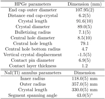
3.1 γγ-Coincidence Detector Dimensions . . . 37
3.2 Sum-Peak Attenuation Factors . . . 39
4.1 Beam-Induced Backgrounds . . . 47
4.2 18O Target Thickness . . . . 54
4.3 17O Target Thickness . . . . 56
5.1 Ex= 8084 keV Level Parameters . . . 61
5.2 18O(p,γ)19F Monte Carlo Reaction Rates . . . . 75
6.1 Table of Previous Measurements . . . 80
6.2 Accumulated17O(p,γ)18F Data . . . . 81
6.3 Singles and Coincidence Intensities . . . 83
6.4 ER= 518 keV Angular Correlations . . . 91
6.5 Partial Number of Reactions for ER= 518 keV . . . 92
6.6 Branching Ratios for ER = 518 keV . . . 92
6.7 17O(p,γ)18F Systematic Uncertainties . . . . 93
6.8 Resonance Strength for ER= 518 keV . . . 93
6.9 ER= 193 keV Angular Correlations . . . 95
6.10 Partial Number of Reactions for ER= 193 keV . . . 95
6.11 Branching Ratios for ER = 193 keV . . . 96
6.12 Resonance Strength for ER= 193 keV . . . 96
6.13 Broad Resonance Branching Ratios . . . 99
6.14 18F Spectroscopic Factors . . . 100
6.15 Estimated Total17O(p,γ)18F Branching Ratios . . . 101
6.16 Angular Correlation Calculations by Transition . . . 103
6.17 Beam-Induced Background Template Histograms . . . 105
6.18 Partial Number of17O(p,γ)18F Reactions . . . 108
6.19 Branching Ratios from Partial17O(p,γ)18F Reactions . . . 109
6.20 Total and Direct Capture S-Factors . . . 111
B.1 17O(p,γ)18F Sub-Threshold Resonance Parameters . . . 133
B.2 17O(p,γ)18F Resonance Parameters . . . 133
C.1 Clebsch-Gordan Coefficients for Wint R,D(θ) Terms . . . 140
C.2 Racah Coefficients for Broad Resonance and DC Interference Terms . . . 140
C.3 Z1 Coefficients for Broad Resonance and DC Interference Terms . . . 141
C.4 Angular Correlation for Broad Resonance and DC Interference Terms . . . 141
LIST OF FIGURES
1.1 Hertzsprung-Russell Diagram . . . 2
1.2 Presolar Grains . . . 3
1.3 Presolar Oxide Grain Groups . . . 4
1.4 Cool Bottom Processing . . . 5
1.5 M57: The Ring Nebula . . . 6
1.6 CNO Cycles . . . 7
1.7 Illustration of a Classical Nova . . . 8
1.8 Nova Delphini 2013 . . . 9
2.1 Direct Capture Drawing . . . 14
2.2 Gamow Peaks . . . 17
3.1 Low Energy Nuclear Astrophysics Motivation . . . 25
3.2 The Laboratory for Experimental Nuclear Astrophysics . . . 26
3.3 The JN Van de Graaff . . . 27
3.4 The ECR Ion Source . . . 28
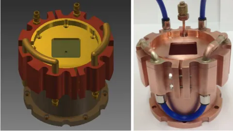
3.5 New ECR Ion Source Heat Sink . . . 31
3.6 New ECR Ion Source Dielectric Liner . . . 32
3.7 Degraded ECR Ion Source Acceleration Column . . . 33
3.8 Preliminary Pulsed Proton Beam Test . . . 34
3.9 Target Chamber . . . 36
3.10 Theγγ-Coincidence Spectrometer . . . 37
3.11 HPGe Peak Efficiencies . . . 41
3.12 γγ-Coincidence . . . 42
3.13 Theγγ-Coincidence Electronics . . . 46
4.1 Target Substrate . . . 48
4.2 Target Etching . . . 49
4.3 Target Resistive Heating . . . 50
4.4 New Anodization Chamber . . . 51
4.5 Assembled Anodization Chamber . . . 52
4.6 Anodized Oxygen Target . . . 53
4.8 17O Target JN Yield Curves . . . . 57
4.9 17O Target ECRIS Yield Curves . . . . 58
5.1 19F Level Diagram . . . . 60
5.2 Ex= 8084 keV Entrance and Exit Channel Angular Momenta . . . 61
5.3 ER= 95 keV Region of Interest . . . 63
5.4 Coincidence Correction Factor Assessment . . . 65
5.5 Resonance Strength PDF CL = 90% . . . 67
5.6 Direct Capture S-Factor at Ep = 105 keV . . . 69
5.7 Monte Carlo Reaction Rate PDFs . . . 71
5.8 (p,γ) Reaction Rate Comparison . . . 73
5.9 18O(p,γ)19F Reaction Rate Ratios . . . . 74
5.10 Reaction Rate Fractional Contributions . . . 75
5.11 (p,α) Reaction Rate Comparison . . . 77
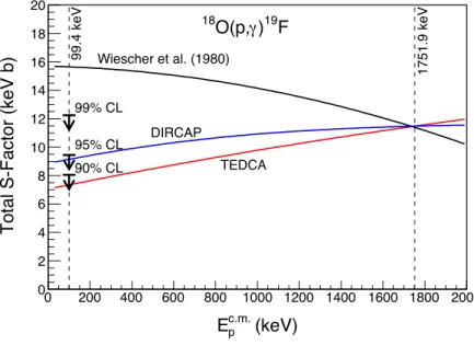
6.1 Literature Total S-Factors . . . 80
6.2 18F Level Diagram . . . . 82
6.3 Example Monte Carlo Resolution Functions . . . 86
6.4 rootSort Routine Flowchart . . . 87
6.5 TFractionFitterCode Flowchart . . . 90
6.6 Direct Capture and Broad Resonance Decay Schemes . . . 98
6.7 Breit-Wigner and DC Model Calculations . . . 99
6.8 Peak Intensity Ratio With and Without18F Correlations . . . 104
6.9 Example17O(p,γ)18F Fit at Ep= 250 keV . . . 107
6.10 New Total S-Factors . . . 111
6.11 New Direct Capture S-Factors . . . 113
6.12 Reaction Rate PDFs . . . 114
6.13 Interference Rate Comparison . . . 116
6.14 Analytical vs. Numerical Rate Comparison . . . 118
6.15 NACRE Rate Comparison . . . 120
6.16 2010 LENA Rate Comparison . . . 121
6.17 LUNA Rate Comparison . . . 122
6.18 Reaction Rate Contour Plot . . . 123
C.1 Computed Resonant and Direct Capture Cross Sections . . . 143
C.2 Longlandet al. (2006) Absorption Coefficients . . . 144
C.3 Resonant and Direct Capture Interference Sensitivity . . . 145
C.4 Resonant and DC (p→d) Interference Term . . . 146
C.5 tedcaCross Sections forℓf = 0 andℓf∗ = 2 . . . 149
C.6 Angular Correlation forℓf = 0 andℓf∗ = 2 . . . 150
C.7 tedcaCross Sections forℓi= 1 and ℓi∗ = 3 . . . 152
C.8 Angular Correlation forℓi = 1 andℓi∗ = 3 Interference . . . 153
D.1 Sum-Correcting with Geant4. . . 155
D.2 Monte Carlo Peak Efficiencies . . . 156
D.3 NaI(Tl) Annulus Gated Total Efficiency . . . 159
E.1 Ep = 175 keV Spectra . . . 162
E.2 Ep = 190 keV Spectra . . . 163
E.3 Ep = 250 keV Spectra . . . 164
E.4 Ep = 275 keV Spectra . . . 165
E.5 Ep = 300 keV Spectra . . . 166
E.6 Ep = 325 keV Spectra . . . 167
CHAPTER 1: INTRODUCTION
Section 1.1: Astrophysical Motivation
Visualizing stellar evolution is facilitated by acolor-magnitude diagramor Hertzsprung-Russell diagram. By plotting luminosity versus surface temperature (with decreasing temperature from right to left), the relationship between stellar mass, luminosity, surface temperature, age, and evolutionary stage can be un-derstood. Figure 1.1 [3] is a common example of a Hertzsprung-Russell diagram because it features a lot of structure that can be attributed to the different stages of stellar evolution. In this figure, the B−V color index is used instead of surface temperature, and absolute magnitude is used instead of luminosity. Impor-tant features are labeled in Fig. 1.1; when a star is burning hydrogen to helium in its core, it lies along the main sequence (MS). The Sun, for example, is a main sequence star, and at a core temperature of 15 MK, four protons fuse to helium and release a substantial amount of energy (along with two positrons and two neutrinos):
4H→4He + 2e++ 2ν+ 26.7 MeV. (1.1)
Based on the mass of a particular star, it may remain on the main sequence for millions to billions of years— more massive stars exhaust their supply of core hydrogen and evolve offthe main sequence before lower mass stars. The main sequence turn-offpoint (TO) is a luminosity versus temperature feature that corresponds to the age of a cluster. If it can be assumed that the stars in a cluster all formed at the same time, and the mass is proportional to the time spent on the main sequence (≈90% of the star’s lifespan), then the turn-off
and then hydrogen encase a carbon-oxygen core (an oxygen-neon core in more massive stars). During the asymptotic giant branch phase, recurrent periods of instability gradually drive offa star’s envelope creating a planetary nebula and exposing the electron-degenerate core, a stellar corpse called a white dwarf. Stars more massive than≈11 M⊙ (where M⊙ is the mass of the Sun) end their lives violently as supernovae producing a compact remnant—either a black hole or neutron star (depending on the mass of the progenitor).
Figure 1.1: From Ref. [3], the globular cluster M3 is the population of stars shown in this color-magnitude diagram. The x-axis is the B−V color index. Along the y-axis, the absolute magnitude is shown. The main sequence branch (MS), the main sequence turn-offpoint (TO), the red giant branch (RGB), the asymptotic giant branch (AGB), the horizontal branch (HB), and the post-asymptotic giant brand (P-AGB) are shown on this plot. These features correspond to different burning stages during stellar evolution. See Ref. [4] for more information on stellar evolution.
1.1.1: Cool Bottom Processing in Low-Mass AGB Stars
Matter in our solar system has a unique 18O/16O isotopic signature—(2.09+0.13
−0.12)×10−3 [5]. However,
a collection of presolar grain samples features peculiar oxygen isotopic ratios. Presolar grains are dust particles that condensed in the ejecta of evolved stars, supernovae, or, in some cases, classical novae [6] (see Fig. 1.2). These grains can be isolated from meteorites and then probed with secondary ion mass spectrometry (SIMS) or resonance ionization mass spectrometry (RIMS) [7]. Grains can provide insight into Galactic chemical evolution, stellar nucleosynthesis and evolution, and circumstellar and interstellar dust formation [8,6]. Certain alumina (Al2O3) grains are considered outliers with respect to the trove of presolar
grains gathered over the years from primitive meteorites and interplanetary dust particles. The18O study
Figure 1.2: From Ref. [9], (a) a scanning electron (SE) micrograph image of a 3µm presolar SiC grain, (b) a SE image of a 5µm presolar graphite grain, (c) a SE image of a 0.5µm presolar Al2O3 grain, and (d) a
high-resolution transmission electron microscope image of presolar nanodiamonds.
dust collapsed to form the nascent star. As the solar system cooled and the Sun ascended the main sequence, the presolar grains that survived were incorporated into primitive meteorites. The study of their abnormal isotopic ratios provides crucial constraints for astrophysical models. The18O(p,γ)19F portion of this thesis
focuses on oxide grains referred to asGroup 2 grains, approximately 15% of all presolar oxides [6] (see Fig. 1.3a). They exhibit a characteristic 18O/16O abundance ratio ≤1.5×10⁻³ [10], reflecting substantial 18O
depletion [7] with respect to the Solar value.
The depletion of 18O may occur due to cool bottom processing (CBP) [6] in low-mass red giant branch
(RGB) and asymptotic giant branch (AGB) stars [10]. This extra mixing process was proposed by Ref. [12] to account for isotopic anomalies, including 18O depletion, in presolar grains. During cool bottom
processing, material circulates between the convective envelope and the radiative zone that separates the envelope from the hydrogen burning shell (see Fig. 1.4). The base of the convective envelope remains cool, thus distinguishing this process from hot bottom burning (HBB) that occurs in 4−7 M⊙ asymptotic giant branch stars [12, 6]. Hot bottom burning peak temperatures range from 30 MK to about 100 MK and may be as high as 125 MK [14] (17O + p may impact hot bottom burning at these temperatures [15] and will be discussed later in Chapter 6). During cool bottom processing, as the circulated matter approaches the hydrogen shell, it reaches temperatures high enough to destroy 18O via hydrogen burning.
(a) (b)
Figure 1.3: (a) From Ref. [7], a plot of the different presolar oxide grains with 17O/16O on the y-axis and
18O/16O on the x-axis. The dashed lines represent the Solar values. The solid red circles, Group 2, represent
roughly 15% of all presolar oxides and exhibit extreme 18O depletion [6]. (b) From Ref. [11], a simplified
version where the T54 and C4-8 grains—thought to be produced by classical novae (see Sec. 1.1.2)—are emphasized. The abbreviations GCE, CBP, and HBB refer to Galactic chemical evolution, cool bottom processing, and hot bottom burning, respectively.
However, as pointed out by Refs. [28, 29], there is a finite amount of time during an evolutionary stage in which nucleosynthesis due to extra-mixing processes can occur and produce observed isotopic abundances. Mechanisms like magnetic buoyancy are fast and could satisfy this constraint [16,30,17], while diffusive and rotational processes are slow and less likely to drive cool bottom processing [31,32].
For a 1.0 M⊙≤M≤1.5−1.7 M⊙ red giant branch star, moderate18O depletion might occur due to cool
bottom processing, and this depletion is reflected in the Group 1 grains [33] in Fig. 1.3a [10]. According to Palmerini et al. (2011a) [10], cool bottom processing in RGB stars is a viable, but moderate, 18O
destruction mechanism if the maximum temperature of the circulated material approaches TP≈24 MK and
the hydrogen-burning shell is (at most) TH≈38 MK. Cool bottom processing in RGB stars can not account
for the Group 2 presolar grains in Fig. 1.3a [10], and there must be another stellar environment where cool bottom processing occurs [34]. It is hypothesized that low-mass asymptotic giant branch stars are this 18O
depletion site [6,10].
Principle,no more than two spin 1/2 particles can occupy a given quantum state simultaneously. Degenerate gas resists compression because all lower-lying states are occupied; pressure no longer depends on temperature [4]. During periods of helium-burning, referred to as thermal pulses, thermonuclear runaway (TNR) occurs and drives convection between the two burning sites. When the thermonuclear runaway subsides, the star compensates for this period of activity by expanding and cooling. The hydrogen burning shell is quenched during expansion, and the convective envelope dredges the products of nucleosynthesis to the surface of the star (third dredge-up). After this dredge-up event, the star contracts, and the hydrogen shell reignites. This interplay between the helium and hydrogen shells repeats episodically [35].
The18O depletion observed in Group 2 presolar oxide grains and AGB stellar atmospheres helped to
motivate the introduction of cool bottom processing into AGB stellar models. These models provided some insight into the class of asymptotic giant branch stars that might experience cool bottom processing and the temperature of the stellar plasma at the site of this extra mixing. According to Ref. [10],18O depletion
by cool bottom processing is possible in M ≤ 1.5 M⊙ asymptotic giant branch stars; temperatures of the circulated material between TP ≈ 38−48 MK, where the maximum H-burning shell temperature is TH ≈
Figure 1.4: Drawing, from Ref. [13], of the interior of an evolved star where cool bottom processing (CBP) occurs by some unknown extra mixing mechanism (not drawn to scale). The main regions are the C/O core, the He region, the H-burning region, the radiative zone, and the convective envelope. Material from the envelope slowly circulates deep into the radiative zone, and undergoes nuclear processing near the hydrogen shell. The processed material, now depleted in18O, circulates back into the envelope. The labels, M
BCE,
MP, and MH are the mass coordinates of the convective envelope boundary, the cool bottom processing
region, and the hydrogen shell, respectively. The other labels, TP, TH, and ˙M refer to the temperature
60 MK, are necessary to reproduce observed 18O/16O abundances [10]. Group 2 presolar grains nucleate
in the AGB stellar atmosphere depleted in 18O due to processes that occurred deep within the star—the
products of nucleosynthesis were dredged up to the surface of the star. Then, powerful stellar winds inject these grains into the interstellar medium.
Figure 1.5: M57: the Ring Nebula [37], a planetary nebula with a central white dwarf that was produced after an asymptotic giant branch star shed its convective envelope [38].
The depletion of18O in a stellar plasma at low temperatures is driven by 18O(p,α)15N and, to a lesser
extent,18O(p,γ)19F. These two18O destruction mechanisms are a part of the CNO cycle (see Fig. 1.6b). The
(p,α) reaction was recently studied indirectly by Ref. [39]. Within the cool bottom processing temperature regime, the 18O(p,γ)19F reaction rate may be influenced by an unobserved, low-energy resonance at E
R
= 95 ± 3 keV [40, 41] (see Fig. 5.1). Note that all bombarding and resonance energies reported in this thesis are in the laboratory reference frame unless noted otherwise. In the present work, a direct, low-energy measurement of the 18O(p,γ)19F reaction is reported. The goal of this measurement was to improve our
knowledge of levels in the19F compound nucleus relevant to nuclear astrophysics.
1.1.2: Explosive Hydrogen Burning During Classical Novae
(a) (b)
Figure 1.6: (a) The Hot CNO cycle is activated during explosive hydrogen burning in classical novae. The main reaction channels are (p,γ), (p,α), and (β+ν). The Hot CNO cycle is shown with red arrows in this
figure, and the17O(p,γ)18F reaction is highlighted with blue squares. (b) Extreme18O depletion is possible
if the CNO cycle is activated during cool bottom processing in low-mass asymptotic giant branch stars. The main destruction channels are the (p,γ) and (p,α) reactions. The CNO cycle of interest is shown with red arrows in this figure, and the 18O(p,γ)19F reaction is highlighted with blue squares. The competing 18O(p,α)15N path is also shown with a green arrow, and15N is highlighted in blue.
layers of matter exposing a compact stellarcorpse. These remnants, depending on the mass of the original star, are primarily carbon and oxygen. In a binary star system, this stellar corpse, referred to as a white dwarf star, can be reanimated by its companion. As the companion evolves, a parasitic white dwarf will begin to leach hydrogen-rich matter from the host main sequence star by Roche lobe overflow through the inner Lagrangian point of the binary system. An accretion disk can form around the white dwarf (if the magnetic field is weak), and layers of accreted hydrogen build up on the surface of the compact remnant. As more matter is accreted, compression will drive the underbelly of this hydrogen layer into a state of degeneracy. As stellar plasma temperatures rise, there is no longer a mechanism in place to cool the accreted material, and a thermonuclear runaway occurs [44,42]. Thermonuclear reactions will proceed rapidly over a period of about 100 seconds, and during the outburst, the luminosity can increase by as much as a factor of 10,000 [45]. With luminosities between 1045−1046ergs [46], classical novae are only surpassed in luminosity
by supernovae, hypernovae, andγ-ray bursts [42]. To put this in perspective, the AN602 hydrogen bomb (also known asTsar Bomba), the most powerful nuclear weapon ever detonated, had an estimated yield of
≈2.38×1024ergs [47]. White dwarfs have diameters that are the same order of magnitude as the diameter of
Figure 1.7: An artist’s interpretation of a classical nova ( c⃝ David A. Hardy/www.astroart.org [43]). It depicts a white dwarf accreting matter from a bloated main sequence star. Roche lobe overflow has formed an accretion disk around the white dwarf.
bombs would have to detonate on every square centimeter of Venus to match the output of a classical nova [48].
Unlike supernovae, classical novae are recurrent events—the star system is not disrupted and thermonu-clear runaway can reoccur with a period of 104−105 years [45]. The most common classical novae involve
a carbon-oxygen (CO) white dwarf that originated from a main sequence star≤9−10 M⊙. Heavier white dwarf stars from more evolved progenitors are classified as oxygen-neon (ONe) white dwarfs based on the nuclear ash accumulated during the progenitor’s stellar evolution. Classical novae should not be confused withdwarf novae ornovae-like variables; these recurrent variables are not thermonuclear burning sites. X-ray novae, on the other hand, are analogous to classical novae, but involve an accreting black hole or neutron star in a binary system instead of a white dwarf [42]. Classical novae occur in the Milky Way Galaxy at a rate of 35±11 novae/year [49]. Figure 1.8 is an image taken of the recent nova, Nova Delphini 2013, with a PlaneWave 17” unit.
Figure 1.8: An image taken with a PlaneWave 17” unit, after the average of 10, 10-seconds unfiltered exposures of Nova Delphini 2013. The classical nova is the bright object dominating the center of the frame [50].
(p,γ), (p,α), and (β+ν) paths [42]. Because the timescale—100 seconds—is so short, the CNO cycle never
reaches equilibrium [44], and convection transportsβ+ unstable nuclei to the surface of the envelope. These
nuclei contribute the energy necessary to increase temperature and entropy to the point at which envelope degeneracy is lifted (the Fermi temperature), halt the thermonuclear runaway, and drive expansion and the ejection of the products of nucleosynthesis. They are also the slowest paths during the Hot CNO cycle and are essentially the nova nucleosynthesis bottleneck [42]. Classical nova peak temperatures range between 100−400 MK [52,53,54], and this defines the classical nova Gamow window—the temperature regime that needs to be probed experimentally.
Based on stellar models, reaction networks, and astronomical observations, novae are thought to be significant sources of Galactic 13C, 15N, and 17O [55, 52, 54], and ≈1/3000 the Galaxy’s disk dust and
gas [42]. Classical novae also produce 7Li, 19F, and 26Al, but CNO elements are the dominant products
[53, 54]. One of the major elements created during the explosion is18F. It is not a stable fluorine isotope
and decays by emitting a positron. When the positron encounters an electron, they annihilate producing radiation with a specific energy (511 keV) [56,57]. Because the half-life of18F is≈110 minutes, the 511 keV γ-ray is produced after the classical nova envelope has become transparent to γ-rays. Other β+ unstable
nuclei, like 13N, decay while the envelope is opaque to γ-rays and their associated 511 keV γ-rays drive
envelope expansion. The 511 keV signature from 18F would be important to observe with an astronomical
instrument likeintegral, because detection could constrain classical nova models [58]. However, detectors like integral would need to get lucky and be pointed at the right portion of the sky to detect these 18F
Stellar models could also be constrained by studying nova presolar grains. Presolar grains could form in the cool, low-density envelope ejected by classical novae [42]. Infrared [59,60] and ultraviolet [61] observations of nova light curves indicate dust formation, and suggest that CO-type novae are prolific dust creators [62,63] while ONe-novae are not. This may be due to high-velocity ejecta from these novae and lower envelope densities. These grains should have anomalous carbon and nitrogen ratios [64], and oxygen isotopic ratios in these grains could constrain the type of nova that produced them, the mass of the white dwarf, and mixing processes between accreted and core matter [42]. Mixing occurs between core and accreted matter by some unknown mechanism [65]; candidate mixing methods include shear mixing [66,67, 68,69], elemental diffusion [70,71], and the Kelvin-Helmholtz instability [72]. Grains that can be attributed to classical novae are rare (see Fig. 1.3b). The criteria are: (1) observation of17O enrichment with17O/16O>0.004 and (2) mild18O depletion [7]. Alumina grain T54 [33] is one grain considered consistent with nova nucleosynthesis
calculations [73]—17O/16O = 1.41×10⁻² [11]. Grain C4-8 is another nova grain candidate with 17O/16O
= 4.4×10⁻² (an order of magnitude higher than the concentration allowed by low-mass asymptotic giant
branch models) [11]. Both grains are likely from CO-novae because18O/16O abundance ratios are too high
to attribute the grains to ONe-novae [11]. Nova grains are large compared to grains from the interstellar medium (ISM); nova grains are typically on the order of≈0.5µm [74]. The only known nova remnant that shows any indication of dust and molecules is GK Persei, but it is not thought that these grains are related to the 1901 nova event [74].
It is clear that thermonuclear reactions that create and destroy18F are extremely important and need
to be studied experimentally. The most important18F production mechanism is the capture of a proton by 17O (the rarest stable oxygen isotope). This reaction also affects the destruction of17O, and classical novae
are thought to be the dominant source of17O in our Galaxy. However, there is evidence in the literature
that hot bottom burning in asymptotic giant branch stars may also contribute to the synthesis of17O [15]
where T = 30−100 MK [75].
The importance of 17O proton capture—17O(p,γ)18F—is well established, and numerous studies have
been performed to analyze this reaction experimentally [51,76]. However, the temperature regime relevant to explosive hydrogen burning during a classical nova (100−400 MK) corresponds to very low proton bom-barding energies (Ecm
during classical novae, the experimental tools at the LENA facility allow17O proton capture reaction rates
to be constrained. In particular, direct capture is studied because reaction rate calculations indicate that direct capture dominates the rate at classical nova temperatures [75, 78]. This is a rare scenario because generally, narrow resonances at astrophysically relevant temperatures dominate the rate [78].
Section 1.2: Focus
In the following chapters, both (p,γ) experiments are described in detail. Chapter 2 outlines a majority of the underlying nuclear physics that affects how both experiments were designed and executed, and how data were analyzed. Chapter 3 describes the laboratory facility, the accelerators, and the detector system. Within chapter 3, relevant upgrades and modifications are discussed along with calibrations of the key equipment used in these studies. Target fabrication and characterization for both studies are discussed in Chapter 4. Then, Chapter 5 focuses specifically on the18O(p,γ)19F experiment while Chapter 6 is dedicated
to measurement, analysis, and results of the 17O(p,γ)18F direct capture study. The results presented in
CHAPTER 2: NUCLEAR ASTROPHYSICS THEORY
The fundamental nuclear astrophysics concepts and equations outlined in this chapter are adapted from the text Nuclear Physics of Stars by C. Iliadis [4] and references therein. The equations presented in this chapter are used throughout the remainder of this dissertation and are key components to the analysis developed in this work and in preceding studies done at LENA. Note that stellar plasma energies, bombarding energies, and resonance energies discussed in this chapter are in the center-of-mass frame. In subsequent chapters, it should be assumed that all energies are in the laboratory frame.
Section 2.1: Thermonuclear Reaction Rates
Thermonuclear reaction rates are a quantitative measure of nuclear reaction probabilities in a stellar plasma. Thermonuclear reaction rate theory is discussed here as are the applications of this theory to the study of rare oxygen isotope proton captures.
The physical quantity at the heart of these studies, the main piece of nuclear physics information that these experiments are dedicated to measuring in the laboratory, is the nuclear cross section. This quantity, σ, is the probability that a nuclear interaction occurs between target nuclei and incident particles, and it can be defined as:
σ= interactions per unit time
incident particles per unit time×target nuclei per unit area. (2.1)
The cross section is expressed in units of barns (b) where
1 b = 10−24cm2, (2.2)
and as the units imply, this probability is essentially an area—the interaction area of target nuclei and incident particles. References to the cross section in this thesis will be limited to radiative proton capture. This means that the incident particles in the reactions discussed in this dissertation are protons, and when target nuclei capture these protons, electromagnetic radiation—aγ-ray—is emitted.
φ(v). The reaction rate per particle pair is thus a convolution between the cross section and the velocity distribution where:
<σv>=
! ∞
0
φ(v)vσ(v)dv. (2.3)
The velocity distribution is assumed to be a Maxwell-Boltzmann distribution,
φ(v) =
" µ
2πkT
#3/2
e−µv2/(2kT)
4πv2, (2.4)
if the reaction rate describes the interaction of non-degenerate, non-relativistic particles. Where
E = µv
2
2 (2.5)
and
µ= MpMt
Mp+ Mt (2.6)
is the reduced mass of the target nucleus and incident particle (Mt and Mp, respectively), Eq. 2.3 can be rewritten as:
<σv>=
"
8 πµ
#1/2
1 (kT)3/2
! ∞
0
σ(E)Ee−E/kTdE. (2.7)
In this equation, the Boltzmann constant, k, is equal to 8.6173×10⁻⁸keV/K. The thermonuclear reaction
rate at a specific stellar plasma temperature can be calculated numerically with the following equation:
NA<σv>=
3.7318×10¹⁰√µ
T93/2
! ∞
0
σ(E)Ee−11.605E/T9dE (cm3mol−1s−1). (2.8)
In this equation, E is the center-of-mass energy in units of MeV, T9 is the temperature in GK, and the
cross section is in barns. The nuclear masses are calculated from the atomic masses listed in Ref. [41] by subtracting the mass of electrons associated with the projectile and target atoms; all masses are in atomic mass units.
2.1.1: Non-Resonant Reaction Rates
core instead of a collection of individual nucleons; the reaction is not as sensitive to the nuclear interior and strong nuclear force as it is to the nuclear exterior and the electromagnetic force. The direct capture cross section varies smoothly as a function of energy because of this reaction mechanism’s dependence on the electromagnetic force. The energies of direct capture primary transitions can be calculated with the equation:
Eγ = Qpγ+ Ep−Ex (2.9)
where Eγ is the energy of a single direct capture primary, Qpγ is the proton separation energy of the target
nucleus for a (p,γ) reaction, Ep is the center-of-mass energy of the proton, and Exis the bound state energy.
Figure 2.1: FromCauldrons in the Cosmos by Rolfs and Rodney [83], an incident particle capturing from an initial scattering state directly into a final bound state of nucleus “A.”
The E1 transition is the dominant contribution to the direct capture cross section, and it can be described with the following equation:
σcalc(E1) =0.0716µ3/2
"Z
p Mp −
Zt Mt
#2 E3
γ
E3p/2
× (2.10)
(2Jf+ 1)(2ℓi+ 1) (2jp+ 1)(2jt+ 1)(2ℓf+ 1)
(ℓi010|ℓf0)2R2ℓi1ℓf. (2.11)
is the radial integral where
Rℓi1ℓf =
! ∞
0
uc(r)OE1(r)ub(r)r2dr (2.12)
and in this equation, OE1(r) is the radial part of the E1 electric dipole operator, and uc and ub are the continuum and bound state wave functions, respectively [84, 85].
The energy dependence of the direct capture cross section can be attributed to the radial integral,Rℓi1ℓf,
because the radial wave functions of the initial scattering and final bound states are sensitive to the energy. This means the scattering and bound state potentials selected to describe the nuclear potential are very important. IfJf,jp, andjtare known, the initial and final orbital angular momenta can be calculated. These values were calculated for both the18O(p,γ)19F and17O(p,γ)18F reactions, but as an example, 17O(p,γ)18F
coupling calculations are discussed here:
17O +p+ℓi
→ 18F + E1; (2.13)
17O +p+ℓf
→ 18F. (2.14)
Consider 17O proton capture and the formation of a 3+ state in 18F. The proton and 17O have angular
momenta of 12+ and 52+ , respectively, and they can couple to a total momentum of 2+ or 3+. The E1 multipolarity and18F have angular momenta of 1− and 3+, respectively, and they can couple to 2−, 3−, or
4−. As a result,ℓimust be odd because the final parity is proportional to (-1)ℓ. The possible initial angular
momenta are 1, 3, 5, or 7, but usually, all but the first twoℓvalues are excluded from a coupling calculation. Equation 2.14 can be solved for ℓf with a similar procedure. The formation of the final angular momen-tum, 3+, requires thatℓf be even, and this allowsℓf = 0 or 2; the final possible combinations areℓi = 1, 3
andℓf = 0, 2. The coupling calculations provide the quantities necessary to calculate the initial scattering and final bound state wave functions. The accepted17O(p,γ)18F direct capture coupling calculation solutions
are tabulated in Tab. 2.1.
Table 2.1: The17O +pchannel spin, total angular momentum of direct capture states, and the corresponding
initial scattering state and final bound state orbital angular momenta.
s Jπ ℓi ℓf
2 0+ (1,3) 2
3 1+ (1,3) 2
2 2+ (1,3) (0,2)
3 3+ (1,3) (0,2)
2 4+ (1,3) 2
For direct capture, the scattering state potential is set to zero [85], and the Woods-Saxon potential:
VW S(r) = −
V0
1 +er−Ra
(2.15)
whereR=r0A1t/3,r0 = 1.25 fm, anda= 0.65 fm [85], is chosen for the bound state potential.
The assumption made in the direct capture formalism—that the target nucleus can be approximated as a single particle—is not entirely correct. Only a fraction of the total wave function exists as a single particle state. Spectroscopic factors are an empirical estimate of what fraction of the final state wave function can be described by a single particle bound in a potential well. The experimental cross section is related to the theoretical cross section by
σexp=
$
ℓi,ℓf
C2S(ℓf)σtheo(ℓi,ℓf). (2.16)
The summation in this equation is over all possible initial and final state orbital angular momenta,ℓi and ℓf, and C2S(ℓf) is the spectroscopic factor—the probability of arrangement into a residual nucleus and a
single particle [4].
The smoothly varying direct capture cross section drops dramatically at low energies due to Coulomb suppression, and this exponential decline makes it difficult to visualize and understand the nuclear physics at the energies most relevant to nuclear astrophysics. Because of this, non-resonant cross sections are often rewritten in terms of the astrophysical S-factor, S(E). This representation of the cross section is easier to grasp conceptually and plot because it excludes the steep energy dependence (1/E) and the Coulomb barrier transmission probability. It isolates the nuclear contributions to the cross section from the electromagnetic contributions. This decomposition of the cross section can be expressed as:
σ(E) = S(E) E e−
2πη (2.17)
where e−2πη is the Gamow factor andη is the Sommerfeld parameter. The 2πη term in the Gamow factor
can be written numerically as:
2πη= 0.98951013×
" ZpZt
% µ
E
#
(2.18)
where E is the center-of-mass energy in units of MeV.
The thermonuclear reaction rate can be rewritten in terms of the astrophysical S-factor by substituting Eq. 2.17 into Eq. 2.7 and multiplying by Avogadro’s number, NA:
NA<σv>=
"
8 πµ
#1/2
NA
(kT)3/2
! ∞
0
Within this integral is a very important quantity and concept in nuclear astrophysics, the Gamow peak. The product of the Gamow factor and the Maxwell-Boltzmann distribution, e−2πηe−E/kT, describes an energy range and stellar plasma temperature regime that contains the non-resonant reactions that dominate the reaction rate. If the derivative of this product is set to zero, the maximum value, E0 can be calculated:
E0= 0.122×(Zp2Zt2µT92)1/3 (MeV). (2.20)
Assuming the Gamow peak is normally distributed, the 1/ewidth of the peak can be written as:
∆E = 0.2368×(Zp2Zt2µT95)1/6(MeV). (2.21)
In Fig. 2.2, the Gamow peak is solved and plotted at T = 50 MK (cool bottom processing), T = 125 MK (hot bottom burning), and T = 300 MK (classical novae).
(keV)
p c.m.
E
0 100 200 300 400 500 600 700 800 900 1000
Probability (arb. units)
-25 10
-23 10
-21 10
-19 10
-17 10
-15 10
-13 10
-11 10
-9 10
-7 10
-5 10
-3 10
-1 10
10
GF
CBP
HBB
Novae
Figure 2.2: The products of the Gamow factor (solid black line) and the Maxwell-Boltzmann distributions (dashed lines) are plotted in this figure. The classical nova (blue), the hot bottom burning (red), and cool bottom processing (purple) Gamow peaks are shown as dotted lines. These peaks correspond to 300 MK, 125 MK, and 50 MK, respectively.
The astrophysical S-factor can be expanded in a Taylor series at E = 0 [86] because, with respect to energy, it is a slowly varying function:
S(E)≈S(0) + ˙S(0)E +1 2S(0)E¨
where ˙S(0) and ¨S(0) are the first and second derivatives of S(E) at E = 0 keV, respectively. An analytical expression for the non-resonant reaction rate can be written as:
NA<σv>=
"4
3
#3/2 !N
A
πµZpZte2Sef fτ
2e−τ (2.23)
where
τ =3E0
kT = 4.2487×
"Z2
pZt2µ
T9
#1/3
(2.24)
and the effective S-factor [86] is
Sef f(E0) = S(0)
&
1 + 5 12τ +
˙S(0) S(0)
"
E0+35
36kT
#
+1 2 ¨ S(0) S(0)
"
E20+
89 36E0kT
#'
. (2.25)
If Eq. 2.22 diverges at high energies and fails to reproduce experimental data, the non-resonant reaction rate is multiplied by a cutofffunction,
fcutoff≈e−(T9/T9,cutoff) 2
, (2.26)
to dampen its affect at these energies. In this equation,
T9,cutoff= 19.92×
(
E3cuto/2ff
) Z2
pZt2µ
*
(2.27)
where Ecutoff is in units of MeV.
2.1.2: Resonant Reaction Rates
Resonant captures, as opposed to direct captures, have energy-dependent cross sections—they do not vary smoothly. Variations in the cross section can span orders of magnitude over very narrow energy ranges. The total cross section thus resembles a smoothly varying background interspersed with spikes—resonances superimposed upon the direct capture cross section. Unlike direct capture, the nuclear interior plays a major role during resonant capture. At energies near the quasi-bound state potential energies, the matching of solutions to the interior and exterior wave function at the nuclear radius is favorable, and this produces a large wave function amplitude in the nuclear interior. This matching condition is satisfied when the sum of the resonance energy, ER, (in the center-of-mass frame) and proton separation energy equals the excited
state energy,
Narrow Resonances
Narrow resonances have constant partial widths (Γa,Γb) over the total width (Γ)—the sum of all partial widths—of the resonance. The total width of a narrow resonance is typicallyΓ<1−3 keV. The Breit-Wigner equation can be used to express a resonant cross section where
σBW(E) = λ
2
4πω
ΓaΓb
(E−ER)2+ (Γ/2)2 (2.29)
and
ω= 2J+ 1 (2Jp+ 1)(2Jt+ 1)
. (2.30)
In these equations, Jp is the projectile spin,Jt is the target spin,J is the spin of the resonance state, ER
is the resonance energy in the center-of-mass frame, Γa is the entrance channel partial width,Γb is the exit channel partial width,Γis the total resonance width, and λis the de Broglie wavelength, defined as
λ= √2π!
2µE. (2.31)
The single resonance reaction rate then becomes
NA<σv>=NA
√
2π!2 (µkT)3/2ω
! ∞
0
ΓaΓb
(ER−E)2+Γ2/4e
−E/kTdE (2.32)
when the Breit-Wigner cross section and de Broglie wavelength are substituted into Eq. 2.7 and then multiplied by Avogadro’s number. If the Maxwell-Boltzmann distribution and partial widths are assumed to be constant, the narrow resonance reaction rate can be simplified further to
NA<σv>=NA
√
2π!2 (µkT)3/2e−
E/kTω2ΓaΓb
Γ
! ∞
0
Γ/2
(ER−E)2+Γ2/4
dE. (2.33)
This integral simplifies toπbecause
! ∞
−∞
a
(ER−E)2+a2dE =π, (2.34)
and an analytical expression for the narrow resonance reaction rate can be written as
NA<σv>=NA
"√2π
µkT
#3/2
where the resonance strength is defined as
ωγ=ωΓaΓb
Γ . (2.36)
Broad Resonances
The cross section of a broad resonance varies over wider energy ranges than are typical for narrow resonances. A good rule of thumb for resonances within the Gamow window is: if the total width, Γ, is a significant fraction of the Gamow peak width, the resonance is a broad resonance. Because of the inherent energy dependence of the broad resonance cross section, the partial widths, de Broglie wavelength, and the Maxwell-Boltzmann distribution can not be assumed to be constant, and the broad resonance reaction rate becomes
NA<σv>=NA
√
2π!2 (µkT)3/2ω
! ∞
0
Γa(E)Γb(E +Sp−Ef) (ER−E)2+Γ(E)2/4
e−E/kTdE. (2.37)
In this equationΓb corresponds to the partial width of a single exit channel transition andSp is the proton separation energy. Multiple transitions sum incoherently with the cross section, and broad resonance tails are also included in the rate calculation. The energy dependence of the entrance channel partial width can be approximated by the penetration factor,Pa(E)—the transmission probability through the Coulomb and centripetal barriers:
Γa(E) =Γa(ER)
Pa(E)
Pa(ER)
. (2.38)
The exit channel partial width becomes:
Γb(E) =Γb(ER+Sp−Ef)
Pb(E +Sp−Ef)
Pb(ER+Sp−Ef)
. (2.39)
Assuming the exit channel is aγ-ray, as is the case in these experiments,
Γb(E) =Γγ(ER+ Qpγ−Ef)
&
E + Qpγ−Ef
ER+ Qpγ−Ef
'2L+1
(2.40)
becauseΓγ ≈E2γL+1 (whereLis the multipolarity of the emittedγ-ray). HereSp = Qpγ. By making these
substitutions, the Breit-Wigner cross section for a (p,γ) reaction becomes:
σBW(E) =π!
2ω
2µE
Γa(ER)PPaa(E(E)R)Γγ(ER+ Qpγ−Ef)
&
E+Qpγ−Ef ER+Qpγ−Ef
'2L+1
(ER−E)2+Γ(E)2/4 . (2.41)
For sub-threshold resonances (Ecm
factor, C2S, and the single particle reduced width, θ2
sp [87]—the probability of a single nucleon appearing on the nuclear boundary. Spectroscopic factors are generally well documented in the literature by studies of stripping reactions—like (d,n) or (3He,d). The particle partial width becomes
Γp(E) = 2!
2
µR2P(E)C
2Sθ2
sp (2.42)
where the majority of the energy dependence comes from the penetration factor.
Interfering Resonances
If two or more resonances have the same spin and parity, the amplitudes of these resonances can interfere either constructively or destructively. For two interfering resonances, the cross sections sum coherently where the total cross section is defined as
σ(E) =σ1(E) +σ2(E)±2
+
σ1(E)σ2(E)cos(δ1−δ2) (2.43)
and the phase shift of each resonance can be generalized as
δi=arctan
& Γ
i 2(E−ER,i)
'
. (2.44)
The interference cross section can be substituted into Eq. 2.7, and this single reaction rate replaces the incoherent sum of the interfering resonances in the total reaction rate calculation. If the total widths of the interfering resonances are narrow (Γi <1 eV), an argument can be made for ignoring the interference.
Finally, the total reaction rate is the incoherent sum of the non-resonant (NR), narrow resonance (RN), broad resonance (RB), and continuum (C) reaction rates:
NA<σv>total=NA<σv>N R+
$
i
NA<σv>RNi +
$
j
NA<σv>RBj +NA<σv>C. (2.45)
Section 2.2: Monte Carlo Reaction Rates
2.2.1, resonance energies are assumed to be normally distributed (Gaussian), resonance strengths, S-factors, and partial widths are lognormal distributions, and upper limits are treated as Porter-Thomas distributions. The final reaction rate probability density function is a lognormal distribution where the 0.16, 0.50, and 0.84 quantiles of the cumulative PDF are adopted as the low, median, and high reaction rates, respectively. The low and high rate are bounds that correspond to 68% coverage or 1σ, and can be referred to as the
uncertaintyin the rate. However, this uncertainty is used to describe the reaction rate probability density function—a continuum that the actual rate lies upon—and is not meant to be considered ahard-cut-off—the probability that the rate lies above the high rate or below the low rate is non-negligible.
2.2.1: Probability Density Functions
The quantities that factor into these Monte Carlo reaction rate calculations are associated with probability density functions. However, there are several key caveats that must be considered. Based on the nature and characteristics of an input parameter, an appropriate probability density function must be selected.
Resonance energies are assumed to be normally distributed (Gaussian), and in general, a Gaussian distribution is used when the uncertainty associated with a parameter can be considered the sum of many small contributions. For a continuous random variablex, the Gaussian function is defined as
f(x) = 1
σ√2πe −1
2
,x−µ
σ
-2
(2.46)
where µis the mean and, in this case, expectation value, andσ is the standard deviation (the square-root of the variance). The expectation value and variance can be generalized as
E[x] =
! ∞
−∞
xf(x)dx (2.47)
and
V[x] =
! ∞
−∞
(x−E[x])2f(x)dx, (2.48)
respectively.
distribution (0≤ x <∞). The lognormal distribution is defined as
f(x) = 1
σ√2π 1
xe
−12
,ln(x)−µ
σ
-2
(2.49)
where
µ= ln(E[x])−12ln
"
1 + V[x]
E[x]2
#
(2.50)
and
σ=
.
ln
"
1 + V[x]
E[x]2
#
. (2.51)
The geometric mean of a lognormal distribution is also the median where
µg =eµ. (2.52)
The geometric standard deviation is a lognormal distribution’s factor uncertainty and is defined as
σg=eσ. (2.53)
Upper and lower bounds, providing 68% coverage, are given byeµ±σ.
CHAPTER 3: ACCELERATORS AND DETECTORS
The Laboratory for Experimental Nuclear Astrophysics (LENA) is located on the campus of Duke Univer-sity, Durham, NC and operates under the aegis of Triangle Universities Nuclear Laboratory (TUNL). LENA is a “sea-level” accelerator facility dedicated to the measurement of nuclear cross sections within the energy regime relevant to nuclear astrophysics. Nucleosynthesis occurs within a stellar environment at energies that most accelerator facilities are incapable of probing. The main problem is that at low bombarding energies, the cross section drops dramatically because of decreasing transmission probability through the Coulomb barrier. As a result, experimental count rates drop below detectable thresholds unless great lengths are taken to design an experiment that can reduce environmental backgrounds and boost the reaction yield. Figure 3.1, courtesy of Ref. [4] (with data from Ref. [91]), demonstrates this conundrum quite well. In the figure, the
16O(p,γ)17F cross section decreases by approximately four orders of magnitude over a narrow energy window
(≈500 keV). The impact this has on detecting the characteristicfingerprintof a reaction in the laboratory is staggering; however, LENA is equipped to tackle these complications with its advanced accelerators and detectors. Note that Fig. 3.1 also shows the astrophysical S-factor. As discussed in Sec. 2.1.1, the S-factor is related to the cross section; to calculate the S-factor, the energy dependence and transmission probability are removed from the cross section.
Figure 3.2 shows the layout of the LENA facility including the accelerators, beamline, quadrupole magnets (blue), analyzing magnet (yellow), and steerers (black). The quadrupoles and steerers are optical elements that allow the beam to be focused and repositioned, respectively. Beam produced by each accelerator is transmitted through two sets of quadrupoles and steerers with an analyzing magnet between them. The analyzing magnet—at least during JN operation—is a key component in a National Instruments LabVIEW controlled feedback system that uses beam current measurements on horizontal slits downstream from the magnet to adjust the JN terminal voltage. The following equation determines the calibrated magnetic field:
B = k
q(2mc
2E + E2)1/2 (3.1)
Stellar ROI
Figure 3.1: An illustration of the major challenge and motivation behind experimental nuclear astrophysics from Ref. [4] (with data from Ref. [91]). The 16O(p,γ)17F cross section and S-factor are shown from
![Figure 1.3: (a) From Ref. [7], a plot of the different presolar oxide grains with 17 O/ 16 O on the y-axis and](https://thumb-us.123doks.com/thumbv2/123dok_us/8291787.2195786/23.918.122.807.93.397/figure-ref-plot-different-presolar-oxide-grains-axis.webp)
![Figure 3.8: From Ref. [92], a comparison between (a) the pulsed ECR ion source proton beam (measured at the first beamstop) and (b) the signal applied to the ion source high voltage supplies.](https://thumb-us.123doks.com/thumbv2/123dok_us/8291787.2195786/53.918.265.652.735.1010/figure-comparison-proton-measured-beamstop-applied-voltage-supplies.webp)