Compact appearance in object populations using quantile function based distribution families

(1)

Compact Appearance in Object Populations Using Quantile

Function Based Distribution Families

Robert Elijah Broadhurst

A dissertation submitted to the faculty of the University of North Carolina at Chapel Hill in partial fulfillment of the requirements for the degree of Doctor of Philosophy in the Department of Computer Science.

Chapel Hill 2008

Approved by:

(2)

c 2008

(3)

ABSTRACT

ROBERT ELIJAH BROADHURST: Compact Appearance in Object Populations Using Quantile Function Based Distribution Families

(Under the direction of Stephen M. Pizer)

Statistical measurements of the variability of probability distributions are important in many image analysis applications. For instance, let the appearance of a material in a picture be represented by the distribution of its pixel values. It is necessary to model the variability of these distributions to understand how the appearance of the material is affected by viewpoint, lighting, or scale changes. In medical imaging, an organ’s appearance varies not only due to the parameters of the imaging device but also due to changes in the organ, either within a patient day to day or between patients. Classical statistical techniques can be used to study distribution variability, given a distribution representation for which variation forms linear subspaces. For many distributions relevant to image analysis, standard representations are either too constrained or have nonlinear variation, in which case classical linear multivariate statistics are not applicable. This dissertation presents general, non-parametric representations of a variety of distribution types, based on the quantile function, for which a useful class of variability forms linear subspaces. A key consequence is that principal component analysis can be used to efficiently parameterize their variability, i.e., construct a distribution family.

(4)

(5)

ACKNOWLEDGMENTS

First and foremost, this document could not have been completed without the immense amount of time happily given by my advisor, Stephen M. Pizer. The quality of this document reflects his motivating influence. My other committee members, Edward Chaney, Leonard McMillan, Carlo Tomasi, and Andrew Nobel, were also very helpful in putting the final touches on this document. The below quote compactly expresses by gratitude to them.

“I have made this letter longer than usual, only because I have not had the time to make it shorter.” ∼Blaise Pascal

The research contained in this dissertation reflects how Steve and Ed picked me up when I first arrived in Chapel Hill in 2002. They stuck with me to the end, and I am thankful. This work could also not have been completed without the collaborations with all of the past and present members of the Medical Image Display and Analysis Group. Funding for this work was provided by National Institutes of Health grant P01 EB02779.

(6)

LIST OF TABLES

3.1 QF-QDA Classification results using the MR8 filter bank. . . 76

3.2 MR8 based QF-QDA accuracy constrained to equal projection error versus equal component number. . . 83

3.3 Classification results using Strong-MRF. . . 87

3.4 Classification results using PCA-MRF. . . 92

4.1 The benefit of statistically trained appearance functions. . . 132

4.2 Global versus local segmentation results for the bladder. . . 134

4.3 Global versus local segmentation results for the prostate. . . 134

4.4 Global versus local segmentation results for the bladder and prostate. . . 134

(11)

LIST OF FIGURES

2.1 Non-parametric representations of several common distributions. . . 10

2.2 Quantile functions as adaptive bin histograms. . . 15

2.3 The sensitivity of non-parametric representations to bin count. . . 16

2.4 Linear interpolation of non-parametric representations. . . 19

2.5 PDF and QF representations of location and mixture interpo-lated delta distributions. . . 22

2.6 Manifolds and distances of Gaussian distributions . . . 26

2.7 Manifolds and distances of Gaussian mixture distributions . . . 27

2.8 Manifolds and distances of gamma distributions . . . 28

2.9 Manifolds and distances of beta distributions . . . 29

2.10 Manifolds and distances of Weibull distributions . . . 30

2.11 Construction of orthogonal basis vectors in QF space. . . 33

2.12 Construction of the Weibull distribution. . . 34

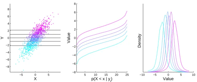
2.13 The QF based representation of conditional distributions. . . 46

3.1 The 61 materials in the CUReT database. . . 63

3.2 The “Zoomed Plaster B” material in CUReT. . . 64

3.3 The MR8 filter bank. . . 71

3.4 An example of PCA on QFs from filters in CUReT. . . 75

3.5 QF-QDA compared to previous work for smaller training sets . . . 77

3.6 Varying training set and QF size for QF-QDA, QF-NN, and QF-SVM using MR8-3M. . . 78

3.7 Equal projection error versus equal component number for MR8 based QF-QDA. . . 83

(12)

3.9 The learned filters in the PCA-MRF model. . . 91

3.10 The discrete cosine transform. . . 91

3.11 QF-NN and QF-QDA classification results using PCA-MRF. . . 93

4.1 The m-rep shape model. . . 101

4.2 The appearance of objects in CT images. . . 109

4.3 Global and local image regions. . . 110

4.4 QFs estimated from global image regions. . . 114

4.5 QFs estimated from global image regions of the left kidney. . . 124

4.6 Left kidney segmentation results. . . 125

4.7 Left kidney segmentation results. . . 128

4.8 Example bladder and prostate variation day-to-day. . . 130

4.9 Example global bladder regions. . . 131

4.10 A comparison of day-to-day variation estimated from the cur-rent patient and estimated from other patients. . . 141

4.11 Example bladder segmentation using other patient training. . . 142

4.12 Example segmentation results using other patient training. . . 142

(13)

LIST OF ABBREVIATIONS

BTF bidirectional texture function

CDF cumulative distribution function

CT computed tomography

CUReT Columbia-Utrecht reflectance and texture database

EMD Earth Mover’s distance

FLD Fisher linear discrimination

GLCM gray level co-occurrence matrix

HDLSS high dimension low sample size

LBP local binary pattern

QF quantile function

MLE maximum likelihood estimate

NN nearest neighbor

MRF Markov random field

PCA principal component analysis

PDF probability density function

SVM support vector machine

(14)

Chapter 1 Introduction

1.1 Motivation

The variability of probability distributions of image features plays an important role in understanding the ever increasing number of observations of the world around us. Modeling the variation of an observation by estimating its probability distribution density is a fundamental technique in the sciences. Understanding the variation of more complex objects requires a hierarchy of distribution estimates, when each object is itself a distribution estimate of a collection of finer scale observations. In image analysis, observations take the form of many pixel values in several images. A hierarchy can be formed by modeling the variation across images of an object itself described by the variation of its pixel values across each image.

The goal of image analysis is to understand an image, which involves answering questions similar to the following:

1. What is this a picture of?

2. What object is in this image? Where is it?

(15)

of the object in the image also plays an important role. The task of locating specific organs, such as the bladder or prostate, from 3D CT images is an example where there is strong location, shape, and appearance prior information. This dissertation focuses on appearance information.

These examples benefit from a statistical characterization of the available prior knowl-edge, which comes in the form of a population of examples. To encode this information, a representation of the location, shape, or appearance of the object must be chosen. Then a probability distribution of the representation’s variability is estimated from the examples. A key challenge in this process is to find an appropriate representation of appearance, where one desired property is compactness. Compact representations have variation that is linear in their parameters, which allows them to be estimated using efficient, classical statistical methods, such as principal component analysis. This dissertation is concerned with representations of probability distributions that naturally describe object appearance and with understanding their variation so that they can be compactly and linearly modeled.

Previous approaches to modeling the variability of probability distributions have been based on two types of distribution representations. In the first approach, a probability distribution is represented as a member of a parametric distribution family. The family is chosen for an application specifically so that the variation is linear in its parameters. Families, however, are constrained models of distributions, which means they can only represent certain distrib-utions. For example, the distributions arising from pictures of materials or from regions near boundaries of organs in CT images, are often too complex to lend themselves to standard distribution families.

In the second approach, a probability distribution is represented non-parametrically as a histogram. This allows any arbitrary distribution to be represented, but their variation for most applications forms nonlinear manifolds. Therefore, computing statistics of histogram variation is difficult, so most work focuses on defining application-specific nonlinear distance metrics. In this dissertation, the focus is instead on finding a representation for which the distance metric is Euclidean.

(16)

are a generalization of the quantile function (QF). The quantile function is a description of univariate distributions that, when estimated discretely, allows general, non-parametric rep-resentations for which a useful class of variability forms linear subspaces. This dissertation extends these concepts to multivariate and conditional distributions, and distributions con-sisting of a mixture of multiple underlying distributions.

The driving problems of this dissertation are two: (1) the statistical characterization of the texture properties of materials for classification, and (2) the statistical characterization of the appearance of objects in images for deformable model based segmentation. While the applications presented in this dissertation use image-based appearance observations in the field of image analysis, the presented representations and underlying theory should be more widely applicable. Within image analysis and computer vision, descriptions of object shape may lend themselves to particularly well suited probability distributions due to their complex shape and variation. Beyond computer vision, the representation of observations as probability distributions is a common technique in many scientific fields. The theory presented here should help in understanding, and understanding the importance of, linear variation of distribution representations in any application. Given this understanding, the specific representations presented in this dissertation could also be directly applicable.

Sections 1.1.1 and 1.1.2 continue the motivation for the two driving applications of this work: texture analysis and modeling object appearance.

1.1.1 Texture Analysis

(17)

Texture analysis encapsulates the information in such patterns for (1) discrimination, (2) synthesis, and (3) object inference. Discrimination seeks descriptions of texture classes in order to differentiate them. Discrimination is used for classification tasks, where an entire image or a prelabeled object is identified, and for segmentation tasks, where an object is located within an image. Examples include the labeling of terrain type from arial photographs, retrieval from a database of an image similar to a reference image, and the identification of pictures of materials such as sponge, cork, and wood.

Texture synthesis is the process of generating an image of a texture with the same char-acteristic properties as, but is not necessarily identical to, a given texture. Examples include image restoration, where a damaged, textured portion of an image is replaced using a similarly textured image region, and computer games, where textures are synthesized using a compact description instead of storing large texture images.

Object inference is the process of inferring, from a given property such as texture, additional object properties such as pose or shape. An example is the recovery of the parameters, such as viewing and illumination directions, used to take a picture of a planar material.

Statistical descriptions, and more specifically, linear statistical descriptions such as the ones presented in this dissertation, are useful in all of these tasks. For example, consider all of these tasks in the context of a database of materials imaged under different viewing and illumination directions. Chapter 3 presents the texture discrimination task of identification on such a database. Future work section 5.2.2 discuses a synthesis task facilitated by a linear statistical description: the generation of textures from arbitrary viewing and illumination directions, given examples at specific directions. Section 5.2.2 also discusses object inference, where, for example, the discrimination task above could be made more difficult by also estimating the viewing and illumination directions used to capture each image.

1.1.2 Modeling Object Appearance

(18)

(1) having a homogeneous appearance across the object, and (2) modeling variation due only to changes in the imaging device. Chapter 4 focuses on descriptions of organs in 3D medical images, which requires building models of object appearance without such constraints.

The appearance of objects in 3D medical images is captured for a variety of tasks, such as (1) segmentation, (2) identification, and (3) validation. Chapter 4 describes two segmentation tasks in detail: the segmentation of the left kidney in 3D CT images using an across-patient data set and the segmentation of the bladder and prostate in 3D CT images using several independent, within-patient data sets. The segmentation of the bladder and prostate is re-quired, for example, for planning external beam treatment for prostate cancer. Automatic segmentation methods reduce the time of medical professionals, increase reproducibility, and hopefully maintain a comparable level of precision. Identification and validation tasks both ask hypotheses about an existing object. Example identification tasks include determining if a tumor is present and distinguishing between a healthy and a diseased organ. Validation can, for example, be combined with an automatic segmentation method to facilitate manual editing of the segmented object by determining which portions of the object boundary are invalid.

(19)

1.2 Thesis and Claims

Thesis: Quantile functions provide a general framework for learning compact representations of probability distributions. This allows accurate and efficient Bayesian methods for texture classification and image segmentation using distributions of image-based appearance features.

The contributions of this dissertation are the following:

1. A geometric interpretation of the space of discrete quantile functions has been developed and described. A key analysis linked the non-parametric representation of the quantile function to several common parametric distribution families.

2. A novel framework has been developed for representing the variability of multivariate and conditional distributions, and distributions consisting of a mixture of multiple un-derlying distributions. These quantile function based representations are natural in the sense that their Euclidean distance is an efficient approximation of the Mallows distance. Their variation is parametrically estimated, which results in the learning of task-specific distribution families.

3. Texture models using the QF based multivariate and conditional distribution represen-tations have been demonstrated. Both filter bank texture models and Markov random field texture models have been developed and expressed in a common framework, allowing their strong similarities and specific differences to be described.

4. A method for the texture based classification of pictures of materials has been devel-oped and demonstrated. It leverages the demonstrated linearity of the proposed texture models to viewpoint and lighting variation to produce the best reported classification accuracy to date on a standard CUReT database classification task. It is also at least an order of magnitude more compact and computationally efficient than existing methods.

(20)

6. A likelihood term for the Bayesian segmentation of organs in 3D CT images has been proposed and tested. It has been shown that between-patient variation and day-to-day variation of object-relative image regions are efficiently modeled by the quantile function mixture representation. State of the art segmentation results have been achieved in left kidney, bladder, and prostate segmentation experiments.

1.3 Overview of Chapters

This dissertation is organized in five chapters. This chapter motivated the application of quantile function based distribution representations to image analysis tasks, and it summarized the contributions of this dissertation.

Chapter 2 presents several quantile function based distribution representations, the core methodology of this dissertation. A basic review of univariate probability distributions is given, and their various representations, including the quantile function, are compared. See Chapters 3 and 4 for more detailed background material specific to texture classification and medical image segmentation. In Chapter 2 the quantile function based representations are presented and their linear subspaces, Euclidean distance, and likelihood estimation are discussed.

Chapter 3 applies the statistical methods presented in Chapter 2 to texture classification. Background material including related work, the CUReT database, and the MR8 filter bank are presented. Filter bank and Markov random field based texture models are constructed using the multivariate and conditional distribution representations. A likelihood is estimated for classification that models viewpoint and illumination variation of pictures of materials.

Chapter 4 applies the statistical methods presented in Chapter 2 to the segmentation of organs in CT images. Background material on medical image analysis and deformable shape models is presented. A multi-scale appearance model of objects in images is developed and used to describe the left kidney, bladder and prostate. A likelihood is estimated for segmentation that models the day-to-day and between patient appearance variation of these organs.

(21)

(22)

Chapter 2 Quantile Function Based Distribution

Representations

This chapter lays out the properties of quantile functions for representing probability dis-tributions and their variation. It then presents several generalizations of the quantile function for representing probability distributions beyond standard, univariate distributions. The con-struction of each representation is driven by the goal of understanding its linear subspaces, Euclidean distance, and appropriateness for various estimation tasks. These representations represent the core methodology of this dissertation, and they are used to build models of texture and object appearance in the driving problems presented in Chapters 3 and 4.

First, Section 2.1 reviews the quantile function and other univariate distribution repre-sentations, discusses their linear subspaces, and explores quantile functions as a geometric space. Section 2.2 presents representations based on the quantile function of multivariate and conditional distributions, and distributions consisting of a mixture of multiple underlying dis-tributions. Section 2.3 presents a method for estimating the likelihood of these representations given an example set. This likelihood is used for classification in Chapter 3 and segmentation in Chapter 4.

2.1 Univariate Probability Distributions

(23)

−2 0 2 4 6

Value

Density

−2 0 2 4 6 0

0.25 0.5 0.75 1

Value

p(

X

<

x

)

0 0.25 0.5 0.75 1 −2

0 2 4 6

p(X < x)

Value

Normal Exponential Uniform

Figure 2.1: The probability distribution function (left), cumulative distribution function (center) and quantile function (right) of several common distributions.

such as the integers Z, or continuous, such as the real line R. The remainder of this section discusses continuous random variables; the treatment of discrete random variables is similar. LetX be a continuous random variable with probability density function (PDF)f. f has the constraints

f(x)≥0, xX

Z

xX

f(x)dx= 1.

Most probability distributions can be equivalently described by their PDF, cumulative density function (CDF) F, or quantile function (QF) Q. The CDF describes the probability of attaining a value less than or equal tox and is defined as

F(x) =

Z x

−∞

f(u)du.

The QF is the inverse of the CDF, and it can be carefully defined as

Q(x) = inf{u:F(u)≥x}

(24)

N(µ, σ) isf(x) = 1 σ√2πe

(x−µ)2

−2σ2 . Distributions can also be described non-parametrically, where

the domain off,F, orQis divided into subsets and for each a value is specified.

2.1.1 Distribution Families

Example parametric distributions include the Gaussian, exponential, uniform, gamma, and beta distributions. Each is considered a distribution family because they express a set of re-lated probability distributions. Families can also be rere-lated, by the type of their parameters or by other shared properties. The above examples are two-parameter families. The Gaussian, exponential, and uniform distributions are examples composed of location and scale parame-ters. So called location-scale families are common and easy to understand since they change the mean and standard deviation of a distribution, respectively, without affecting the shape of the PDF. Location and scale play an important role in understanding quantile functions and are discussed more in Sections 2.1.3 and 2.1.4.

More general families are constructed using parameters beyond location and scale. These additional parameters describe either mixture or shape changes. Mixture parameters con-struct distributions using the PDFs of several existing distributions. Let f1, f2, . . . , fn be the PDFs of n independent distributions. A mixture distribution with PDF f is defined as

f =Pn

i=1wifi, where

Pn

i=1wi = 1 and 0≤wi ≤1, i= 1,2, . . . , n. Mixture distributions are usually constructed using distributions from the same family, most commonly the Gaussian family. Mixture parameters are important in understanding non-parametric distributions and are discussed more in Section 2.1.3.

(25)

Many parametric distributions are also part of the general exponential family. The expo-nential family has been extensively studied because the common form of its distributions leads to desirable properties related to sufficient statistics, estimation, and conjugate distributions. The exponential family includes the Gaussian, gamma, chi-square, beta, Dirichlet, Bernoulli, binomial, multinomial, Poisson, negative binomial, and geometric distributions. The relation-ship between the exponential family and other parametric distributions has been studied using differential geometry [Ama85]. In this approach each parametric distribution family describes a submanifold in the infinite-dimensional space of log-likelihoods. A key property is the curva-ture of the submanifold, measured as changes in the submanifold’s tangent space. Exponential families form linear submanifolds in the log-likelihood space.

Throughout Section 2.1 I use the same parametric families for demonstration. Some of these families are chosen because they are standard. These include the Gaussian, uniform, exponential, gamma, and beta distributions. Other distributions are chosen because they are related to the application chapters, Chapters 3 and 4. These include the Weibull distribution, which is related to stochastic textures in Chapter 3, and the Rayleigh and Fisher-Tippett distributions, which are related to ultrasound images.

The above methods describe the relationships between parametric distribution families. Non-parametric distribution representations do not construct families in the same manner as parametric representations, since they are unconstrained. However, a notion of a distribution family can be developed for non-parametric representations by considering submanifolds in their space. In particular, this dissertation examines linear subspaces of quantile function based representations. First, Section 2.1.2 defines the non-parametric distribution representations and Section 2.1.3 describes and compares their Euclidean distances and their linear subspaces. Section 2.1.4 describes the space of quantile functions in detail and concludes 2.1 by discussing additional properties of the quantile function.

2.1.2 Estimation and Non-parametric Distributions

(26)

of first choosing a distribution family and then estimating the parameters of the distribution. Many methods have been developed in statistics to accurately estimate parameters according to a metric and to measure the resulting estimation error. However, in many applications, such as the image analysis applications considered in Chapters 3 and 4, the samples are from complex distributions that do not fit existing parametric distribution families. It is in this con-text, the estimation of complex distributions, that non-parametric distributions are typically studied.

Non-parametric distributions are discrete representations of a distribution’s (1) probability density function (PDF), (2) cumulative density function (CDF), or (3) quantile function (QF), the focus of this dissertation. Non-parametric PDF estimates are the most popular; in this dissertation these are referred to as histograms. To construct a histogram, the real line is divided into subsetsxicalled bins whose frequencies are estimated. The location of the bins are normally defined by their boundaries withb−1 bin boundaries definingbbins. For univariate distributions it is typical to use equally spaced bins. Section 2.2.1 discusses multivariate distributions, where more complex binning strategies are often required. A histogramh with

bbins xi is defined as

hi=

Z

xi

f(u)du, i= 1, . . . , b, (2.1) wherePb

i=1hi = 1 and 0≤hi≤1, i= 1, . . . , b.

Given a set of s samples, a histogram is easily constructed in O(slogb) time, or O(s) time for equally spaced bins, by comparing each sample to the bin boundaries. The count in each bin is then normalized into a frequency by dividing by s. Figure 2.3 shows a Gaussian distribution estimated from 1024 samples for different values of b. Histograms are sensitive to

b; this is discussed more at the end of this section and in the next section.

Non-parametric representations based on the CDF are constructed using histograms. A discrete CDF H is defined as

Hi =

Z

x1,...,xi

f(u)du, i= 1, . . . , b, (2.2) where 0≤H1 ≤. . .≤Hb ≤1. H can be constructed fromh by computing Hi =

(27)

The construction of a discrete QF differs from that of PDFs and CDFs. Given a quantilec

and a random variableX, a QF computes the valuexfor whichp(X < x) =c. The domain of a QF is therefore between 0 and 1 and represents the cumulative probability of the distribution. PDFs and CDFs, on the other hand, have domains based on the values the random variable achieves; this is the range of QFs. A discrete QF is computed for regularly spaced values of c between 0 and 1. Let Qbe a discrete QF withb values. Each element,Qi, is called a quantile and represents 1/b of the distribution. Similar to h, each element of Qactually represents a piecewise integration of Q,

Qi =b

Z i

b

i−1

b

Q(x)dx, i= 1, . . . , b, (2.3) where Q1 ≤. . . ≤Qb. Each quantile is multiplied by b so that it is the average value of the quantile function over the quantile’s domain.

In this dissertation, h,H, andQare typically considered as estimates off,F, andQ, even though they are in fact piecewise integrations of these functions. Since integration is a linear operation, this distinction is not crucial.

Given a set of s samples from a distribution, and if b = s, Q is constructed by simply sorting the samples. To construct a lower dimensional representation with b < s, adjacent, sorted samples are averaged together. In this case, complete sorting is not required, allowing the QF to be computed in O(slogb) time. For continuous distributions this would require a complex median search algorithm, so in this case I use a simple O(slogs) sorting algorithm. For discrete distributions with v possible values, a O(s+v) algorithm can be constructed without a loss in accuracy by first computing a v bin histogram. Also, some applications, such as the image segmentation task in Chapter 4, supply weighted samples, which requires a more complicated averaging step. Section A.1 gives MATLAB code for computing QFs from unweighted samples, weighted samples, and weighted samples from a discrete distribution.

(28)

0 0.25 0.5 0.75 1 −2

0 2

p(X < x)

Value

−2 0 2

Value

Density

Figure 2.2: The Gaussian distribution represented as (left) a discrete quantile function with 25 values and (right) the QF’s corresponding adaptive bin histogram.

an example QF and its corresponding adaptive bin histogram, whose estimation is described in Section A.2. The resulting adaptive bin histogram demonstrates two desirable properties of quantile functions: (1) the bin locations are automatically set so that arbitrary bin boundaries need not be defined, and (2) the bins automatically focus on the more likely portions of the distribution, as shown by the variable width and location of the bins.

An intuitive understanding of QFs can be achieved by considering what a discrete QF represents as its size is varied. Single value QFs represent a distribution’s mean, two values are linearly equivalent to the mean and the standard deviation, and more values further describe a distribution’s shape. QFs, therefore, gradually provide a detailed description of distribution shape as its size is increased, after first capturing location and scale. The mean and standard deviation equivalence ofQ is based onQ being a piecewise integration ofQ.

(29)

−3 0 3

Value

Density

−3 0 3

0 0.25 0.5 0.75 1

Value

p(

X

<

x

)

0 0.25 0.5 0.75 1 −3

0 3

p(X < x)

Value

8 Bins 32 Bins 128 Bins 8 Bins

32 Bins 128 Bins 8 Bins

32 Bins 128 Bins

Figure 2.3: A discrete PDF, CDF, and QF of a Gaussian distribution estimated from 1024 samples. Notice the stability of the CDF and QF estimates.

bins for all the distributions, several 10s of bins are required to avoid large and misleading errors. To accurately estimate their standard deviations, even more bins would be required. QFs, on the other hand, do not suffer from this form of discretization error. In this example, QFs exactly capture all 10 distributions using two bins, which is discussed in the next section. Another case to consider is the so called over-binning situation. When b is large, possibly larger than s, PDF estimates become unstable. Consider two sets of samples from the same distribution. It is likely that many of the samples from the two sets will be in nearby but different bins. Therefore, the histograms corresponding to these two sets of samples will be incorrectly considered as dissimilar. Distance measures between histograms and the other non-parametric representations are discussed more in the next section. For CDFs and QFs, this is not an issue. Since they both consider the integration of the PDF, corresponding bins correctly reflect the sampling error without introducing additional discretization errors. Additionally, QFs capture all information in the samples once b= s, including the sampling error, so increasingb beyond shas no effect.

(30)

in the integration. This can be fixed by displaying CDFs with respect to the right edge of the bins instead of the bin centers.

This section described how to construct non-parametric distribution representations and compared them with respect to their common parameter, b. CDFs and QFs were shown to be less sensitive than PDFs, and QFs were shown to be more compact than PDFs or CDFs. These desirable properties of QFs are well expressed by considering their construction. Only two operations are performed during their estimation, sorting and averaging. Both operations decrease noise and neither introduce artifacts.

Now that the non-parametric representations have been introduced and their construction discussed, the next section discusses the linked properties of distance and interpolation.

2.1.3 Distance Measures and Interpolation

Representations are often analyzed through the linked ideas of distance and interpolation, where desired interpolations correspond to paths of minimal distance. In general, a subman-ifold of the representation’s feature space is of interest. This possibly nonlinear submansubman-ifold can be specific to the data in a particular application; it can also be a general restricted sub-manifold of interest. For instance, a representation’s feature space is often restricted to the submanifold that corresponds to valid, or legal, representations of the object. Examples in-clude a histogramh, which has the linear constraints 0≤hi≤1,i= 1, . . . , bandPb_i₌₁hi= 1, and a discrete QF Q, which has the linear constraints that Q1 ≤ Q2 ≤ . . . ≤ Qb. Desired interpolations stay on the submanifold of interest and follow paths of minimal distance called geodesics. The distance measure defines the geodesic paths and penalizes points for being off of the submanifold.

(31)

There is also a large set of well developed statistical tools for linear submanifolds that leverage the notions above. Section 2.3 uses Principal Component Analysis (PCA) in this setting for covariance estimation. The usefulness of linear representations and their likelihood estimation is further discussed in Section 2.3 for QF based representations of probability distributions.

For probability distributions, distance and interpolation can be considered for both para-metric and non-parapara-metric distribution representations. A parapara-metric representation is chosen for a particular application because the distributions of interest can be modeled by the para-metric representation. Additionally, all distributions modeled by the representation typically match those of interest. Therefore, distributions linearly interpolated by the representation are valid for the application, and Euclidean distance is reasonable. For a particular application, the existence of such a parametric representation is ideal.

For many applications, however, the distributions of interest do not fit any of the exist-ing parametric representations. In this case, non-parametric representations are used since all non-parametric representations can accurately estimate any distribution. Given a set of distributions, however, a non-parametric representation should be sought that is close to ideal, i.e., a representation that describes the variation in the sample set as a linear subspace. This dissertation focuses on the usefulness of QFs for this task and how the variation in a partic-ular sample set can be learned and expressed in a few parameters, in effect learning an ideal application-specific parametric representation. Towards this end, the remainder of this sub-section examines distance measures between probability distributions and the linear subspaces of PDFs, CDFs, and QFs.

(32)

−5 0 5 10 15 20

Value

Density

−5 0 5 10 15 20

Value

Density

−5 0 5 10 15 20

Value

p(x < X)

−5 0 5 10 15 20

Value

Frequency

0 0.25 0.5 0.75 1 −5 0 5 10 15 20

p(x < X)

Value

−5 0 5 10 15 20

Value

Frequency

(a) Two Gaussian distributions,N(0,1) andN(10,3), (left) and four PDFs linearly interpolated between them (right).

−5 0 5 10 15 20

Value

Frequency

−5 0 5 10 15 20

Value

Frequency

−5 0 5 10 15 20

Value p( X < x )

−5 0 5 10 15 20

Value

Density

0 0.25 0.5 0.75 1 −5 0 5 10 15 20

p(x < X)

Value

−5 0 5 10 15 20

Value

Frequency

(b) Interpolation of CDFs displayed as CDFs (left) and PDFs (right).

−5 0 5 10 15 20

Value

Frequency

−5 0 5 10 15 20

Value

Frequency

−5 0 5 10 15 20

Value

p(x < X)

−5 0 5 10 15 20

Value

Frequency

0 0.25 0.5 0.75 1 −5 0 5 10 15 20

p(X < x)

Value

−5 0 5 10 15 20

Value

Density

(c) Interpolation of QFs displayed as QFs (left) and PDFs (right).

Figure 2.4: Linear interpolation between two Gaussian distributions represented as PDFs, CDFs, and QFs. PDF and CDF interpolation identically describe mixtures while QF interpolation describe mean and standard deviation differences.

often used in place of a parametric representation, it is important to know the behavior of the parametric representation in the non-parametric setting.

Interpolation of PDFs, CDFs, and QFs

(33)

two example distributions, there is inadequate information to correctly answer this question. For an application the desired interpolation, or equivalently the desired submanifold, can be given by more examples. Information can also be gleaned by knowing a particular parametric family that approximately captures the distributions and variation of interest; the parametric family corresponds to an approximately correct submanifold in the non-parametric spaces.

In Figure 2.4, the two Gaussian distributions are represented as PDFs, CDFs, and QFs. MATLAB code to generate smoothed histograms from QFs is given in Section A.2; MATLAB code to generate Figure 2.4.(c) is given in Section A.4. In Figure 2.4, linear interpolation at each argument value for each representation is given, and on the right side of Figure 2.4 they are displayed for comparison as PDFs. The interpolation given by the PDF and CDF representations is identical. As mentioned in 2.1.2, the CDF is a cumulative integration of the PDF. Cumulative integration is a linear operation and it corresponds to the following linear skew. If h is ab bin discrete PDF, the corresponding discrete CDF H is computed by

Hi=Pi_j₌₁hj, i= 1, . . . , b. This can also be expressed using ab×bmatrix as

H =                

1 0 0 0 . . . 0 1 1 0 0 . . . 0 1 1 1 0 . . . 0

..

. ... ... . .. ... 1 1 1 . . . 1 0 1 1 1 1 . . . 1

                h. (2.4)

This linear skew changes Euclidean distance but not linear interpolation.

In general, interpolation of PDFs and CDFs can be understood as mixture interpolation. For the two Gaussian distributions considered in figure 2.4, with random variablesX ∼ N(0,1) and Y ∼ N(10,3), the PDF and CDF interpolations can be parametrically expressed as (1−w)∗X+w∗Y. In this examplew= 0.0,0.2,0.4,0.6,0.8,1.0.

(34)

a simple affine transformation, defined as

Q0=αIQ+c1, (2.5)

whereI is theb×bidentity matrix and 1 is theb×1 vector of ones. When Qcorresponds to a zero mean distribution, Qand 1 are orthogonal vectors,α only affects the standard deviation of the distribution, andconly affects the mean. For the two Gaussian distributions considered in Figure 2.4, N(0,1) andN(10,3), the QF interpolations directly interpolate µ and σ. The interpolations correspond to Gaussian distributions N(0,1), N(2,0.6), N(4,1.2), N(6,1.8), N(8,2.4), and N(10,3). This example highlights the fact that linear interpolation of QFs from a location-scale family produces QFs that are also in the family.

The equivalent simple affine transformations can also be considered in the PDF and CDF spaces. Unfortunately, for both PDFs and CDFs, both scaling and addition lead to illegal representations. As mentioned in Section 2.1.2, a PDF h withbbins has the linear constraints

Pb

i=1hi = 1 and 0 ≤ hi ≤ 1, i = 1, . . . , b. Addition is orthogonal to the hyperplane of legal

histograms formed by the constraint that the histogram sum to one. Multiplication also does not respect either the hyperplane or the boundary constraints. A CDF H withb bins has the linear constraints 0≤H1 ≤. . .≤Hb ≤1. The full domain of a distribution is captured by H if and only if H1 = 0 andHb = 1. Therefore, both addition and multiplication lead to either an invalid CDF or to an incompletely captured CDF.

(35)

Rep. Location Interpolation Mixture Interpolation PDF 2 6 6 6 6 4 1 0 0 0 0 3 7 7 7 7 5 2 6 6 6 6 4 0 1 0 0 0 3 7 7 7 7 5 2 6 6 6 6 4 0 0 1 0 0 3 7 7 7 7 5 2 6 6 6 6 4 0 0 0 1 0 3 7 7 7 7 5 2 6 6 6 6 4 0 0 0 0 1 3 7 7 7 7 5 2 6 6 6 6 4 1 0 0 0 0 3 7 7 7 7 5 2 6 6 6 6 4

0.75 0 0 0 0.25

3 7 7 7 7 5 2 6 6 6 6 4

0.5 0 0 0 0.5

3 7 7 7 7 5 2 6 6 6 6 4

0.25 0 0 0 0.75

3 7 7 7 7 5 2 6 6 6 6 4 0 0 0 0 1 3 7 7 7 7 5 QF 2 6 6 6 6 4 0 0 0 0 0 3 7 7 7 7 5 2 6 6 6 6 4

0.25 0.25 0.25 0.25 0.25

3 7 7 7 7 5 2 6 6 6 6 4

0.5 0.5 0.5 0.5 0.5

3 7 7 7 7 5 2 6 6 6 6 4

0.75 0.75 0.75 0.75 0.75

3 7 7 7 7 5 2 6 6 6 6 4 1 1 1 1 1 3 7 7 7 7 5 2 6 6 6 6 4 0 0 0 0 0 3 7 7 7 7 5 2 6 6 6 6 4 0 0 0 0 1 3 7 7 7 7 5 2 6 6 6 6 4 0 0 0 1 1 3 7 7 7 7 5 2 6 6 6 6 4 0 0 1 1 1 3 7 7 7 7 5 2 6 6 6 6 4 0 1 1 1 1 3 7 7 7 7 5 2 6 6 6 6 4 1 1 1 1 1 3 7 7 7 7 5

Figure 2.5: PDF and QF representations of distributions constructed by location or mix-ture interpolation of delta distributions δ(0) and δ(1). The PDF representation is a his-togram with bin centers at 0, 0.25, 0.5, 0.75, 1. Mixture interpolation is linear for PDFs and location interpolation is linear for QFs, while the opposite cases form strongly non-linear paths.

is linear in location and scale parameters and some shape parameters have known forms. Parametric distributions, therefore, are better understood in the space of QFs; Section 2.1.4 discusses their corresponding manifolds in more detail.

To acquire some intuition about what interpolation of location parameters looks like in the PDF and CDF spaces and what interpolation of mixture parameters looks like in the QF space, consider the delta distribution. Let D0∼δ(0) andD1 ∼δ(1) be two delta distributions with

nonzero probabilities at 0 and 1, respectively. A histogram h that captures both distributions can be constructed with bin centers at 0.0, 0.25, 0.5, 0.75 and 1. Using h and a 5 bin QF, Figure 2.5 shows the two delta distributions and two types of interpolation between them. For h, mixture interpolation is linear, as previously mentioned. Location interpolation for the five steps shown for h, however, is nonlinear. The path iteratively moves along four orthogonal paths, each a line segment with a slope of −1 defined in the plane of the corresponding, adjacent dimensions. For the QF, location interpolation is linear, and mixture interpolation forms a nonlinear path. Similar to the nonlinear path for h location interpolation, QF mixture interpolation is composed of a series of orthogonal, linear segments. The path in Figure 2.5 is a particularL1 path, where the dimensions are traversed from last to first (and is, in fact, the

only legal 5 segmentL1 path).

(36)

distributions other than the delta. Several of these nonlinear submanifolds are considered numerically in Figures 2.6 - 2.10 and analytically in Section 2.1.4. We now turn our attention to interpreting distance measures in the PDF, CDF, and QF spaces.

Distance Measures

Most of this section has discussed linear interpolation and manifolds formed by considering particular types of variation. I now consider Euclidean distance, distance along these mani-folds, and existing distance measures. Distances between QFs are considered first because the linearity of some of the submanifolds discussed above gives its Euclidean distance the most intuitive definition.

The examples above define Euclidean distance in the QF space for location-scale para-metric families, and motivates and provides intuition for its use between arbitrary distribu-tions. For example, between delta distributions δ(t1) and δ(t2) and Gaussian distributions

N(µ1, σ21) andN(µ2, σ22), Euclidean distance between their QFs using bbins is

√

b|t1−t2|and

√

bp(µ1−µ2)2+ (σ1−σ2)2, respectively. Euclidean QF distance corresponds, up to a scale

factor of√b, to a distance metric that has been studied in more general situations; it is most often called the Earth Mover’s distance (EMD) or Mallows distance [LB01]. Intuitively, the EMD measures the work required to change one distribution into another by moving prob-ability mass. Each element of probprob-ability mass in one distribution is matched with mass in the second distribution. The total work required (mass × distance) is the computed metric [RTG00]. The EMD is a metric that accounts for both the frequency and position of prob-ability mass, making it a highly nonlinear, cross-bin distance for histogram representations. Section 2.2.1 further discusses the EMD and its definitions for multivariate distributions.

(37)

Euclidean PDF and CDF distances, consider delta distributionsδ(t1) andδ(t2). As mentioned

above, the QF Euclidean distance is √b|t1−t2|. The PDF distance is 0 when t1 = t2, and

is its maximum, √2, otherwise. The CDF distance, given a bin width of w, is

q

|t1−t2|

w , the square root of the number of bins betweent1 and t2.

Two common distance measures based on PDFs and CDFs are the χ2 distance and the two–sample Kolmogorov–Smirnov goodness–of–fit test statistic. Between two histograms h and g with bcommon bin locations and CDFs H and G,

χ2(h, g) = b

X

i=1

(hi−gi)2

hi+gi , and

KS(H, G) = supb i=1

(|Hi−Gi|).

The Kolmogorov–Smirnov test statistic is therefore the L∞ CDF norm. The χ2 distance is

a simple linear scaling of the Euclidean PDF distance, similar to the CDF transformation, except it is specific to h and g. While the CDF scaling does cumulative integration, which passes information (horizontally) between bins of the same distribution, the χ2 distance nor-malizes bin differences by their frequency, which passes information (vertically) between the two distributions.

Analyzing such distance measures, or the Euclidean PDF, CDF, and QF distances, between distributions is difficult. Therefore, Figures 2.6 - 2.10 numerically consider the Gaussian, a mixture of two Gaussians, the gamma, the beta, and the Weibull distributions, respectively. For each, two parameters of the distribution are varied. In the top left of each figure, the four corners of this sampled parameter space, a - d, are shown as PDFs. The first parameter is varied from a to b and c to d. The second parameter is varied from a to c and b to d. The Euclidean and manifold distances in the PDF, CDF, and QF spaces are given along with theχ2

(38)

and 2.3. Each submanifold is displayed in the first three principal directions; this supplies the most possible information about the shape of the submanifold. To give a notion of the linearity of the submanifolds, the relative cumulative eigenvalues are also displayed for each space.

Figure 2.6 shows the Gaussian distribution. The Gaussian distribution is a location-scale family so it forms a linear submanifold in the QF space. Its linearity is shown by the submani-fold being flat, by the cumulative eigenvalues reaching 1 at 2 modes, and by the Euclidean and manifold QF distances being identical. The nonlinearity in the PDF space is also evident. The PDF Euclidean and manifold distances differ. Specifically, when interpolating from Gaussian

a to Gaussian b the Euclidean distance levels off while the manifold distance does not. This effect is shown in the manifold by the curved arc formed by that path. The manifold shows that larger sigmas make all Gaussians relatively similar while sigmas that are small relative to the mean difference makes all Gaussians equally dissimilar.

(39)

−40 −20 0 20 40 Value Density a b c d a b a c 0 1 2

χ2_Dist. a

b a c 0 0.5 1 K−S Test a b a c 0 2

PDF Manifold Dist. a

b a c 0 2 4

CDF Manifold Dist. a

b a c 0 50 100

QF Manifold Dist.

a b a c 0 0.5

PDF Euclidean Dist. a

b a c 0 1 2

CDF Euclidean Dist. a

b a c 0 50 100

QF Eucliden Dist.

−0.2 0 0.2 −0.3 −0.2 −0.1 0 0.1 0.2 0.3 −0.2 0 0.2

2 4 6 8 10 12 14 0 0.2 0.4 0.6 0.8 1

Eigenvalues

Cumulative Captured %

−1 −0.5 0 0.5 1 −1 −0.5 0 0.5 1 −1 0 1 −50 0 50 −50 0 50 −50 0 50 PDF CDF QF

PDF Space CDF Space

QF Space

(40)

−40 −20 0 20 40 Value Density a b c d a b a c 0 0.5 1

χ2_Dist. a

b a c 0 0.5 K−S Test a b a c 0 0.5

b

a c

0 5

b a c 0 100 200

QF Manifold Dist.

a b a c 0 0.1 0.2

b

a c

0 5

b a c 0 50 100

QF Eucliden Dist.

−0.15 −0.1 −0.05 0 0.05 0.1

−0.1 0 0.1 −0.15 −0.1 −0.05 0 0.05 0.1

2 4 6 8 10 12 14

0 0.2 0.4 0.6 0.8 1

Eigenvalues

−2 −1 0 1 2 −2 −1 0 1 2 −2 0 2

−40 −20 0 20 40 60 80

−50 0₅₀ −50 0 50 PDF CDF QF

PDF Space CDF Space

QF Space

(41)

0 10 20 30 Value Density a b c d a b a c 0 0.5 1 1.5 χ2 Dist. a b a c 0 0.2 0.4 0.6 0.8 K−S Test a b a c 0 0.2 0.4 0.6

PDF Manifold Dist.

a ba c

0 1 2 3

CDF Manifold Dist.

a b a c 0 10 20 30 40

QF Manifold Dist.

a b a c 0 0.1 0.2 0.3 0.4 0.5

PDF Euclidean Dist.

a b a c 0 0.5 1 1.5 2 2.5

CDF Euclidean Dist.

a b a c 0 10 20 30 40

QF Eucliden Dist.

−0.3 −0.2 −0.1 0 0.1 −0.1 0 0.1

2 4 6 8 10 12 14 0 0.2 0.4 0.6 0.8 1

Eigenvalues

−1.5 −1 −0.5 0 0.5 1 −0.2 0 0.2 0.4 −10 ₀ 10 ₂₀ −2 0 2 PDF CDF QF

PDF Space CDF Space

QF Space

(42)

0 0.2 0.4 0.6 0.8 1 Value Density a b c d a b a c 0 0.5

χ2_Dist. a

b a c 0 0.5 K−S Test a b a c 0 0.1 0.2

b a c 0 2 4

b

a c

0 5

QF Manifold Dist.

a b a c 0 0.1 0.2

b a c 0 2 4

QF Eucliden Dist.

−0.15 −0.1 −0.05 0 0.05 0.1 0.15 −0.05

0 0.05 0.1 0.15

2 4 6 8 10 12 14 0 0.2 0.4 0.6 0.8 1

Eigenvalues

−4 −3 −2 −1 0 1 2 3 4 −1

0 1

−4 −3 −2 −1 0 1 2 3 4 −4 −2 0 2 4 PDF CDF QF

PDF Space CDF Space

QF Space

(43)

0 5 10 15 20 25 Value Density a b c d a b a c 0 1

χ2_Dist. a

b a c 0 0.5 K−S Test a b a c 0 1 2

b

a c

0 2

b a c 0 10 20

QF Manifold Dist.

a b a c 0 0.5

b a c 0 1 2

b a c 0 10 20

QF Eucliden Dist.

−0.2 0 0.2 0.4 0.6 −0.4 −0.2 0 0.2

2 4 6 8 10 12 14 0 0.2 0.4 0.6 0.8 1

Eigenvalues

−1 −0.5 0 0.5 1

−0.4 −0.2 0 0.2 0.4 −5 0 5 10

15 ₀ 5 10

−1 −0.50 0.5 PDF CDF QF

PDF Space CDF Space

QF Space

(44)

This section discussed the analytic properties of PDFs, CDFs, and QFs and numerically considered some of the submanifolds of common parametric distributions in these spaces. QFs were shown to more compactly represent both a single distribution and a variety of common distribution families. The next section analytically considers the construction of submanifolds corresponding to common parametric families for QFs. No further analysis of PDF and CDF representations is given in this dissertation.

2.1.4 The Space of Quantile Functions

The space of quantile functions can be understood geometrically in several ways. This section builds this geometric intuition by considering several additional properties of QFs, including the space’s constraints, a small number of QF bins, the various Lp norms, and the construction of submanifolds corresponding to several common parametric families.

Discrete quantile functions are constrained to be nondecreasing through its dimensions, i.e., ab bin QFQ has the constraint Q1≤Q2 ≤. . .≤Qb. Since this constraint is linear, the valid submanifold is convex. Convexity implies that QF averages and interpolation will always be valid but that extrapolation can lead outside the valid submanifold. The submanifold is not, however, a subspace ofRb _{nor is it a vector space. Valid QFs do not form a subspace because} it is not closed under multiplication; multiplication by negative numbers produce invalid QFs. However, the addition of any two QFs produces valid QFs and an additive identity exists, though additive inverses in general do not. Other representations of probability distributions also do not form vector spaces, including most parametric families and discrete PDF and CDF representations.

The valid submanifold of QFs has a sharp boundary atQ1 =Q2 =. . .=Qb. All points that satisfy this constraint exist on the 1×bvector of ones, 1, which corresponds to the submanifold of delta distributions. In particular, the delta distribution δ(t) has thebbin quantile function

t1. As mentioned in Section 2.1.3, changing the mean and standard deviation of a distribution forms a linear submanifold that corresponds to the affine transformationαQ+c1. The delta distribution consists simply of a location, or mean, change.

(45)

exponential, Rayleigh, and Fisher-Tippett. Each location-scale family exists on a linear sub-manifold that intersects and ends at the delta distribution as the scale parameter goes to zero. A basis of each submanifold can be analytically specified by two orthogonal vectors. The first vector, 1, which corresponds to the mean of the distribution, is common to all of the families. Moving along this vector changes the distribution’s mean, where c1 corresponds to a mean of c. The second vector corresponds to the shape of the distribution and is specific to each family. It often corresponds to a zero mean and unit standard deviation distribution, to make it orthogonal to 1 and of unit length, respectively. Moving along this vector changes the distribution’s standard deviation, whereαQcorresponds to a distribution with a standard deviation ofα, whenQ is zero mean and unit standard deviation. The standard deviation of general QFs is discussed later in this section.

Figure 2.11 gives such an orthogonal basis for six distribution families mentioned above that have location, scale, or location and scale parameters. For each distribution, the figure defines the PDFf (if convenient), the CDFF, the QFQ, and the discrete QFQ. Qis given in terms of 1 and the distribution family’s base distribution, and in terms of 1 and an orthogonal, unit vector. The orthogonal, unit vector is constructed by either converting the family’s base distribution to a zero mean, unit standard deviation distribution or by directly choosing such a distribution from the family. For example, the two-dimensional, linear submanifold of Gaussian distributions can be constructed from the orthogonal vectors 1 and the QF corresponding to N(0,1).

(46)

Delta distributions, δ(t)

F(x) = 0 if x < t, 1 if x≥t Q(y) = t

Q_δ₍_t₎ = t1 =tQ_δ₍₁₎

Gaussian distributions,N(µ, σ)

f(x) = 1 σ√2πe

(x−µ)2

−2σ2

F(x) = 1₂(1 + erf(x−µ σ√2)

Q(y) = µ+σ√2erf−1(2y−1)

Q_N

(µ,σ) = µ1 +σQN(0,1)

Uniform distributions, U(a, b)

f(x) = _b₋1_a ifa≤x≤b, 0 otherwise

F(x) = 0 if x < a, _bx₋−_aa ifa≤x≤b, 1 if x > b Q(y) = (1−y)a+yb=a+ (b−a)y

Q_U

(a,b) = a1 + (b−a)QU(0,1) (nonunit, nonorthogonal)

Q_U₍_a,b₎ = 1₂(a+b)1 + √1

12(b−a)QU(−√3,√3)

Exponential distributions, Exp(λ)

f(x) = _λ1e−x/λ ifx≥0, 0 otherwise

F(x) = 1−e−x/λ ifx≥0, 0 otherwise

Q(y) = −λln(1−y)

Q_Exp(_λ₎ = λQ_Exp(1)=λ1 +λ(Q_Exp(1)−1) Fisher-Tippett distributions, F T(µ, β)

f(x) = e−x

−µ

β _e−e

−x−µ

β

F(x) = e−e

−x−µ

β

Q(y) = µ−βln(−ln(y))

Q_{F T}₍_µ,β₎ = µ1 +βQ_{F T}₍₀_,₁₎ (nonunit, nonorthogonal)

Q_{F T}

(µ,β) = (µ+βγ)1 +

π

√

6βQF T(−γ√6/π,√6/π)

Rayleigh distributions, R(a)

f(x) = _σx2e−x 2_/₂_σ2

F(x) = 1−e−x2/2σ2

Q(y) = σp−2 log(1−y)

Q_R₍_σ₎ = σQ_R₍₁₎ Q_R₍_σ₎ = σpπ/21 +

q 4−π

2 σQ_R₍q 2 4−π)

(47)

Weibull distributions,W(λ, k)

f(x) = k_λ(_λx)k−1e−(x/λ)k

F(x) = 1−e−(x/λ)k

Q(x) = λ(−ln(1−y))1/k

Q_W₍_λ,k₎ = λQ1_W/k₍₁_,₁₎

Figure 2.12: The PDF f, CDF F, QF Q, and discrete QF Q of the Weibull distribution. In the QF space, the scale parameter is linear and the shape parameter is exponential.

parameter space. The general Jensen and exponential distribution families also do not have simple forms to their QFs. This dissertation supplies no intuition and reports no further on these distribution families.

There are also standard, known relations among distribution families that can be consid-ered geometrically in the QF space. For example, as mentioned in Section 2.1.1, the Weibull distribution generalizes the exponential and Rayleigh distributions. Both the exponential and Rayleigh have a scale parameter and have different fixed values for the Weibull’s shape parameter. Specifically, Exp(λ) ∼ W(λ,1) and R(β) ∼ W(√2β,2). Because the shape pa-rameter is fixed and the scale papa-rameter is varied, the exponential and Rayleigh are both straight lines on different parts of the Weibull’s curved submanifold. The gamma distribution generalizes the exponential and chi-squared distributions. Specifically, Exp(λ) ∼ γ(1, λ) and

χ2(k) ∼ γ(k/2,2). Therefore, on the submanifold of gamma distributions, the exponential distribution follows a line and the chi-squared distribution follows a curved path (which inter-sect atγ(1,2)). Since both the gamma and the Weibull include the exponential distribution, these two two-dimensional, curved manifolds intersect along the line of exponentials. There are several other relationships between distributions, such as the beta distribution including the unit uniform distribution, that are given in basic statistics sources [Ros02].

(48)

to projecting Qonto the vector of ones and dividing byb: Q·1/b. In general,

Lp(Q, R) = ( b

X

i=1

|Qi−Ri|p)1/p, and

µ0_p(Q) = 1

b

X

i=1

Qp_i,

where µ0_p is the pth raw moment of Q. Therefore, µ0_p = 1_b(Lp(0, Q))p. Central moments, µp, can also be easily computed, where

µp = 1

b(Lp(µ11, Q))

p_.

Since central moments are computed with respect to the mean of the distribution, it is conve-nient to consider only zero mean distributions. The QF space of zero mean distributions can be constructed by projecting out the dimension corresponding to 1. Let Q0 be the zero mean distribution corresponding to Q. ThenQ0 =Q−µ11 =Q−

Q·1

b 1. The standard deviation of

Q0 is now equivalent, up to a constant scale factor, to the Euclidean distance between 0 and

Q0:

√

µ2= p

1/bL2(0, Q0) = q

Q0_·_Q0_/b.

For nonzero mean distributions,

√

µ2 =

1

b

q

b(Q·Q)−(Q·1)2 ₌q₍_Q_·_Q₎_/b₋₍_µ0

1/b)2.

(49)

Section 2.1.2 mentioned how Q is actually the piecewise integration of Q multiplied by

b. Not including the multiplication by b would simplify some of the distance equations. For example, the L1 distance would then be exactly equal to the distribution’s mean. This

de-finition of Q was also used in Section 2.1.2 to understand what Q represents when b = 1 and b = 2. If Q was actually an estimate of Q, one bin would represent the distribution’s median. Since Q is the average of the bin, which in this case is the whole distribution, it is instead the mean. Whenb= 2,Qis linearly equivalent to mean and standard deviation, with

µ = 1₂(Q1+Q2), σ = q

1

2(Q1−µ)2+ 1

2(Q2−µ)2 = 1

2(Q2−Q1). µ and σ correspond to the

vectors 1 and [−1 1]T_{. When} _b_{= 3, symmetric distributions follow the linear constraint that}

Q2 = 1₂(Q1+Q3).

Additional QF Properties and Relations with Random Variables

Many operations on a distribution have known effects on both the distribution’s QF and on a random variable that follows the distribution. Let X follow a distribution with QF Q. If f is a nondecreasing, deterministic function, then f(X) has the QF of f composed with

Q: f(Q(y)) or f ◦Q. If f is a decreasing, deterministic function, then f(X) has the QF

f(Q(1−y)).

The addition of two independent random variablesXandY corresponds to the convolution of their PDFs. The equivalent operation to their corresponding discrete QFs, Q and R, is slightly more complicated. Let Q and R be b bin QFs. Then theb bin QF of X+Y can be constructed by first considering the set of points formed by taking Qi+R, i= 1, . . . , b. The resulting set of points are simulated samples from the distribution corresponding to X+Y. Its discrete QF can now be constructed identically to the QF estimate used in Section 2.1.2, which involves sorting theb2 samples and then averaging everyb adjacent values.

(50)

where µ0 = µ, σ0 = σ·max correlation(Q, Q_N₍₀_,₁₎), and max correlation is defined between two independent probability distributionsq and r as

max correlation(q, r) = max

f {correlationf(X, Y) : (X, Y)∼f, X ∼q, Y ∼r}.

The notion of maximal correlation is also related to the addition of quantile functions. Let

µi and σi be the respective means and standard deviations of Q_i, i= 1,2,3. IfQ₃=Q₁+Q₂,

µ3 =µ1+µ2. IfQ₁ andQ₂ are in the same location-scale family,σ32 = (σ1+σ2)2, σ3=σ1+σ2.

In general,

σ₃2 =σ₁2+σ₂2+ 2

b

X

i=1

(Q

1,i−µ1)(Q2,i−µ2) =σ

2

1 +σ22+ 2σ1σ2·max correlation(Q₁, Q₂).

In the QF space of zero mean distributions, the maximal correlation between two QFs

Q0 and R0 is the cosine of the angle between the two points at the origin. If θ is this angle, max correlation(Q0, R0) = cos(θ) = (Q0 ·R0)/(p

Q0·Q0√R0·R0). If Q0 and R0 have unit standard deviations, this simplifies to 1_b(Q0·R0).

2.1.5 Summary

(51)

Specifically, the relationship between QFs and parametric families were expressed in sev-eral ways. Two common parameters of distribution families, mean and standard deviation, were shown for QFs to correspond to linear variation. Euclidean QF distance was shown to correspond to a known metric, the EMD, which has a simplified form for location-scale families. Submanifolds formed by parametric families were graphed numerically in Figures 2.6 -2.10 and analytically constructed in Section 2.1.4. A geometric intuition of the space of QFs was given by considering low dimensional QF spaces and the interpretation of location, scale, and the other distribution moments as Lp vector norms.

2.2 Quantile Function Generalizations

Section 2.1 gave a detailed analysis of quantile functions, which are only defined for univari-ate distributions. This section considers methods based on quantile functions for representing multivariate, conditional, and mixture distributions. The goal is to produce representations that allow easy estimation of their likelihood from population samples, which is discussed in Section 2.3. This is insured by producing QF based representations that are natural in two main senses. First, Euclidean distance is maintained as an invariant metric that is an efficient approximation of the Earth Mover’s distance (EMD). The EMD is one possible generalization of Euclidean QF distance and is discussed in Section 2.2.1. Second, I wish to understand the types of variation that form linear subspaces of the representation and, in particular, to have the representation maintain the linear subspaces of QFs.

(52)

2.2.1 Multivariate Distributions

Many interesting applications, such as the texture classification tasks considered in Chapter 3, require the representation of multivariate probability distributions. Therefore, this section discusses a representation of multivariate distributions composed of several quantile functions. For univariate distributions, the QF provides a representation in which Euclidean distance and linear interpolation are understood. Also, given a population of distributions, the QF estimates distributions accurately and efficiently with respect to the number of QF bins. For multivariate distributions, it is difficult but still crucial to construct representations with these desirable properties.

I represent a multivariate distribution using multiple one-dimensional projections of the distribution. A single vector representation is obtained for a multivariate distribution by con-catenating the QFs of each projection. A key issue, discussed later in this section, is the choice of projection directions. First, the Earth Mover’s distance (EMD) is defined, the relationship between the EMD and the Euclidean distance of this representation is discussed, and linear interpolation of this representation is discussed. Briefly, Euclidean distance between two such vectors is theL2 sum of each projection’s Euclidean QF distance. This can be understood as

a fast approximation and lower bound to the EMD between the original multivariate distrib-utions.

The Earth Mover’s and Mallows Distances

In Section 2.1.3 the EMD was only defined for univariate distributions. As in the univariate case, for multivariate distributions the EMD is equivalent to the Mallows, Lp-Wasserstein, and Kantorovich distances [Lev02]. The Mallows distance between independent probability distributions q and r is

Mp(q, r) = min

f {(EfkX−Yk

p₎1/p_{: (}_{X, Y}₎_∼_{f, X} _∼_{q, Y} _∼_r_}_,