INFERENCE ABOUT TREATMENT EFFECTS USING BOUNDS,
SENSITIVITY ANALYSIS AND INSTRUMENTAL VARIABLES
Amy Richardson
A dissertation submitted to the faculty at the University of North Carolina at Chapel Hill in partial fulfillment of the requirements for the degree of Doctor of Philosophy in
the Department of Biostatistics.
Chapel Hill 2014
c
2014
ABSTRACT
AMY RICHARDSON: Inference about Treatment Effects Using Bounds, Sensitivity Analysis and Instrumental Variables
(Under the direction of Michael G. Hudgens)
ACKNOWLEDGMENTS
TABLE OF CONTENTS
LIST OF TABLES . . . viii
LIST OF FIGURES . . . ix
1 INTRODUCTION AND LITERATURE REVIEW . . . 1
1.1 Introduction . . . 1
1.1.1 The Potential Outcomes Model . . . 2
1.1.2 Instrumental Variables . . . 4
1.1.3 Interference . . . 7
2 NONPARAMETRIC BOUNDS AND SENSITIVITY ANALYSIS OF TREATMENT EFFECTS . . . 13
2.1 Introduction . . . 13
2.2 Treatment Selection . . . 14
2.2.1 Minimal Assumptions Bounds . . . 14
2.2.2 Additional Assumptions . . . 16
2.2.3 AZT Example . . . 18
2.2.4 Sensitivity Analysis . . . 19
2.2.5 Covariate Adjustment . . . 22
2.3 Principal Stratification . . . 23
2.3.1 Background . . . 23
2.3.2 Principal Effects . . . 25
2.3.3 Bounds . . . 26
2.3.4 Sensitivity Analysis . . . 29
2.4 Randomized Studies with Partial Compliance . . . 31
2.4.2 Cholestyramine Example . . . 35
2.5 Mediation Analysis . . . 36
2.5.1 Natural Direct and Indirect Effects . . . 36
2.5.2 Sensitivity Analysis . . . 39
2.6 Longitudinal Treatment . . . 40
2.6.1 Background . . . 40
2.6.2 Marginal Structural Model . . . 41
2.6.3 Sensitivity Analysis . . . 42
2.7 Ignorance and Uncertainty Regions . . . 43
2.7.1 Ignorance Regions . . . 44
2.7.2 Uncertainty Regions . . . 46
2.7.3 Data Example . . . 49
2.8 Discussion . . . 51
3 NONPARAMETRIC INSTRUMENTAL VARIABLE ANALYSIS OF COMPETING RISKS DATA . . . 56
3.1 Introduction . . . 56
3.2 Preliminaries . . . 59
3.2.1 Notation . . . 59
3.2.2 Assumptions . . . 60
3.2.3 Causal estimands . . . 60
3.3 Asymptotic Distributional Results . . . 62
3.3.1 Pointwise Confidence Intervals . . . 62
3.3.2 Hypothesis Testing . . . 64
3.4 Simulation Study . . . 66
3.5 Application to the BAN Study . . . 68
4 IDENTIFICATION OF TREATMENT EFFECTS WITH
IN-TERFERENCE USING INSTRUMENTAL VARIABLES . . . 76
4.1 Introduction . . . 76
4.2 Notation, Potential Outcomes and Assumptions . . . 78
4.3 Causal Estimands . . . 80
4.4 Identification Results . . . 82
4.5 Estimation . . . 84
4.6 Simulation Study . . . 85
4.7 Motivating Example: Rotavirus Vaccination in U.S. Infants . . . 86
4.8 Discussion . . . 89
Appendix A: Technical Details for Chapter 3 . . . 95
A.1 Proof of Proposition 3.1 . . . 95
A.2 Proof of Proposition 3.2 . . . 96
Appendix B: Technical Details for Chapter 4 . . . 98
B.1 Proof that 4.3 identifiesE[Yij(z;αp)] . . . 98
B.2 Estimation of 4.3 . . . 98
B.3 Proof that 4.4 and 4.5 are sharp bounds . . . 99
B.4 Proof that 4.6 identifies 4.2 . . . 101
LIST OF TABLES
2.1 Pertussis vaccine study data: Estimated ignorance regions and 95% pointwise and strong uncertainty regions of β =E[Y(1)−
Y(0)|SP0 = (1,1)] for different Γ. . . . . 50
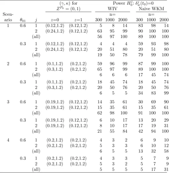
3.1 Simulation scenarios for T(Z) forZP0 in presence of competing
risks (J = 2) and power of a size α = 0.05 WIV test of H0 :
δw(j t0) = 0 and the naive WKM test discussed in Section 3.4 for
n= 300,1000,2000. Results are based on θ = ([1−θ01]/2, θ01,
0, [1−θ01]/2) for variousθ01. The hazard for eachj within each
ZP0 has Weibull hazard of the form κγ(γt)κ−1 for parameters
(γ, κ). For ZP0 = (1,1), (γ, κ) = (0.10,1) for j = 1,2 and for
ZP0 = (0,0), (γ, κ) = (0.16,1) for j= 1,2. . . . . 72
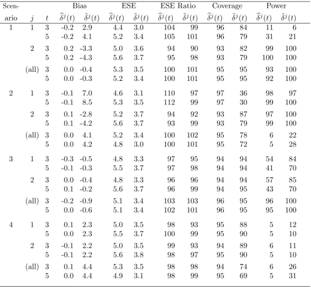
3.2 Simulation results: bias (×100), empirical standard error (ESE) (× 100), the ratio of the average estimated standard error and the empirical standard error (ESE Ratio, %), coverage of point-wise 95% confidence intervals forδj(t) and the percent power to rejectH0j(t) : δj(t) = 0 (%) based on (i) the IV estimators and pointwise confidence intervals and (ii) the naive estimators and confidence intervals for simulation Scenarios 1–4 as described in
Table 3.1 forθ01= 0.6 andn= 1000. . . 73
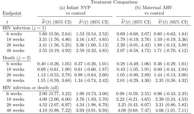
3.3 Results for the BAN study: IV ˆδj(t) and naive ˜δj(t) estimates (×100) and corresponding 95% confidence intervals for (a) infant NVP versus control and (b) maternal ARV versus control and for endpoints of infant HIV infection (j= 1), death (j= 2) and
HIV infection or death (allj). . . 74
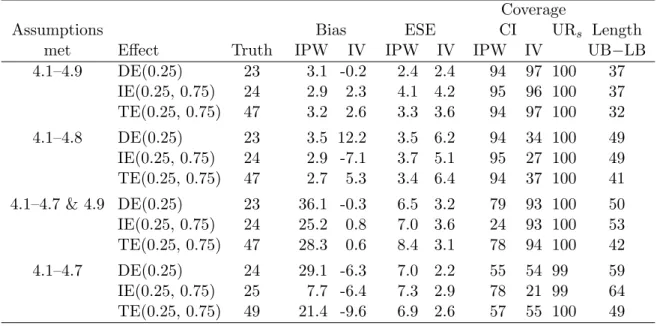
4.1 Simulation study results: true effect (×100), bias (×100), em-pirical standard error (ESE,×100), coverage of confidence inter-vals and strong uncertainty regions (%) for the estimators based on µIP W(z, α), µIV(z, α) and the lower (LB) and upper (UB)
bounds in 4.4 and 4.5 as well as the length of the bounds. . . 91 4.2 Group level characteristics: rural-urban continuum code of the
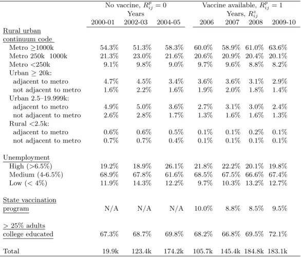
county; high, medium or low unemployment in the county (in the year 2006); whether or not there was a state funded vaccina-tion program and whether or not >25% of adults completed a college education (variablesVi) by enrollment year of the infants extracted from the MarketScan Research Databases and followed for rotavirus or acute gastroenteritis hospitalization (936,410
LIST OF FIGURES
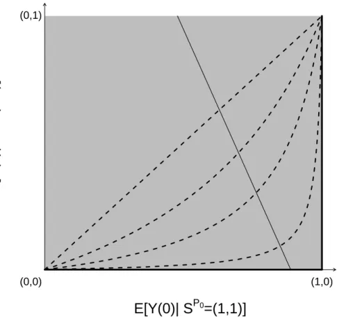
2.1 Graphical depiction of the bounds and sensitivity analysis model described in Sections 2.3.3 – 2.3.4. The solid thin line with neg-ative slope represents a set of joint distribution functions of (Z, S(1), S(0), Y(1), Y(0)) that all give rise to the same distribution of the observable random variables (Z, S, Y). The four dotted curves depict the log odds ratio selection model forγ = 0,1,2,4. The γ = 0 model is equivalent to the no selection model. Each selection model identifies exactly one pair of expectations from this set, rendering the principal effect (2.10) identifiable. The thick black lines on the edge of the unit square correspond to
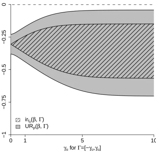
the lower bound of the principal effect. . . 54 2.2 Estimated ignorance regions irf0(β,Γ) and 95% pointwise
un-certainty regions URp(β,Γ) for the pertussis vaccine example in Section 2.7.3. The principal effect (2.10) is denoted β and Γ = [−γu, γu] for γu along the horizontal axis. The curve given by the lower boundary of the area with black slanted lines corre-sponds to ˆβl, the minimum of the estimated ignorance regions, and the upper bound of the area with black slanted lines cor-responds to ˆβu, the maximum of the estimated ignorance re-gion. The curve given by the lower (upper) boundary of the gray shaded area corresponds to the minimum (maximum) of
the 95% pointwise uncertainty region. . . 55
3.1 Application to the BAN study: cumulative incidence estimates partitioned by cause and results of the hypothesis tests of no treatment effect on cumulative incidence of HIV,H01:δw1(t0) = 0;
no treatment effect on death, H01: δw2(t0) = 0; and no effect of
treatment on death or cumulative incidence of HIV,H0:δw(t0) =
0 based on the WIV tests in Proposition 3.2 for (a) infant NVP
versus control and (b) maternal ARV versus control. . . 75
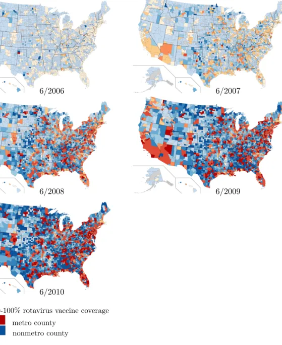
4.1 Map of the US counties estimated rotavirus vaccine coverage by study year as indicated by color. Deepening shades indicate higher vaccine coverage as indicated by the legend. Orange or red shaded counties indicate a metropolitan county (100,000 or more individuals) and blue shaded counties are nonmetropolitan (source: United States Department of Agriculture, Economic Research Service from the 2010 US census). Grey shaded areas indicate that no infants were enrolled in the study for that county
4.2 Estimates of DE(α), IE(0, α) and TE(0, α) for variousαbased on µIP W(z, α) (solid lines),µIV(z, α) (dotted lines) and the bounds based on µLB(z, α) and µU B(z, α) (shaded area) for the AGE
CHAPTER 1: INTRODUCTION AND LITERATURE REVIEW
1.1 Introduction
The goal of many health and epidemiological studies is to gain insight into the mechanisms that cause disease or other health outcomes and then use that insight to prevent disease and/or better health outcomes. These mechanisms may consist of one or more causal pathways in which different exposure states or risk factors lead to various effects (Rothman, 1976). Epidemiological studies often seek to investigate not only whether or not various sets of exposures or risk factors are on any of the causal pathways to a health outcome of interestY but also the size and nature of the effects of these exposures on this causal pathway.
1.1.1 The Potential Outcomes Model
Using the potential outcomes approach from Rubin (1974), letzdenote the various levels of the exposure or factor for which causal comparisons are being drawn, andZ the observed value of the exposure z which is observed prior to the outcome of interest Y. The potential outcome Y(z) is defined as the value of the outcome under exposure status z; for example, z might be a medical intervention or treatment with z= 1 denoting treatment received and z = 0 denoting control or treatment not received. The potential outcome Y(1) would then be the outcome had treatmentz = 1 been received and Y(0) the outcome had control been received.
Causal effects at the unit level can be defined as some function of the potential outcomes Y(z) that compare different levels of the exposurez. In order to define sensible causal effects each level of the exposure in the effect must be able to be observed in the units under study. For example, an individual causal treatment effect might be defined as the difference between an individual’s outcome under treatment compared to control, Y(1) − Y(0), which is not well defined if it is not possible for an individual or unit to experience both z = 0 and z= 1 (Holland, 1986). Often the target of inference in health and epidemiological studies is some population level parameter or population level causal effect such as the mean difference between the potential outcomes under treatment and control, E[Y(1]−Y(0)] or average treatment effect (ATE). HereE[Y(1)] is the mean potential outcome of the target population if everyone were treated (Z = 1), and E[Y(0)] the mean potential outcome if no one were treated (Z= 0).
exposureZ. This assumption has been referred to as a consistency assumption in the litera-ture (Cole and Frangakis, 2009) and will be termed causal consistency here to avoid confusion with concepts of statistical consistency. With this assumption, one potential outcome for each individual is observed and known, but the potential outcomes Y(z0) for Z 6= z0 are termed counterfactual and are unobserved. A third basic assumption frequently made in studying causal effects is that the exposure of one unit under study does effect the outcomes of other individuals or units, this is referred to as an assumption of no interference between units. Collectively these three assumptions are often referred to as the stable unit treatment value assumption or SUTVA (Rubin, 1980).
The assumptions contained in SUTVA will be reasonable in many situations, but unfor-tunately are not strong enough to allow for estimation of most population level causal effects such as the average treatment effect, E[Y(1)−Y(0)]. Under SUTVA, the observation of Y and Z for some population of units allows us to estimate E[Y(z)|Z = z], thus allowing for estimation of the associational effect
E[Y(1)|Z = 1]−E[Y(0)|Z = 0], (1.1)
but estimation of the ATE, a causal effect, is not possible without further assumptions. Under experimental settings the observed exposure or treatmentZ might be under the control of the experimenter and random assignment of Z to the units under study would give plausibility to the assumption that
Y(z)qZ forz= 0,1 (1.2)
can be accomplished then (1.2) might be replaced by
Y(z)qZ|X forz= 0,1, (1.3)
which will be plausible if all factors that confound the causal effect of Z on Y are measured inX. Under (1.3) the ATE may be consistently estimated using by weighting by the inverse probability of exposurez
E[Y(1)|Z = 1;X] Pr[Z = 1|X] −
E[Y(0)|Z = 0;X]
Pr[Z = 0|X] (1.4)
which is a function of associational parameters that may be consistently estimated from the data. Estimators based on (1.4) are referred to as inverse probability of treatment weighted estimators.
1.1.2 Instrumental Variables
Measuring all factors X such that (1.3) holds is one of the biggest challenges of causal inference in epidemiological research, particularly because it is not possible to provide evidence that (1.3) holds using empirical statistical tests. If there are factors U not measured in X that confound the effect of Z on Y(z) then the resulting inverse probability estimators will be biased. A method to potentially avoid this problem of unmeasured confounding entails the use of instrumental variables. A variable R is considered an instrumental variable if it meets the following three criteria: i)Rhas a causal effect on the exposure of interestZ, ii)R affects the outcomeY only through its effect onZ and iii)R does not share common causes withY (Hern´an and Robins, 2006).
of the two potential values ofZ(r),SP0= (Z(0), Z(1)), stratification of the potential outcomes
Y(z) bySP0 is commonly referred to as principal stratification (Frangakis and Rubin, 2002).
A local average treatment effect or principle effect is the average treatment effect in one of the strata defined bySP0, where causal effects in the strata defined bySP0 = (0,1) are commonly
of interest. Imbens and Angrist (1994) showed the local average treatment effect (LATE) defined as E[Y(1)−Y(0)|SP0 = (0,1)] is identifiable under four assumptions: independent
treatment instrument
Rq {Y(z), Z(r)} forz.r= 0,1, (1.5)
monotonicity with respect toZ
Pr[Z(1)≥Z(0)] = 1, (1.6)
exclusion restriction
Y(0) =Y(1) ifZ(0) =Z(1), (1.7)
and if there is a nonzero causal effect ofR on Z, namely
E[Z(1)−Z(0)]6= 0. (1.8)
The monotonicity assumption (2.21) states there are no individuals such that Z(0) = 1 and Z(1) = 0, meaning that the principal strata SP0 = (1,0) is empty. Assumption (1.7) states
that Z has no effect on Y in individuals who are always exposed SP0 = (1,1) or are never
exposed SP0 = (0,0). Assumption (1.8) indicates that the instrument R has a causal effect
on the exposureZ. Under these four assumptions the LATE can be expressed as
E[Y|R= 1]−E[Y|R = 0]
E[Z|R= 1]−E[Z|R= 0]. (1.9)
E[Y(1)−Y(0)|SP0 = (0,1)] equals (1.9), first note under the assumptions that the numerator
of (1.9) equals E[Y(1)−Y(0)] = E[{Y(1)−Y(0)}{Z(1)−Z(0)}] = E[Y(1)−Y(0)|Z(1) > Z(0)] Pr[Z(1)> Z(0)]. Similarly, the denominator of (1.9) equals Pr[Z(1) = 1]−Pr[Z(0) = 1] = Pr[Z(0) = 0, Z(1) = 1] = Pr[Z(1)> Z(0)], which is non-zero under (1.8).
Obtaining a valid instrument such that (1.5–1.8) hold can prove to be a difficult task. An example of a variable R that might satisfy (i)-(iii) such that (1.5–1.8) hold is the calendar time for the FDA approval of a novel treatment for a disease, where here Z would be the novel treatment. Let R = 1 denote that diagnosis of the disease was after the calendar time for the approval of the new treatment, and R = 0 indicate diagnosis was before this calendar time; letZ = 1 denote that the novel treatment was selected and Z = 0 denote that treatment was not selected. The principal strata vector would indicate a subject’s treatment selection before and after the calendar time FDA approval for the novel treatment, for instance SP0 = (1,1) would be represent individuals that would take the treatment regardless of the
FDA calendar time approval. In this situation Y might represent survival to a given time point after having been diagnosed with the disease, thus the local average treatment defined as E[Y(1)−Y(0)|SP0 = (0,1)] would represent the difference in the proportion surviving
serum cholesterol and cancer might use a genetic determinant of serum cholesterol as the instrumental variable (Martens et al., 2006).
1.1.3 Interference
When studying causal effects of a treatment or exposure, sometimes the treatment or exposure received by one individual may affect the outcomes of other individuals under study. In the causal inference literature this is referred to as interference and is most frequently encountered in settings in which outcomes are largely dependent on social happenings. Some well known examples of settings where this might occur include the study of infectious diseases and vaccination, educational interventions and effects of housing voucher programmes. Until recently most of the causal inference literature has operated under the assumption that there is no interference between units (Cox, 1958, this assumption is included in SUTVA). In the aforementioned settings this assumption is not only undoubtedly violated, but the pattern of interference between units is often a target of inference useful in determining important social and public health policies.
Though most of the causal inference literature operates under the assumption of no in-terference, Rubin (1980) noted that the potential outcomes framework could be extended to accommodate interference between units. Specifically, assume that there are N > 1 groups or communities for which data are observed, with each group having ni individuals for i = 1, . . . , N. Let Zi = (Zi1, . . . , Zini) denote the treatment selections or exposures of those ni individuals for each group i. Assume that Zij is a dichotomous, taking values 0 for no exposure or treatment not selected, and 1 for exposure or treatment selected. Let Zi,−j = (Zi1, . . . Zij−1, Zij+1, . . . , Zini) denote the ni−1 subvector of treatment selections for group i with entry j deleted. Define Z(ni) as the set of possible treatment selections for a group of sizeni. Zi,−j takes on values in the setZ(ni−1). There are 2ni different realizations of the vector Zi, and 2ni−1 realizations of Zi,−
ith group for treatment allocation vector Zi by Yij(Zi). Denote the potential outcomes for all members of groupiasYi(Zi). This allows for interference between members of the same group, but does not allow for interference between members of different groups. This is an assumption, and is referred to as partial interference in the literature. In Manski (2013) this assumption is a specific case of a more general class of assumptions which he calls constant treatment response assumptions (CTR). This assumption is reasonable if interaction between members of different groups is minimal or nonexistent.
Halloran and Struchiner (1995) took Rubin’s suggestion and defined several new causal ef-fects unique to studying interference: direct, indirect, total and overall efef-fects. The individual direct, indirect, total and overall effects are defined as
DEij(zi,−j) =Yij(zi,−j, zij = 0)−Yij(zi,−j, zij = 1), IEij(zi,−j,zi,0−j) =Yij(zi,−j, zij = 0)−Yij(zi,0−j, zij = 0), T Eij(zi,−j,zi,0−j) =Yij(zi,−j, zij = 0)−Yij(zi,0−j, zij = 1), and
OEij(zi,zi0) =Yij(zi)−Yij(zi0).
The direct effect compares potential outcomes that keep the treatment of other members of the same group constant and comparing the effect of treatment in the individual. The indirect effect compares two different treatment allocation vectors given to other members of the group while holding the treatment given to the individual constant atzij = 0. The total effect compares both the different treatment allocation vectors and the effect of treatment in the individual. The overall effect compares any two treatment allocation vectors for the whole group and may correspond to a direct effect, indirect effect or a total effect, or another effect.
Often it is still of interest to compare 2 specific treatment allocation strategies or laws, denotedπi(Zi, α0) andπi(Zi, α1), say for example comparing causal effects when vaccinating
1/3 of the population versus vaccinating 2/3 thirds of the population. The parametersα0 and
For the purposes here, a Bernoulli type parametrization ofπi(Zi, α0) will be assumed:
πi(Zi, α0) =
ni
Y
j=1
αZij
0 (1−α0)1−Zij (1.10)
Sobel (2006) introduced the idea of defining causal estimands that average over all possible treatment assignment vectors according to some treatment allocation law in a paper assessing the comparative effectiveness of different housing voucher programmes. Specifically, let
Yij(z, α0) =
X
s∈Z(ni−1)
Yij(zi,−j =s, zij =z)Prα0(Zi,−j =s|Zij =z)
and
Yij(α0) =
X
s∈Z(ni)
Yij(zi=s)πi(Zi,j =s;α0);
then the individual average direct, indirect, total and overall effects are defined as
DEij(α0) =Yij(0;α0)−Yij(1;α0),
IEij(α0, α1) =Yij(0;α0)−Yij(0;α1),
T Eij(α0, α1) =Yij(0;α0)−Yij(1;α1),
OEij(α0, α1) =Yij(α0)−Yij(α1).
Now the direct effect compares the effect of treatment in individual ij while holding the treatment allocation strategy constant, the indirect effect compares the effect of the treatment allocation strategy constant while holding the treatment to the individual constant atzij = 0. The total effect compares both the treatment allocation strategies and treatment given to individual ij. Group average direct, indirect, total and overall effects can be defined by taking the mean for group i of DEij(α0), IEij(α0, α1), T Eij(α0, α1) and OEij(α0, α1) (i.e.
DEi(α0) =
ni
P
j=1
DEij(α0) and so forth). Population average direct, indirect, total and overall
effects can be defined by taking the mean of the group average direct, indirect, total and overall effects (i.e. DE(α0) =
N
P
i=1
The so called gold standard for achieving accurate estimates of causal estimands compar-ing these two allocation strategies is 2-stage randomization, where both individual treatment assignment is randomized as well as treatment allocation strategy to various groups or com-munities. The majority of the inferential methods developed for the population average direct, indirect, total and overall effects rely on the assumption that there are two levels of randomization. Rosenbaum (2007) developed nonparametric inferential methods for assessing treatment effects in presence of interference under 2 stage randomized treatment assignment. Hudgens and Halloran (2008) formalized the definitions of direct, indirect, total and overall effects averaged over all possible treatment assignment vectors and developed unbiased es-timators and corresponding variance upper bounds for these causal treatment effects under 2 stage randomization and an additional assumption referred to as stratified interference. Stratified interference assumes
Yij(zi,−j, zij) =Yij(zi,0−j, zij) for
X
j zij =
X
j zij0 .
which means that potential outcomes will remain constant when the same number of other members of the group are treated and treatment to the individual remains constant. This reduces the number of potential outcomes for each individual from 2ni ton
i. Tchetgen Tch-etgen and Vanderweele (2012) improved upon the variance bounds developed by Hudgens and Halloran (2008) for these effects under 2 stage randomization by relaxing the stratified interference assumption.
Hong and Raudenbush (2006) consider interference effects in the context of educational performance. In this setting randomization is not present at either the individual level or the group level. The independent treatment assignment assumption that 2 stage randomization makes plausible
{Y(zi)}z
i∈Z(ni)qZi
fori= 1, . . . , N is replaced by
{Y(zi)}z
for some set of covariatesXi. Tchetgen Tchetgen and Vanderweele (2012) derived the follow-ing inverse probability of treatment weighted estimators forYi(z, α0)] (the group average) to
be used for inference of the population average direct, indirect, and total effects
b
YiIP W(z, α0) =
Pni
j=1πi(Zi,−j;α0)Yij(Zi)I[Zij =z]
nifZ|X,i(Zi|Xi)
for a the Bernoulli type parametrization ofπ(Zi, α0) given above and wherefZ|X,i(zi|Xi) = Pr[Zi = zi] is the estimated probability of treatment allocation vector Xi given covariates Xi. Tchetgen Tchetgen and Vanderweele (2012) suggest using a logistic-normal mixed effects model to estimatefZ|X,i(Zi|Xi).
Though the advancements made account for interference and allow for definition of causal effects specific to interference, many of the results obtained are limited by the need for 2 stage randomized designs requiring randomization at the individual level within each group, as well as randomization of groups to different treatment allocation strategies. Such designs are difficult, all but infeasible to implement in practice, thus there is a strong need for adap-tations to be used for observational data or for randomized designs not necessarily having achieving randomization at both the group and the individual level. Both Hong and Rau-denbush (2006) and Tchetgen Tchetgen and Vanderweele (2012) have obtained results for observational data under the assumption that conditional on measured covariates, treatment assignment is independent of the potential outcomes. Hong and Raudenbush (2006) devel-oped results for estimators of interference effects within strata defined by different levels of Xi and Tchetgen Tchetgen and Vanderweele (2012) derived inverse probability of treatment weighted estimators of interference effects. Both the results of Hong and Raudenbush (2006) and Tchetgen Tchetgen and Vanderweele (2012) enjoy the same results obtained under 2 stage randomization in terms of inference, but are limited by the fact that they rely on a strong conditional independent treatment assignment assumption and require measurement of all covariates required for conditional independence of the treatment and potential outcomes.
CHAPTER 2: NONPARAMETRIC BOUNDS AND SENSITIVITY ANALYSIS OF TREATMENT EFFECTS
2.1 Introduction
In many areas of science, interest often lies in assessing the causal effect of a treatment (or exposure) on some particular outcome of interest. For example, researchers may be interested in estimating the difference between the average outcomes when all individuals are treated (exposed) versus when all individuals are not treated (unexposed). When treatment is assigned randomly and there is perfect compliance to treatment assignment, such treatment effects are identifiable and inference about the effect of treatment proceeds in a straightforward fashion. On the other hand, if the treatment assignment mechanism is not known to the analyst or compliance is not perfect, then these treatment effects are not identifiable from the observable data.
identifi-ability also arises when drawing inference about treatment effects within principal strata or effects describing relationships between an outcome and a treatment that are mediated by some intermediate variable.
In order to conduct inference about treatment effects that are partially identifiable, two approaches are often employed: (i) bounds are derived for the treatment effect under minimal assumptions, or (ii) additional untestable assumptions are invoked under which the treat-ment effect is identifiable and then sensitivity analysis is conducted to assess how inference about the treatment effect changes as the untestable assumptions are varied. Below (i) and (ii) are illustrated in five settings. In Section 2.2 we consider treatment effect bounds and sensitivity analysis when the treatment assignment mechanism is unknown. In Section 2.3 partial identifiability of principal strata causal effects are discussed. In Section 2.4 the setting of non-compliance is considered where there is interest in assessing the effect of treatment if there was perfect compliance. In Section 2.5 bounds and sensitivity analysis for direct and indirect effects in mediation analysis are presented, and in Section 2.6 longitudinal treatment effects are considered. Much of the literature on bounds and sensitivity analysis focuses on ignorance due to partial identifiability and tends to ignore uncertainty due to sampling er-ror. Section 2.7 presents some methods that appropriately quantify this uncertainty when drawing inference about partially identifiable treatment effects. Section 2.8 concludes with a discussion.
2.2 Treatment Selection
2.2.1 Minimal Assumptions Bounds
Throughout this paper we invoke the stable unit treatment value assumption (SUTVA; Rubin, 1980), i.e., there is no interference between units and there are no hidden (unrepresented) forms of treatment such that each individual has two potential outcomes {Y(0), Y(1)}. The no hidden forms of treatment guarantees that the observed outcome is equal to the potential outcome corresponding to the observed treatment, namely that Y = Y(z) for Z = z. Here this will be referred to as the causal consistency assumption; for further discussion of causal consistency see Pearl (2010) and references therein. Once an individual receives treatmentZ, the potential outcomeY(Z) is observed and the other potential outcome (or counterfactual) Y(1−Z) becomes missing. Assume that niid copies of (Z, Y) are observed and denoted by (Zi, Yi) for i= 1, . . . , n.
In this section we consider treatment effect bounds when the treatment assignment mech-anism is unknown. HereZ can be thought of as treatment selection by the individual or by nature, rather than random treatment assignment as in an experiment. Define the average treatment effect ATE to beE[Y(1)−Y(0)] =E[Y(1)]−E[Y(0)] whereEdenotes the expected value. The ATE can be decomposed as
1
X
z=0
E[Y(1)|Z =z] Pr[Z=z]− 1
X
z=0
E[Y(0)|Z =z] Pr[Z =z]. (2.1)
Note E[Y(z)|Z = z] = E[Y|Z = z] by the causal consistency assumption. Thus from the observed dataE[Y(z)|Z =z] and Pr[Z =z] are identifiable and can be consistently estimated by their empirical counterparts. On the other hand, the observed data provide no information about E[Y(z)|Z = 1−z], such that (2.1) is only partially identifiable without additional assumptions.
by settingE[Y(1)|Z = 0] = 0 and E[Y(0)|Z = 1] = 1, which yields the lower bound
E[Y(1)|Z = 1] Pr[Z = 1]−E[Y(0)|Z = 0] Pr[Z= 0]−Pr[Z= 1]. (2.2)
Similarly E[Y(1)−Y(0)] is bounded above by setting E[Y(1)|Z = 0] = 1 and E[Y(0)|Z = 1] = 0, which yields the upper bound
E[Y(1)|Z = 1] Pr[Z = 1]−E[Y(0)|Z = 0] Pr[Z= 0] + Pr[Z= 0]. (2.3)
These bounds were derived independently by Robins (1989) and Manski (1990). The lower and upper bounds (2.2) and (2.3) are sharp in the sense that it is not possible to derive narrower bounds without additional assumptions. Note the interval formed by (2.2) and (2.3) is contained in [−1,1] and is of width 1. Thus the bounds are informative in that the treatment effect is now restricted to half of the otherwise possible range [−1,1]. On the other hand, the bounds will always contain the null value 0 corresponding to no average treatment effect. That is, without additional assumptions the sign of the treatment effect cannot be determined from the observable data.
2.2.2 Additional Assumptions
An example of an additional assumption is mean independence, i.e.,
E[Y(z)|Z = 0] =E[Y(z)|Z = 1] for z= 0,1. (2.4)
Under (2.4) ATE is identifiable. Specifically the upper and lower bounds (2.2) and (2.3) both equalE[Y(1)|Z = 1]−E[Y(0)|Z = 0], which is identifiable from the observable data and can be consistently estimated by the “naive” estimator given by the difference in sample means between the groups of individuals receiving treatment and control. Assumption (2.4) will hold in experiments where treatment is randomly assigned as in a randomized clinical trial. Moreover, in randomized experiments the stronger assumption
Y(z)qZ forz= 0,1, (2.5)
will hold, which in turn implies (2.4).
In some settings it may be reasonable to consider additional assumptions that are not as strong as (2.4) or (2.5) but nonetheless lead to tighter bounds than (2.2) and (2.3). For example, monotonicity type assumptions might be considered, such as monotone treatment selection (MTS)
E[Y(z)|Z = 1]≥E[Y(z)|Z = 0] for z= 0,1. (2.6)
MTS assumes individuals who select treatment will on average have outcomes greater than or equal to that of individuals who do not select treatment under the counterfactual scenario all individuals selected the samez. Manski and Pepper (2000) consider MTS when examining the effect of returning to school on wages later in life. For this example, MTS implies individuals who choose to return to school will have higher wages on average compared to individuals who choose to not return to school under the counterfactual scenario no individuals return to school. Alternatively, one might assume monotone treatment response (MTR)
(Manski, 1997). MTR assumes that under treatment each individual will have a response greater than or equal to that under control. For instance, supposeZ = 1 if an individual elects to get the annual influenza vaccine and Z = 0 otherwise, and let Y(z) = 1 if an individual subsequently does not develop flu-like symptoms whenZ =z, andY(z) = 0 otherwise. MTR asserts that each individual is more or as likely to not develop flu-like symptoms if they are vaccinated versus if they are unvaccinated. Given to date there is no evidence that the annual flu vaccine enhances the probability of acquiring influenza, MTR might be plausible for this example.
Assuming MTS or MTR can lead to narrower bounds than (2.2) and (2.3) because they imply additional constraints on unobserved counterfactual expectations. For example, assum-ing MTS,E[Y(0)|Z = 1] is bounded below byE[Y(0)|Z = 0] and E[Y(1)|Z = 0] is bounded above byE[Y(1)|Z = 1], implying the upper bound on E[Y(1)−Y(0)] is
E[Y(1)|Z = 1]−E[Y(0)|Z = 0], (2.7)
for which the naive estimator is consistent. Under MTS the lower bound remains (2.2). In contrast to the no assumptions bounds, assuming MTS the bounds may exclude 0, specifically when (2.7) is negative. MTR impliesE[Y(1)] ≥E[Y(0)] which in turn implies that the ATE lower bound is 0. Under MTR the upper bound remains (2.3).
2.2.3 AZT Example
empirical estimates of the no assumptions bounds (2.2) and (2.3) equal−0.7 and 0.3. In this setting, the MTS assumption (2.6) supposes that individuals who elected to take AZT would have been more or as likely to die as individuals who did not take AZT in the counterfactual scenarios where everyone receives treatment or everyone does not receive treatment. This might be reasonable if it is thought that those who took AZT were on average less healthy than those who did not. Assuming MTS, the upper bound (2.7) is estimated to be -0.48. Thus in this example the MTS bounds are substantially tighter than the no assumption bounds. The estimated MTS bounds lead to the conclusion (ignoring sampling variability, a point which we return to later) that AZT reduces the probability of death by at least 0.48 whereas without the MTS assumption we cannot even conclude whether the effect of treatment is non-zero.
2.2.4 Sensitivity Analysis
Assumptions such as (2.4) or (2.5) which identify the ATE, or assumptions such as MTS which sharpen the bounds, cannot be tested empirically because such assumptions pertain to the counterfactual distribution of Y(z) given Z = 1−z. Robins and others (e.g., see Robins et al., 1999; Scharfstein et al., 1999) have argued that a data analyst should conduct sensitivity analysis to explore how inference varies as a function of departures from any untestable assumptions.
least as strongly associated with lung cancer as cigarette use. This idea was further developed by Schlesselman (1978); Rosenbaum and Rubin (1983); Lin et al. (1998); Hern´an and Robins (1999); and VanderWeele and Arah (2011) among others.
To illustrate this approach, suppose in the AZT example above that the analyst first assumes (2.5) holds and thus estimates the effect of AZT to be -0.48. To proceed with sensitivity analysis, the analyst posits the existence of an unmeasured binary variableU and assumes thatY(z)qZ|U forz= 0,1. Similar to VanderWeele and Arah (2011), let
c(z) ={E[Y(z)|U = 1]−E[Y(z)|U = 0]}{Pr[U = 1|Z =z]−Pr[U = 1]}.
Then under the assumption that Y(z)qZ|U for z = 0,1, the naive estimator converges in probability to E[Y(1)]−E[Y(0)] +c(1)−c(0). Thus the naive estimator is asymptotically unbiased if and only if c(1) =c(0). For an alternative decomposition of the asymptotic bias of the naive estimator see Morgan and Winship (2007,§2.6.3)
Sensitivity analysis proceeds by making varying assumptions about the unidentifiable associations of U with Y(0), Y(1), and Z. Under the most extreme of these assumptions the bounds (2.2) and (2.3) are recovered. In particular, the upper bound in (2.3) is achieved when Pr[U = 1|Z = 1] = 0, Pr[U = 1|Z = 0] = 1,E[Y(1)|U = 1] = 1 andE[Y(0)|U = 0] = 0, meaning that the confounderU is perfectly negatively correlated with treatmentZ and that if the confounder is present (U = 1), then a treated individual will die, whereas if the confounder is absent (U = 0), then an untreated individual will survive. The lower bound (2.2) is achieved under the opposite conditions.
instance, suppose the analyst further assumes that E[Y(z)|U = 1] − E[Y(z)|U = 0] does not depend on z. This assumption will hold if the effect of Z on Y is the same if U = 0 or U = 1. Letting γ0 = E[Y(z)|U = 1] − E[Y(z)|U = 0] and γ1 = Pr[U = 1|Z = 1] −
Pr[U = 1|Z = 0], the asymptotic bias of the naive estimator is then given by γ0γ1 and a bias
adjusted estimator is found by subtractingγ0γ1 from the naive estimator. Sensitivity analysis
may proceed by determining the values ofγ0 and γ1 for which the bias adjusted estimator of
the ATE will have the opposite sign of the naive estimator. For the AZT example, the bias adjusted estimator will have the opposite sign of the naive estimator if γ0γ1 <−0.48. This
indicates that the product of (i) the difference in the mean potential outcomes between levels of the confounder for both treatment and control and (ii) the difference in the prevalence of the unmeasured confounder between the treatment and control groups must be less than -0.48. Such magnitudes might be considered unlikely in the opinion of subject matter experts, in which case the sensitivity analysis would support the existence of a beneficial effect of AZT on survival among HIV+ men (ignoring sampling variability). Note the observed data distribution places some restrictions on the possible values of (γ0, γ1), i.e., (γ0, γ1) is partially
identifiable. For instance, ifγ1= 1 then Pr[U = 1|Z = 1] = 1 and Pr[U = 1|Z = 0] = 0 which
impliesE[Y(z)|U =u] =E[Y(z)|Z =u] and therefore max{E[Y(1)|Z = 1]−1,−E[Y(0)|Z = 0]} ≤ γ0 ≤ min{E[Y(1)|Z = 1],1−E[Y(0)|Z = 0]}. Such considerations should be taken
into account when determining the range of values of (γ0,γ1) in sensitivity analysis.
Because the data provide no evidence about U, VanderWeele (2008) and VanderWeele and Arah (2011) recommend choosing U and any simplifying assumptions based on what is considered plausible by relevant subject-matter experts. Such sensitivity analyses are most applicable when the existence of unmeasured confounders is known, but these factors could not be measured for logistical or other reasons. General bias formulas to be used for sensitivity analyses of unmeasured confounding for categorical or continuous outcomes, confounders, and treatments can be found in VanderWeele and Arah (2011).
analysis strategy described above would not be applicable or feasible. One general alternative approach entails making additional untestable assumptions regarding the unobserved poten-tial outcome distributions. Typically these assumptions (or models) are indexed by one or more sensitivity analysis parameters conditional upon which the causal estimand of interest is identifiable (e.g., Scharfstein et al., 1999; Brumback et al., 2004). Sensitivity analysis then proceeds by examining how inference changes as assumed values of the parameters are varied over plausible ranges. Examples of such sensitivity analyses are given below in Sections 2.3.4 and 2.6.3.
2.2.5 Covariate Adjustment
Typically in observational studies baseline (pre-treatment) covariates X will be collected in addition toZandY. Incorporating information from observed covariates can help sharpen inferences about partially identified treatment effects. For example, incorporating covariates will generally lead to narrower bounds (Scharfstein et al., 1999). This follows because any treatment effect consistent with the distribution of observed variables (X, Y, Z) must also be consistent with the distribution of (Y, Z), i.e., the observable variables if we do not observe or choose to ignoreX (Lee, 2009). Covariate adjusted bounds are discussed further in Section 2.3.3 below.
Additionally, incorporating covariates may lend plausibility to some of the bounding as-sumptions discussed in Section 2.2.2. For example, in the absence of randomized treatment assignment (2.4) or (2.5) may be dubious. Instead of (2.4) it might be more plausible to assume
E[Y(z)|Z = 0, X =x] =E[Y(z)|Z = 1, X=x] forz= 0,1. (2.8)
Similarly, assumption (2.5) might be replaced by
Y(z)qZ|X forz= 0,1, (2.9)
of covariates. Assumption (2.9) is commonly referred to as no unmeasured confounders. Assumptions such as (2.8) or weaker inequalities similar to (2.6) such as
E[Y(z)|Z = 1, X =x]≥E[Y(z)|Z = 0, X=x] forz= 0,1,
may be deemed plausible for certain levels ofX, but not for others. Availability of covariates also allows for the consideration of new types of assumptions (e.g., see Chiburis, 2010).
To conduct covariate adjusted sensitivity analysis, departures from identifying assump-tions such as (2.9) can be explored. Similar to the previous section, a departure from (2.9) might entail positing the existence of an unmeasured variable U associated with both treat-ment selection Z and the potential outcomes Y(z) for z = 0,1. Under this scenario, one might postulate thatY(z)qZ|{X, U} forz= 0,1 rather than (2.9) and sensitivity analysis proceeds by examining how inference varies as a function of the magnitude of the association of U with Z,Y(0), and Y(1) givenX. Similar to covariate adjusted bounds, smaller associ-ations or tighter regions of the values of the sensitivity parameters may be deemed plausible within certain levels ofX, potentially yielding sharper inferences from the sensitivity analy-ses. However, as cautioned by Robins (2002), care should be taken in clearly communicating the meaning of such sensitivity parameters and their relationship to covariates when eliciting plausible ranges from subject matter experts. In some scenarios plausible regions for sensi-tivity parameters may in fact be wider when conditioning onX than when not conditioning onX.
2.3 Principal Stratification
2.3.1 Background
some individuals die, investigators might be interested in treatment effects only among indi-viduals alive at the end of the study. Unfortunately, estimands defined by contrasting mean outcomes under treatment and control that simply condition on this observable intermediate variable do not measure a causal effect of treatment without additional assumptions. One approach that may be employed in this scenario entails principal stratification (Frangakis and Rubin, 2002). Principal stratification uses the potential outcomes of the intermediate post-randomization variable to define strata of individuals. Because these “principal strata” are not affected by treatment assignment, treatment effect estimands defined within princi-pal strata have a causal interpretation and do not suffer from the complications of standard post-randomization adjusted estimands. The simple framework of principal stratification has a wide range of applications. For a recent discussion of the utility (and lack thereof) of principal stratification, see Pearl (2011) and corresponding reader reactions.
As a motivating example for this section, we consider evaluating vaccine effects on post-infection outcomes. In vaccine studies, uninfected subjects are enrolled and followed for infection endpoints, and infected subjects are subsequently followed for post-infection out-comes such as disease severity or death due to infection with the pathogen targeted by the vaccine; often interest is in assessing the effect of vaccination on these post-infection endpoints (Hudgens and Halloran, 2006). For example, Preziosi and Halloran (2003) present data from a pertussis vaccine field study in Niakhar, Senegal. In this study 3845 vaccinated children and 1020 unvaccinated children were followed for one year for pertussis. In the vaccine group 548 children contracted pertussis, of whom 176 had severe infections; in the unvaccinated group 206 children contracted pertussis, of whom 129 had severe infections. In this setting investi-gators are interested in assessing whether or not the vaccine had an effect on the severity of infection.
an approach does not distinguish vaccine effects on susceptibility to infection from effects on the post-infection endpoint of interest. An analysis that conditions on infection attempts to distinguish these effects and may be more sensitive in detecting post-infection vaccine effects. However, because the set of individuals who would become infected under control are not likely to be the same as those who would become infected if given the vaccine, conditioning on infection might result in selection bias. For example, those who would become infected un-der vaccine may tend to have weaker immune systems than those who would become infected under control, and thus are more susceptible to severe infection. Because of this potential selection bias, comparisons between infected vaccinees and infected controls do not necessarily have causal interpretations.
2.3.2 Principal Effects
In this section treatment is vaccination, with Z = 1 corresponding to vaccination and Z = 0 corresponding to not being vaccinated. Assume that assignment to vaccine is equivalent to receipt of vaccine, i.e., there is no non-compliance. Denote the potential infection outcome byS(z), whereS(z) = 0 if uninfected andS(z) = 1 if infected. Here the focus is on evaluating the causal effect of vaccine on Y, a post-infection outcome. For simplicity we consider the case where Y is binary, indicating the presence of severe disease. If S(z) = 1, define the potential post-infection outcome Y(z) = 1 if the individual would have the worse (or more severe) post-infection outcome of interest givenz, and Y(z) = 0 otherwise. If an individual’s potential infection outcome for treatment z is uninfected, (i.e., S(z) = 0), then we adopt the convention thatY(z) is undefined. In other words, it does not make sense to define the severity of an infection in an individual who is not infected. This convention is similar to that employed in other settings. For instance, in the analysis of quality of life studies it might be assumed that quality of life metrics are not well defined in those who are not alive (Rubin, 2000).
Define abasic principal stratificationP0according to the joint potential infection outcomes
joint potential infection outcomes, (S(0), S(1)), and are composed of immune (not infected under both vaccine and placebo), harmed (infected under vaccine but not placebo), protected (infected under placebo but not vaccine), and doomed individuals (infected under both vaccine and placebo). Note the only stratum where both potential post-infection endpoints are well defined is in the doomed basic principal stratum,SP0 = (1,1). Thus defining a post-infection
causal vaccine effect is only possible in the doomed principal stratum SP0 = (1,1). Such a
causal estimand will describe the effect of vaccination on disease severity in individuals who would become infected whether vaccinated or not. For instance, the vaccine effect on disease severity may be defined by
E[Y(1)|SP0 = (1,1)]−E[Y(0)|SP0 = (1,1)]. (2.10)
Frangakis and Rubin call treatment effect estimands such as (2.10) “principal effects.”
2.3.3 Bounds
Assume we observe n iid copies of (Z, S, Y) denoted by (Zi, Si, Yi) for i= 1, . . . , n. Also assume that the doomed principal strata is non-empty, Pr[SP0 = (1,1)] > 0, so that the
principal effect in (2.10) is well defined. Bounds for (2.10) are presented below under two additional assumptions: independent treatment assignment, i.e.,
Zq {Y(z), S(z)} forz= 0,1 (2.11)
and monotone treatment response with respect toS, i.e.,
Pr[S(0)≥S(1)] = 1. (2.12)
regarding Y. Under (2.11), assumption (2.12) implies P(S = 1|Z = 1) ≤P(S = 1|Z = 0), which is testable using the observed data. For the pertussis example, the proportion infected in the vaccine group was less than in the unvaccinated group; thus, assuming (2.11), the data do not provide evidence against (2.12).
Assuming independent treatment assignment and monotonicity, (2.10) is partially identi-fiable from the observable data. The left term of (2.10) can be written
E[Y(1)|SP0 = (1,1)] =E[Y(1)|S(1) = 1]
=E[Y(1)|S(1) = 1, Z = 1] =E[Y|S = 1, Z = 1],
(2.13)
where the first equality holds under (2.12), the second equality under (2.11), and the third by causal consistency. On the other hand, the right term of (2.10) is only partially identifiable. To see this, note
E[Y(0)|S(0) = 1] = E[Y(0)|SP0 = (1,1)] Pr[S(1) = 1|S(0) = 1]+
E[Y(0)|SP0 = (1,0)] Pr[S(1) = 0|S(0) = 1].
(2.14)
In (2.14), only E[Y(0)|S(0) = 1] and Pr[S(1) = s|S(0) = 1] for s = 0,1 are identifiable. In particular,E[Y(0)|S(0) = 1] =E[Y|S= 1, Z = 0] by similar reasoning to (2.13), and
Pr[S(1) = 1|S(0) = 1] = Pr[S(1) = 1] Pr[S(0) = 1] =
Pr[S = 1|Z = 1] Pr[S = 1|Z = 0],
where the first equality holds under (2.12) and the second under independent treatment as-signment (and causal consistency). The other two terms in (2.14), namely E[Y(0)|SP0 =
(1,1)] and E[Y(0)|SP0 = (1,0)], are only partially identifiable. In words, infected controls
E[Y(0)|SP0 = (1,1)] and hence (2.10).
For fixed values of E[Y(0)|S(0) = 1] and Pr[S(1) = 1|S(0) = 1], any pair of expectations (E[Y(0)|SP0 = (1,1)], E[Y(0)|SP0 = (1,0)])∈[0,1]2satisfying (2.14) will give rise to the same
observed data distribution. Equation (2.14) describes a line segment with non-positive slope intersecting the unit square as illustrated in Figure 1. An upper bound ofE[Y(0)|SP0 = (1,1)]
and thus a lower bound for (2.10) is achieved when the line intersects the right or lower side of the square, i.e., when either
E[Y(0)|SP0 = (1,1)] = 1 or E[Y(0)|SP0 = (1,0)] = 0. (2.15)
Together (2.14) and (2.15) implyE[Y(0)|SP0 = (1,1)] is bounded above by
min
1, E[Y(0)|S(0) = 1] Pr[S(1) = 1|S(0) = 1]
. (2.16)
Similarly, E[Y(0)|SP0 = (1,1)] is bounded below by
max
0,E[Y(0)|S(0) = 1]−Pr[S(1) = 0|S(0) = 1] Pr[S(1) = 1|S(0) = 1]
. (2.17)
Combining (2.17) with (2.13) yields the upper bound on the principal effect of interest (2.10) and combining (2.16) with (2.13) yields the lower bound. These bounds were derived by Rotnitzky and Jemiai (2003); Zhang and Rubin (2003); and Hudgens et al. (2003). Con-sistent estimates of (2.16) and (2.17) can be computed by replacing E[Y(0)|S(0) = 1] with
P
iYiI(Si = 1, Zi= 0)/PiI(Si = 1, Zi= 0) and Pr[S(1) = 1|S(0) = 1] with
min
1,
P
iI(Si =Zi = 1)/PiI(Zi= 1)
P
iI(Si = 1, Zi = 0)/
P
iI(Zi = 0)
.
Note if Pr[S(1) = 1|S(0) = 1] = 1, i.e., the vaccine has no protective effect against infection, then the protected principal stratum SP0 = (1,0) is empty and both (2.16) and
(2.17) equalE[Y(0)|S(0) = 1] meaning that (2.10) is identifiable and equals E[Y|Z = 1, S = 1]−E[Y|Z = 0, S = 1]. Intuitively the lack of vaccine effect against infection eliminates the potential for selection bias.
As discussed in Section 2.2.5, incorporation of covariates can tighten bounds. For covari-atesXwith finite support, one simple approach of adjusting for covariates entails determining bounds within strata defined by the levels of X and then taking a weighted average of the within strata bounds over the distribution ofX. For the bounds in (2.16) and (2.17), adjust-ment for covariates will always lead to bounds that are at least as tight as bounds unadjusted for covariates (Lee, 2009; Long and Hudgens, 2013).
If the observed data provide evidence contrary to monotonicity (2.12), then bounds may be obtained under only (2.11). Without monotonicity (2.12) the proportion of infected controls that are in the doomed principal stratum is no longer identified but may be bounded in order to arrive at bounds for E[Y(0)|SP0 = (1,1)]. In addition, the harmed principal stratum defined
by SP0 = (0,1) is no longer empty and thus E[Y(1)|SP0 = (1,1)] is no longer identifiable
from the observed data and may also be bounded in a similar fashion toE[Y(0)|SP0 = (1,1)].
Details regarding these bounds without the monotonicity assumption may be found in Zhang and Rubin (2003) and Grilli and Mealli (2008).
2.3.4 Sensitivity Analysis
The bounds (2.16) and (2.17) are useful in bounding the vaccine effect onY in the doomed stratum. However, these bounds may be rather extreme. An alternative approach is to make an untestable assumption that identifies the post-infection vaccine effect onY and then consider how sensitive the resulting inference is to departures from this assumption. For instance, assuming
identifies (2.10). Hudgens and Halloran (2006) refer to this as the no selection model. To examine how inference varies according to departures from (2.18), following Scharfstein et al. (1999), and Robins et al. (1999), consider the following sensitivity parameter
exp(γ) = Pr[Y(0) = 1|S
P0 = (1,1)]/Pr[Y(0) = 0|SP0 = (1,1)]
Pr[Y(0) = 1|SP0 = (1,0)]/Pr[Y(0) = 0|SP0 = (1,0)]. (2.19)
In words, exp(γ) compares the odds of severe disease when not vaccinated in the doomed versus the protected principal stratum. Assuming (2.18) corresponds toγ = 0. A sensitivity analysis entails examining how inference about (2.10) varies asγ becomes farther from 0. For any fixed value of γ, (2.10) is identified (see Figure 1) and can be consistently estimated by maximum likelihood estimation without any additional assumptions (Gilbert et al., 2003). The lower and upper bounds (2.17) and (2.16) are obtained by lettingγ → ∞and γ → −∞. To see this, note that as γ → ∞(2.19) implies in the limit that either
Pr[Y(0) = 1|SP0 = (1,1)] = 1 or Pr[Y(0) = 1|SP0 = (1,0)] = 0,
which is equivalent to (2.15). Sensitivity analysis can be conducted by lettingγ range over a set of values Γ.
account for selection bias.
2.4 Randomized Studies with Partial Compliance
2.4.1 Global Average Treatment Effect
In a placebo controlled randomized trial where (2.5) holds but there is non-compliance (i.e., individuals are randomly assigned to treatment or control but they do not necessarily adhere or comply with their assigned treatment), the naive estimator is a consistent estimator of the average effect of treatment assignment. However, in this case parameters other than the effect of treatment assignment may be of interest. As in the last section, a principal effect may be defined using compliance as the intermediate post-randomization variable over which to define principal strata; namely the principal strata would consist of individuals who would comply with their randomization assignment if assigned treatment or control or “compliers,” individuals who would always take treatment regardless of randomization or “always takers,” individuals who never take treatment “never takers,” and individuals who take treatment only if assigned control or “defiers.” A principal effect of interest might be the effect of treatment in the complier principal stratum (Imbens and Angrist, 1994; Angrist et al., 1996), in which case bounds and sensitivity analyses similar to those in Section 2.3 are applicable. However, as several authors including Robins (1989) and Robins and Greenland (1996) have pointed out, such principal effects may not be of ultimate public health interest because they only apply to the subpopulation of compliers in clinical trials, which may differ from the population that elect to take treatment once licensed. For example, once efficacy is proved, a larger subpopulation of people may be willing to take the treatment. Effects defined on the subpopulation of compliers are also of limited decision-making utility because individual principal stratum membership is generally unknown prior to treatment assignment (Joffe, 2011).
the global average treatment effect, defined as the average effect of actually taking treatment versus not taking treatment given treatment assignment z. This causal estimand is similar to the average treatment effect defined in Section 2.2, but requires generalizing the potential outcome definitions used previously to include separate potential outcomes for each of the four combinations of treatment assignment and actual treatment received. For further discussion regarding causal models in presence of noncompliance see Chickering and Pearl (1996) and Dawid (2003) among others.
Suppose we observe data from a clinical trial where each individual is randomly assigned to treatment or control. Let Z indicate treatment assignment where Z = 1 denotes treat-ment and Z = 0 denotes control. Suppose individuals do not necessarily comply with their randomization assignment and let S be a variable indicating whether or not treatment was actually taken, where S = 1 denotes treatment was taken and S = 0 otherwise. Thus an individual is compliant with their randomization assignment if S = Z. Let Y be a binary outcome of interest. Denote the potential treatment taken by S(z) for z = 0,1, where S(z) = 1 indicates taking treatment when assigned treatment z and S(z) = 0 denotes not taking treatment when assignedz. LetY(z, s) denote the potential outcome if an individual is assigned treatment z but actually takes treatment s. Conceiving of these potential out-comes depends on a supposition that trial participants who did not comply in the trial could be persuaded to take the treatment under other circumstances. Given this supposition, the global average treatment effect for each treatment assignment z= 1 and z= 0 is defined as GATEz =E[Y(z,1)−Y(z,0)]. For instance, GATE1is the difference in the average outcomes
under the counterfactual scenario everyone was assigned vaccine and did comply versus the counterfactual scenario everyone was assigned vaccine but did not comply.
Bounds for GATEz are given below under three assumptions: independent treatment assignment
Zq {S(0), S(1), Y(0,0), Y(0,1), Y(1,0), Y(1,1)}; (2.20)
monotonicity with respect toS
and the exclusion restriction
Y(0, s) =Y(1, s) for s= 0,1. (2.22)
Assumption (2.22) indicates treatment assignment has no effect when the actual treatment taken is held fixed. Under (2.22), GATE0 = GATE1 which we denote by GATE. In this
case each individual has two potential outcomes according to s= 0 ands= 1 (which could be denoted by Y(s) = Y(0, s) = Y(1, s) for s = 0,1) and GATE is equivalent to the ATE discussed in Section 2.2 with z replaced by s. Robins (1989) derived bounds for GATE under several different combinations of (2.20) – (2.22) as well as some additional assumptions such as monotonicity with respect to S, i.e., Y(z,1) ≥ Y(z,0) for z = 0,1. Manski (1990) independently derived related results. Under (2.20) – (2.22) the sharp lower and upper bounds on GATE are
−1 + maxz{Pr[Y = 1, S = 1|Z =z]}+ maxz{Pr[Y = 0, S = 0|Z =z]}, (2.23)
and
1−maxz{Pr[Y = 0, S = 1|Z =z]} −maxz{Pr[Y = 1, S = 0|Z =z]}. (2.24)
Balke and Pearl (1997) derived sharp bounds for GATE under a variety of assumptions, including (2.20) – (2.22), by recognizing that the derivation of the bounds is equivalent to a linear programming optimization problem. To see that bounds can be formulated as a linear programming optimization problem, first note that GATE can be expressed as a linear combination of probabilities of the joint distribution ofL = (Y(0,0), Y(0,1), Y(1,0), Y(1,1), S(0), S(1))
X
l1∈L1
Pr[L=l1]−
X
l0∈L0
Pr[L=l0] (2.25)
of the observable random variablesY and S given Z, namely
Pr[Y =y, S=s|Z =z] = X l∈Oys·z
Pr[L=l] (2.26)
whereOys·z is the set of possible realizations ofLwhereS(z) =sandY(z, s) =yforz, y, s= 0,1. To find the sharp bounds, the objective function (2.25) is minimized (or maximized) subject to the constraints (2.26), Pr[L = l] ≥ 0 for every l ∈ L, and P
l∈L Pr[L = l] = 1
whereL is the set of all possible realizations of L assuming (2.21) and (2.22). Optimization may be accomplished using the simplex algorithm and the dimension of this problem permits obtaining a closed form solution involving probabilities of the observed data distribution (Balke and Pearl, 1993), namely (2.23) and (2.24).
If in addition to assumptions (2.20) and (2.22), it is assumed that
E[Y(z,1)−Y(z,0)|Z = 1, S =s] =E[Y(z,1)−Y(z,0)|Z = 0, S =s] (2.27)
fors, z= 0,1 then GATE is identified and equals
E[Y|Z= 1]−E[Y|Z = 0]
E[S|Z= 1]−E[S|Z= 0] (2.28)
2.4.2 Cholestyramine Example
To illustrate the GATE, we consider data presented in Pearl (2009,§8.2.6) on 337 subjects who participated in a randomized trial to assess the effect of cholestyramine on cholesterol reduction. LetZ = 1 denote assignment to cholestyramine andZ = 0 assignment to placebo. LetS = 1 if cholestyramine was actually taken by the participant and S = 0 otherwise. Let Y = 1 if the participant had a response andY = 0 otherwise, where response is defined as reduction in the level of cholesterol by 28 units or more. Pearl reported the following observed proportions
ˆ
Pr[Y = 0, S = 0|Z = 0] = 0.919 Pr[ˆ Y = 0, S = 0|Z = 1] = 0.315 ˆ
Pr[Y = 0, S = 1|Z = 0] = 0.000 Pr[ˆ Y = 0, S = 1|Z = 1] = 0.139 ˆ
Pr[Y = 1, S = 0|Z = 0] = 0.081 Pr[ˆ Y = 1, S = 0|Z = 1] = 0.073 ˆ
Pr[Y = 1, S = 1|Z = 0] = 0.000 Pr[ˆ Y = 1, S = 1|Z = 1] = 0.473
No participants assigned placebo actually took cholestyramine, suggesting the monotonicity assumption (2.21) is reasonable. On the other hand, 38.8% of individuals assigned treatment did not actually take cholestyramine.
2.5 Mediation Analysis
2.5.1 Natural Direct and Indirect Effects
As demonstrated in Sections 2.3 and 2.4, independent treatment assignment does not guarantee that the causal estimand of interest will be identifiable. Another setting where this occurs is in mediation analysis, where researchers are interested in whether or not the effect of a treatment is mediated by some intermediate variable. Even in studies where treatment is assigned randomly and there is perfect compliance, confounding may exist between the intermediate variable and the outcome of interest such that effects describing the mediated relationships will not in general be identifiable. Thus bounds and sensitivity analysis may be helpful in drawing inference.
To illustrate, letY be an observed binary outcome of interest, andSa binary intermediate variable observed some time between treatment assignmentZ and the observation ofY. The goal is to assess whether and to what extent the effect of Z onY is mediated by or through S. Denote the potential outcome of the intermediate variable under treatment zby S(z) for z= 0,1 such thatS =S(Z), and the potential outcomes under treatmentzand intermediate sas Y(z, s) such thatY =Y(Z, S(Z)). Here, as in the previous section, it is assumed that bothZ andS can be set to particular fixed values, such that there are four potential outcomes for Y per individual. Unless otherwise specified, independent treatment assignment (2.20) will be assumed throughout this section.
Define the total effect of treatment to be E[Y(1, S(1))−Y(0, S(0))], which is equivalent to the ATE defined in Section 2.2.1. The total effect of treatment can be decomposed in the following way
E[Y(1, S(1))−Y(0, S(0))] =E[Y(1, S(z))−Y(0, S(z))] +E[Y(z0, S(1))−Y(z0, S(0)]
(2.29)
two separate effects. The first expectation on the right side of (2.29) is the natural direct effect for treatmentz, NDEz =E[Y(1, S(z))−Y(0, S(z))] (Robins and Greenland, 1992; Pearl, 2001; Robins, 2003; Kaufman et al., 2009; Robins and Richardson, 2010). The natural direct effect is the average effect of the treatment on the outcome when the intermediate variable is set to the potential value that would occur under treatment assignmentz. The second expectation on the right side of (2.29) is the natural indirect effect, NIEz = E[Y(z, S(1))−Y(z, S(0))] (Pearl, 2001; Robins, 2003; Imai et al., 2010). The natural indirect effect is the difference in the average outcomes when treatment is set to z and the intermediate variable is set to the value that would have occurred under treatment compared to if the intermediate variable were set to the value that would have occurred under control.
Though the total effect is identifiable assuming (2.20), the natural direct and indirect effects are not identifiable since they entail E[Y(z, S(1−z))] which depends on unobserved counterfactual distributions. Sj¨olander (2009) derived bounds for the natural direct effects assuming only independent treatment assignment (2.20) using the linear programming tech-nique of Balke and Pearl (1997). This results in the following sharp lower and upper bounds for NDE0 and NDE1
max
−p11·0−p10·0,
p11·1+p01·0−1−p10·0,
p10·1+p00·0−1−p11·0
≤NDE0 ≤min
p01·0+p00·0,
1−p00·1+p01·0−p10·0,
1−p01·1+p00·0−p11·0
(2.30) max
−p01·1−p00·1,
p00·0−1−p01·1+p10·1,
p01·0−1−p00·1+p11·1
≤NDE1 ≤min
p11·1+p10·1,
1−p01·1+p10·1−p11·0,
1−p00·1+p11·1−p10·0
(2.31)
subtracting the bounds for NDE1 and NDE0 from the total effect, which is identified under
(2.20) and equal to (p11·1+p10·1)−(p10·0−p11·0).
Just as in Sections 2.2–2.4, monotonicity assumptions can be made to tighten the above bounds. For instance, if
Pr[S(0)≤S(1)] = 1
Pr[Y(0, s)≤Y(1, s)] = 1 fors= 0,1 and Pr[Y(z,0)≤Y(z,1)] = 1 for z= 0,1,
are assumed, then Pr[L=l] = 0 for alllsuch that (i)S(0) = 1 and S(1) = 0, (ii)Y(0, s) = 1 and Y(1, s) = 0 for s = 0 or 1, or (iii) Y(z,0) = 1 and Y(z,1) = 0 for s = 0 or 1, which restricts the feasible region of the linear programming problem. The resulting sharp bounds for the natural direct effect are
max
0, p01·0−p01·1, p10·1−p10·0,
p01·0−p01·1+p10·1−p10·0
≤NDEz ≤p10·1+p11·1−p10·0−p11·0 (2.32)
(Sj¨olander, 2009). The bounds (2.32) are always at least as narrow as (2.30) and (2.31). Interestingly these narrower bounds do not depend on z. The bounds in (2.32) may also collapse to a single point, e.g., ifp10·0 =p10·1 and p01·0−p01·1 =p11·1−p11·0.
2.5.2 Sensitivity Analysis
As in other settings where the effect of interest is not identifiable, sensitivity analysis in the mediation setting may be conducted by making untestable assumptions that identify the direct or indirect effects. Then sensitivity of inference to departures from these assumptions can be examined. For example, if (2.20) holds, then the natural direct and indirect effects are identified under the following additional assumptions
Y(z, s)qS|Z forz, s= 0,1 and (2.33) Y(z, s)qS(z0) forz, z0, s= 0,1 (2.34)
(Pearl, 2001; VanderWeele, 2010). Assumption (2.33) would be valid if subjects were randomly assigned S within different levels of treatment assignment Z. In settings where S is not randomly assigned, (2.33) might be considered plausible if it is believed that conditional onZ there are no variables which confound the mediator–outcome relationship. Both assumptions (2.33) and (2.34) will not hold in general ifZhas an effect on some other intermediate variable, sayR, which in turn has an effect on bothS andY. Thus (2.33) and (2.34) may fail unless the mediatorS occurs shortly after treatment Z. Under assumptions (2.20), (2.33) and (2.34),
NDEz= (−1)zX s
{E[Y|Z = 1−z, S=s]−E[Y|Z =z, S=s]}Pr[S =s|Z =z]
and
NIEz = (−1)zX s
E[Y|Z =z, S=s]{Pr[S =s|Z = 1−z]−Pr[S=s|Z=z]}.