i
MODELING BACHELOR’S DEGREE COMPLETION RATES OF NORTH CAROLINA COMMUNITY COLLEGE TRANSFER STUDENTS USING A DISCRETE-TIME
SURVIVAL ANALYSIS
Richard Shane Hutton
A dissertation submitted to the faculty at the University of North Carolina at Chapel Hill in partial fulfillment of the requirements for the degree of Doctor of Philosophy in the Department
of Psychology (Quantitative).
Chapel Hill 2015
ii
© 2015
iii ABSTRACT
Richard Shane Hutton: Modeling Bachelor’s Degree Completion Rates of North Carolina Community College Transfer Students Using a Discrete-Time Survival Analysis
(Under the direction of A.T. Panter)
Survival analysis is a set of statistical methods that utilize longitudinal data and allow
researchers to model time-to-event data. It not only can answer questions about if a student completes college, but when a student completes college. This study seeks to (1) provide
researchers with a template for using survival analyses to study bachelor’s degree completion of
community college transfer students at four-year institutions; and (2) identify the factors that are
important for North Carolina Community College transfer students to successfully complete a
bachelor’s degree within the University of North Carolina System. The study data, provided by
the North Carolina General Administration, include demographic variables and information from
both the community college and four-year institution that each student attends. The study
revealed that 64.2% of North Carolina community college students graduated within four-years
of transfer and 50% graduated by the summer of the third year. Non-continuous enrollment (i.e.,
stop-out), part-time status, and low semester GPA’s were shown to have the largest negative
impact on graduation and were associated with the greatest risk of student departure.
African-American students were more likely to persist than Caucasians, female students were more likely
to depart than male students, and older students had a greater risk of departure than younger
students. Students who experienced transfer shock were more likely to depart but there was no
effect on graduation indicating recovery from transfer shock for students who persisted. Finally,
iv
for North Carolina Community College transfer students seeking a bachelor’s degree.
Methodological concerns related to the analysis of college completion data with survival analysis
(i.e., student departure), as well as the analysis of transfer student data (i.e., cross-classification),
v
ACKNOWLEDGEMENTS
I am extremely thankful for Dr. Abigail Panter, Senior Associate Dean for Undergraduate
Education at the University of North Carolina at Chapel Hill (UNC-Chapel Hill). Dean Panter
has served as my advisor and made it possible for me to apply my statistical interests and
quantitative background to study community college transfer students. Dean Panter has been
incredibly supportive in my career goals and has always been encouraging even through stressful
times. For that, I am extremely grateful. I am also thankful for the support of Dr. Daniel Bauer
and Dr. Laura Castro-Schilo; I appreciate all the meetings and discussions that have truly made
this research better. I am thankful for Dr. Amy Herring, Dr. Andrea Hussong, and Dr. David
Thissen for taking the time out of their busy schedules to serve on my committee.
I am appreciative to Dr. Lynn Williford, Assistant Provost for Institutional Research and
Assessment at UNC-Chapel Hill, and to the Institutional Research Division of the UNC General
Administration for providing the data and answering many questions. Dr. Dan Cohen-Vogel,
Associate Vice President for Institutional Research, and Eric Zwieg have both been extremely
helpful. I also appreciate my colleagues at Durham Technical Community College where I have
taught as an adjunct instructor for the past few years, especially Dean Tracy Mancini and Chris
Mansfield. Their suggestions and comments have truly helped make this project better.
This work has a very personal meaning to me, as I am a community college transfer
student. I am proud of my educational roots and thankful to all of the incredible instructors I
vi
students at UNC-Chapel Hill and Durham Tech. I have been able to live vicariously through
them and they have taught me so much.
I am blessed to have an amazing support system. My entire family has always been
supportive of my pursuit of a Ph.D. and understanding when I am not able to see them as much.
My parents have always provided incredible support and, for that, I am truly grateful. My Aunt
Sharon has provided many encouraging words and my nephews and beautiful niece have
provided inspiration to complete my graduate work and be a good role model. My sisters,
brothers-in-law, aunts, uncles, friends, former teachers and even strangers have all helped make
this a reality and, for that, I am very appreciative.
Finally, I dedicate this dissertation to: Dr. Abigail Panter, my wonderful advisor who
made this all possible; Richard W. Hutton and Mary S. Hutton, my parents who have always
supported me every step of the way; and my aunt, Sharon S. Hutton, who has always believed in
me. I am fortunate to have their guidance and encouragement in my life, especially my father
Richard W. Hutton. My father was a first generation college graduate and has dedicated his
entire life to teaching community college students. He has made a positive impact on so many
lives, and he is my role model. I am very thankful that I can follow in his footsteps -- this time as
vii
TABLE OF CONTENTS
LIST OF TABLES ... ix
LIST OF FIGURES ... x
CHAPTER 1: INTRODUCTION ... 1
Methodological Concerns ... 2
Study Purpose ... 3
Tinto’s Student Integration Model ... 3
Community Colleges ... 5
Community College Mission ... 7
The Transfer Function ... 8
Transfer Shock ... 9
Academic and Social Integration of Transfer Students ... 10
North Carolina Higher Education System ... 11
Recent Legislation ... 12
Articulation Agreement ... 13
CHAPTER 2: METHODOLOGY ... 15
Survival Analysis ... 15
Discrete versus Continuous Time ... 16
Censoring ... 18
The Survival Model ... 20
Graphing the Hazards and Cumulative Hazards ... 22
The Hazard Function ... 25
Adding Predictors ... 26
Estimating the Model... 26
Interpreting the Parameters ... 28
Survival Model for Transfer Student Data ... 29
viii
Cross-Classification ... 32
The Data ... 35
Outcome... 36
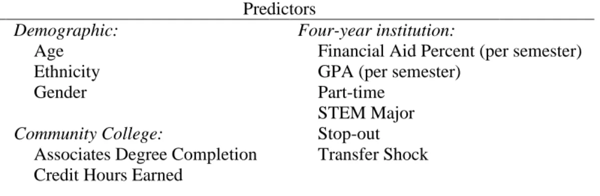
Predictors ... 37
Model-Fitting ... 40
CHAPTER 3: RESULTS ... 42
Descriptive Statistics ... 42
Baseline Hazards ... 46
Model-Fitting ... 48
Full Model ... 50
Event of Interest: Graduation ... 52
Competing Risk: Departure ... 53
Cumulative Hazard Curves ... 54
CHAPTER 4: DISCUSSION ... 65
Substantive Findings ... 65
Implications ... 68
Limitations ... 71
Future Research ... 72
APPENDIX 1: ESTIMATES FOR SCHOOLS ... 76
ix
LIST OF TABLES
Table 1. Example of a Person-Period Dataset ... 27
Table 2. Time Indicators for Example of Person-Period Dataset ... 28
Table 3. Computing Cumulative Hazards for Competing Risk Models ... 31
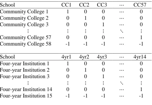
Table 4. Unweighted Effects Coding for Community Colleges and Four-Year Institutions... 35
Table 5. Model Predictors ... 36
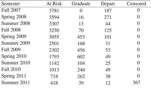
Table 6. Status of NCCCS Transfer Students at the Beginning of Each Semester ... 42
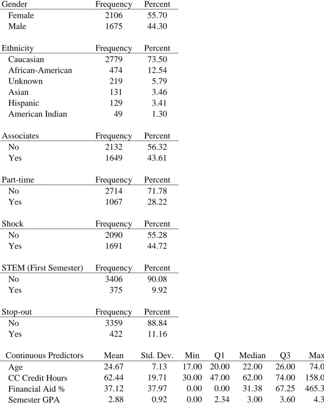
Table 7. Descriptive Statistics for Model Predictors ... 44
Table 8. Frequencies of Community Colleges ... 45
Table 9. Frequencies of Four-Year Institutions ... 46
Table 10. Hazard and Cumulative Hazard Rates for Baseline Model ... 46
Table 11. Model-Fitting Results ... 49
x
LIST OF FIGURES
Figure 1. Example of Right-Censoring ... 19
Figure 2. Simulated Graphs of Hazard and Cumulative Hazard Functions ... 23
Figure 3. Example of Cross-Classification ... 33
Figure 4. Baseline Hazard Functions for Graduation and Depart ... 47
Figure 5. Baseline Cumulative Hazard Curves for Graduation and Depart ... 48
Figure 6. Cumulative Hazard Curves for the Reference Students ... 55
Figure 7. Cumulative Hazard Curves for Caucasian and African-American Males and Females 56 Figure 8. Cumulative Hazard Curves for Age ... 57
Figure 9. Cumulative Hazard Curves for Community College Credit Hours Earned ... 58
Figure 10. Cumulative Hazard Curves for Associate's Degree ... 59
Figure 11. Cumulative Hazard Curves for Financial Aid Percent ... 60
Figure 12. Cumulative Hazard Curves for Semester GPA ... 61
Figure 13. Cumulative Hazard Curves for Part-time and Stop-out ... 62
Figure 14. Cumulative Hazard Curves for Transfer Shock ... 63
1
CHAPTER 1: INTRODUCTION
The study of college completion and student retention has long been an important part of
higher education research, and there has never been a time in history when college completion
has been more emphasized. Policymakers and administrators are setting ambitious goals to
ensure student completion at both two-year and four-year institutions. President Barack Obama
set an ambitious goal for America to have the highest percentage of college graduates in the
world by 2020, including an additional 5 million community college graduates by 2020 (The
White House, 2014).
The Association of American Community Colleges (2014) reports that approximately
11.5 million students are enrolled in two-year community colleges representing 46% of all
undergraduate students in the United States. Nearly half of students who complete a bachelor’s
degree started at a community college (Association of American Community Colleges, 2014, p.
4). During the last several decades, community colleges have experienced tremendous growth in
enrollment. Tuition increases and increased enrollment competition at many four-year
institutions have led to the popularity of the open admissions policy and low tuition offered by
community colleges. One of the major functions of a community college is to provide students
with a means for transferring to a four-year institution for the completion of a bachelor’s degree;
however, only 61.6% of the nation’s community college transfer students complete a bachelor or
higher at a four-year institution within six years after transfer (Shapiro, Dundar, Ziskin, Chiang,
2
Methodological Concerns
In many instances college completion is examined in a cross-sectional manner; that is,
completion rates are obtained by comparing the entering time of a cohort to a future time point
(e.g., 4 or 6 years). A student’s timing of completion and retention is lost; namely, the length of
time it takes a student to complete a degree or the semester in which a student departs college.
However, even with longitudinal data, incorporating time into traditional analyses is difficult
given that students who do not graduate in the time period under consideration are censored; that
is, there is no information on whether or not they will graduate in the future. Additionally, the
use of time-varying predictors, variables that differ during each time period (i.e., GPA), are
difficult to study with traditional statistical approaches.
Survival analysis addresses many of these issues when analyzing student completion
data. In addition to allowing for censored data and time-varying predictors, Willett and Singer
(1991) summarize two additional reasons why survival analysis is superior to traditional methods
for the study of event occurrence such as college completion. First, the time frame being studied
is typically not substantively motivated. If a 4-year completion rate is examined, then any
information about the timing of graduation within the four years is lost. Second, variations in the
length of time periods studied can lead to contradictory results. If one computes 4-year versus
6-year completion rates, it is possible that conclusions on important variables affecting completion
will be different.
While survival analysis has been used in student completion research, it is rarely used to
study transfer student outcomes. To date, there have been only two published applications of
survival analysis using transfer student data (Mourad & Hong, 2008; Hayword, 2011). In both
3
(2008) used a competing risks survival analysis, where the alternative outcome of interest was
transfer to another two-year school. No known study has used survival analysis to examine
bachelor’s degree completion of transfer students.
Study Purpose
This study will utilize discrete-time survival analysis to examine the factors that are
important in predicting if and when a North Carolina community college student will complete
his or her bachelor’s degree at a North Carolina public university. There are three primary goals:
(1) to apply an advanced methodological procedure to analyze transfer student data and provide
researchers with a tutorial of the methodology; (2) to consider the timing of transfer student
completion of the bachelor’s degree; and (3) to study the factors that influence bachelor’s degree
completion of community college transfer students in North Carolina.
The study will examine three research questions of interest about North Carolina
community college students who transfer to a North Carolina public four-year institution:
1. What are the more important factors that influence bachelor’s degree completion and
timing of completion of North Carolina community college transfers?
2. Does earning an associate’s degree influence completion and timing of completion at the
four-year institution?
3. Does “transfer shock” affect the completion and timing of completion of the bachelor’s
degree?
Tinto’s Student Integration Model
Many theories describing student departure from college settings have been formulated,
but Tinto’s (1975; 1993; 2006) student integration model focuses on the interaction of student
4
completion, persistence, and retention (Melguizo, 2001). Understanding student departure is
important for understanding students who persist at an institution and eventually graduate from
that institution. Tinto argues that, because student departure is a process unfolding over time,
longitudinal data should be used to understand why students depart (attrition) as a function of the
institution and the student’s interaction with the institution.
Tinto’s student integration model features two key methods of integration: academic and
social. Academic integration refers to a student’s interaction with faculty both inside and outside
of the classroom. Social integration, on the other hand, refers to students’ social interactions
either in a formal institutional context (such as planned activities) or social interaction with other
students in an informal context. Tinto argues that students who feel academically and socially
integrated in the institution are less likely to depart from that institution. Tinto’s student
integration model has been applied for transfer students and existing research in this area will be
reviewed in a subsequent section.
Expanding Tinto’s model, Bean and Eaton (2000) developed a model that outlines
psychological principles that are thought to be important for a student to integrate academically
and socially into an institution (Tinto, 1975; 1993; 2006). Bean and Eaton (2000) suggest that
students enter the institution with certain psychological characteristics based on previous
experiences, abilities, and self-efficacy assessments. The student then interacts with the
institution academically and socially. During these interactions the student engages in continual
self-assessments connecting her experiences with the institution to her feelings about that
institution. Students use adaptive strategies to integrate academically and socially into the
institution. These strategies are based on three psychological principles: (1) self-efficacy theory;
5
Bean and Eaton (2000) explained that students have self-efficacy when they believe that
they are capable of performing well at the institution, and that based on past experiences and
observation, they will have increased social and academic integration and more persistence. That
is, students who believe they are capable of doing well in a particular major or at a particular
institution will have higher self-confidence and more persistence. Students also develop coping
strategies to adapt to the new environment at the institution. These strategies allow students to
cope with fitting in or not fitting in to the new institution. Finally, students with an internal locus
of control tend to have a better academic and social integration than students with an external
locus of control. With an internal locus of control students believe that their achievements –
academic and social – arise because they consistently work hard and study; whereas, students
with an external locus of control view academic and social success as being due to factors that
are not determined from within. They attribute their success to external factors such as having
good instructors or pure luck. These psychological principles are important for understanding
how a student academically and socially integrates into the institution.
Community Colleges
Community colleges provide access to higher education and eventual completion of the
bachelor’s degree for many students. Most research on community college transfer students has
focused on successful transfer of students from the community college to a four-year institution
and fewer studies have examined successful completion of the bachelor’s degree. However,
several studies have examined factors that predict successful completion of the bachelor’s degree
for community college students at four-year institutions (e.g., Arbona & Nora, 2007; Bailey &
6
Bunn, 1998; Koker & Hendel, 2003; Mourad & Hong, 2011; Roksa & Keith, 2008; Wang,
2009).
Previous research on student completion has been mixed with respect to which specific
demographics are the strongest predictors of completion. Studies have found female transfer
students are less likely to graduate after transferring (Freeman, 2006; Surette, 2001), more likely
to graduate (Wang, 2009), or that there is no effect for gender (Koker & Handel, 2003). It has
also been shown that older students are less likely to graduate (Freeman, 2006; Henry & Knight,
2003), while another study suggests there is no effect of age (Koker & Handel, 2003).
Additionally, underrepresented minority students are less likelyto complete than Caucasian
students (Anglin, Davis & Mooradian, 1995; Pincus & Archer, 1989); however, at least one
study found no effect for ethnicity (Wang, 2009). Finally, lower income students are less likely
to complete (Wang, 2009).
Higher completion rates are reported among community college transfer student who
complete an associate's degree (Cejda & Rewey, 1998), transfer with more community college
credit hours (House, 1989), and have a higher community college GPA (Koker & Hendel, 2003;
Townsend, McNemy & Arnold, 1993). Among the predictors of degree completion in four-year
institutions, factors such as full-time enrollment (Roksa, 2006) and continuous enrollment
(DesJardins, Ahlburg, & McCall, 2006) are both important factors in the likelihood that a student
will complete (Roksa, 2006). Furthermore, STEM majors starting at community college are less
likely to graduate from four-year institutions (Wang, 2013). It is important to understand what
7
Community College Mission
The overall mission of the community college is to “provide access to postsecondary
educational programs and services that lead to stronger, more vital communities” (Vaughan,
2006, p. 3). The core value of the community college is to provide access to higher education for
all members of the community. To ensure this equality, community colleges adopt an open
admissions policy where any member of the community has the opportunity to enroll in college.
However, an open admissions policy is not the only way community colleges provide access and
equality. Vaughan (2006) explains that community colleges must be located within a reasonable
distance from students within the area they serve, provide appropriate student support while
students are enrolled, and ensure equal access to all members of the community regardless of
gender, race or socioeconomic status.
Another important aspect of an open enrollment policy includes providing comprehensive
program offerings (Vaughan, 2006). Community college program offerings can be grouped into
five types including: (1) vocational education, (2) developmental education, (3) continuing
education, (4) community education, and (5) academic transfer (Cohen & Brawer, 2008). In
general, vocational, developmental, continuing, and community education set community
colleges apart from typical four-year institutions. Vocational (sometimes referred to as technical
or occupational) programs are terminal programs in career-based fields that community colleges
offer at both the associate and baccalaureate levels. Developmental education courses offered by
community colleges allow students who are not ready for college level work to obtain the
necessary skills they need in reading, writing, and math. Continuing and community education
refers to courses and programs that allow members of the community to further their education
8
offerings at community colleges, academic transfer, refers primarily to transfer programs
designed to provide students with general education requirements and a gateway to a four-year
college.
The Transfer Function
Academic transfer, also called the transfer function, is one of the most important
functions of the community college. The transfer function exists to accept students from high
school and provide them with general education courses at the collegiate level to prepare them
for the baccalaureate at a four-year institution. Because many students at community colleges are
minority and low-income students, the transfer function is an important way for a community
college to reach the entire community in which it serves (Cohen & Brawer, 2008).
The literature on transfer student data lacks consistency on the definition of a community
college transfer student. The classification of a transfer student also varies across four-year
institutions. There are two primary factors to consider when determining if someone is a
community college transfer student. First, while it appears evident, to be considered a
community college transfer student, the student must have transferred from a community college.
Second, students must have taken a specified minimum number of credit hours at a community
college to be considered a transfer student. The literature is not clear on what this minimum
should be, but many four-year institutions in North Carolina consider a student to be a transfer
student if he or she has taken at least 24 or 30 credit hours (or approximately 8-10 courses) at
another institution. For the purposes of this study, a North Carolina community college transfer
student is defined as a student who: (1) transfers from a North Carolina community college; and
9
Transfer Shock
Transfer shock is a term that refers to a decline in GPA of community college students
during their first semester at a four-year institution (Hills, 1965). There are many reasons why
transfer shock might occur, but several studies have noted differences in the likelihood of
transfer shock based on demographic factors (Dennis, Calvillo, & Gonzalez, 2008; Durio,
Helmick, & Slover, 1982), preparation of the student (Dennis et al., 2008; Reason, 2003),
academic major (Cejda, 1997; Cejda et al., 1998), and adjustment to a new educational
environment (Berger & Malaney, 2003). Hills (1965). Some researchers (Nolan & Hall, 1978;
Diaz, 1992) explain that many students show evidence of recovery from transfer shock; however,
when recovery is not achieved, transfer shock may delay degree completion or be a source of
attrition for transfer students.
Diaz (1992) conducted a meta-analysis of transfer shock and found that out of a total of
62 studies that measured a decline in GPA during the first semester or quarter of transfer,
forty-nine determined students had experienced transfer shock with most reporting a GPA change of
0.5 points or less. Recovery from transfer shock, i.e., returning to GPA at or similar to the
community college GPA, was found in 67% of the 49 studies reporting evidence of transfer
shock and recovery occurred typically within the first year after transfer. Transfer shock is well
documented in the literature, and many four-year institutions specifically advise transfer students
about this phenomenon after transferring from community college to a four-year institution.
Glass and Harrington (2002) suggest the use of counseling, tutoring and mentoring as methods of
helping students overcome transfer shock and integrate academically and socially into the
10
Academic and Social Integration of Transfer Students
Tinto’s student integration model (1975; 1993; 2006) has been used as a primary
theoretical framework for understanding the perspective of traditional, native four-year students.
Fewer studies have applied the model to transfer students at four-year institutions; however,
some studies have shown usefulness in Tinto’s model for community college students (Halpin,
1990). Pascarella and Chapman (1983) report that academic integration played a stronger role in
persistence for students at two-year institutions than social integration. Furthermore, Bean and
Metzner (1985) developed a student integration model specifically for nontraditional students at
four-year commuter institutions. The model puts more emphasis on external variables, i.e.,
employment, family responsibilities, etc. The authors suggest that external variables are more
important than academic and social integration for predicting departure of a nontraditional
student. That is, nontraditional students who receive high external support and have high
satisfaction are less likely to depart.
While there is some work on academic and social integration experiences for transfer
students, the impact of academic and social integration on persistence in higher education has
been well documented. Several studies have used surveys and interviews to examine the
academic environment of transfer students at four-year institutions (e.g., Flaga, 2006; Glass &
Bunn, 1998; Townsend, 1995; Townsend, 2008; Townsend & Wilson, 2006). Measures used in
these studies typically focus on classroom interactions and perceptions of the academic
environment. The studies show there are differences in academic integration at four-year
institutions and community colleges, and it is highlighted by the interaction between students and
faculty at each of these institutions. Townsend (2008) stated that some community college
11
daunting (p. 73),” and Townsend (1995) reported that transfer students felt that community
college faculty were more helpful than faculty at four-year institutions. Transfer students have to
adapt to the new academic environment and a different relationship with faculty at the four-year
institution. It is this disconnect that can initially be a source of transfer shock for community
college transfer students at the four-year institution.
Several studies have examined social integration of community college students into the
four-year institution (e.g., Bahr et al, 2013; Laanan, 2007; Owens, 2010; Reyes, 2011; Townsend
& Wilson, 2006). These studies have used surveys and interviews to measure social integration
and primarily focus on social adjustment of the transfer student. Townsend and Wilson (2006)
reported that some transfer students had trouble making friends and difficulty adjusting socially
to the new environment; however, it has been shown that transfer students involved in clubs and
organizations have less negative social adjustment (Laanan, 2007). Transfer students are in the
unique position of having to adapt to new social environments that already exist among native
students. Additionally, transfer students often have other responsibilities, such as employment
and family, which utilizes a majority of their free time and leads to poor social integration into
the four-year institution (Bahr et al, 2013; Owens, 2010; Reyes, 2011).
North Carolina Higher Education System
To better understand the academic environment of North Carolina community college
transfer students, I will describe the North Carolina Higher Education System, which includes
the community college system and public four-year institution system. The North Carolina
Community College System (NCCCS) consists of 58 public community colleges making it the
third largest community college system in the nation (NCCCS, 2014). An estimated 840,000
12
citizens who are age 18 years or older (NCCCS, 2014). The mission of the NCCCS is “to open
the door to high-quality, accessible educational opportunities that minimize barriers to
post-secondary education, maximize student success, develop a globally and multiculturally
competent workforce, and improve the lives and well-being of individuals by providing: (1)
education, training and retraining for the workforce, including basic skills and literacy education,
occupational and pre-baccalaureate programs; (2) support for economic development through
services to and in partnership with business and industry and in collaboration with the University
of North Carolina System and private colleges and universities; and (3) services to communities
and individuals, which improve the quality of life” (NCCCS, 2008, p. 3). The University of
North Carolina (UNC) System comprises 16 institutions of higher education, as well as a
residential high school for gifted students called the North Carolina School of Science and Math.
An estimated 220,000 students are enrolled in the UNC System with a mission to “discover,
create, transmit, and apply knowledge to address the needs of individuals and society”
(University of North Carolina, 2014).
Recent Legislation
In recent years the North Carolina Community College System has been developing
performance-based measures to be included in the budget allocation formula for the state’s
community colleges. Eight performance-based measures were adopted in June 2012, and the
inaugural report utilizing these measures was released in June 2013. One of the new measures is
intended to assess student success after transferring to a four-year institution from a North
Carolina community college. It is measured by calculating the percentage of transfer students
13
defines a transfer student to have completed an associate’s degree or accumulated at least 30
articulated transfer credits.
While the college transfer performance measures do not directly measure bachelor’s
degree completion at the four-year institution, it is a measure of successful completion of the
transfer student within the first year. The remaining measures all focus on completion,
progression or passing rates, which highlights the emphasis being placed on completion both
directly and indirectly. In the past, enrollment was the metric used for budget decisions; but the
importance of degree completion and progression is becoming more prominent within the North
Carolina Community College System.
Articulation Agreement
The NCCCS and UNC System have created an articulation agreement between all 58
community colleges in North Carolina and all sixteen four-year universities. The Comprehensive
Articulation Agreement (CAA) governs the transfer of credits between community college and
four-year institutions in North Carolina. It also outlines the Transfer Assured Admissions Policy
(TAAP). The TAAP assures community college students admission into one of the sixteen UNC
System institutions if the student: (1) earns an associate’s degree; (2) has an overall GPA or 2.0
or better; and (3) earned a C or better in all CAA general education courses. The articulation
agreement is important because it creates a partnership between the NCCCS and UNC System.
Even if the student does not participate in the TAAP, the CAA allows for a more seamless
transition for students when transferring into a four-year institution in North Carolina. The CAA
outlines transferable courses so students know exactly what will transfer and what will not
14
Articulation agreements such as these are extremely important to the transfer function of
the community college and a transfer student’s integration into the four-year institution. It creates
an environment where students can transition into the four-year institution without having to
worry about credits not transferring correctly. Ideally, it creates a seamless connection from
community college to a four-year institution. This type of agreement makes the study of North
Carolina Community College transfer students within the UNC System more important because
the NCCCS and UNC System are providing community college students the opportunity to
continue their education at the bachelor’s level. The focus of the current study will be to use
survival analysis techniques to identify the factors (e.g., transfer shock, associate’s degree
completion, four-year institution GPA) that are important in this transition and completion of the
15
CHAPTER 2: METHODOLOGY Survival Analysis
Survival analysis is a set of statistical methods that allow researchers to model time-to-event data. Time-to-event data are longitudinal data that measure time from a starting point until the occurrence of an event of interest. Timing of events is a common research question in the
social and behavioral sciences (e.g., completion of college, duration of marriage, time to
puberty), and these questions typically seek to determine “whether events occur” or “when
events occur” (Singer & Willett, 2003, p. 306). That is, survival analysis studies both the
occurrence and timing of an event.
One common technique of modeling data with a dichotomous outcome is logistic
regression. However, traditional logistic regression is limited in two ways: (1) it only considers if
the event occurs; it does not model the timing to event occurrence and (2) traditional logistic
regression models are not able to handle censored data, i.e., data where the measurement of the
outcome is partially known.
Survival analysis originated in the epidemiology and biostatistics literature (Cox, 1972),
but became more popular in the social sciences over the last two decades (Singer & Willett,
1991). The name survival analysis originates from the event of interest being death in the early
development of survival analysis (Allison, 2010b). In this context it was used to study the time to
death after being diagnosed with a disease, given treatment or following surgery. While
somewhat morbid, it is important to understand the beginning of survival analysis to understand
16
Depending on the research question and academic field, there are various terms used to
describe survival models, such as event history analysis, duration analysis, reliability analysis
and transition analysis (Box-Steffensmeier & Jones, 2004). All of these models are concerned
with time-to-event analysis. Furthermore, the term “survival” is a misnomer in many applications; that is, “surviving” a certain event is not of concern but rather the concern is
studying time to event occurrence. For example, in context of college completion, “surviving”
refers a student who did not complete college, i.e., did not experience the event.
Another key term in survival analysis is “risk.” Survival models assume that everyone is
“at risk” of the event occurring. Once again, the terminology is rooted in the early days of
survival analysis where individuals contracted a disease and they were considered “at risk” of
death. For college completion, students are “at risk” of graduating from college given they did
not graduate in a previous semester. That is, every student that enrolls in college is “at risk” of
graduating but when a student graduates, he or she is no longer at risk.
Discrete versus Continuous Time
The measurement and assumption of time is critical in developing the proper survival
analysis model. Time scales for survival analysis can be categorized into continuous or discrete
time. Distinguishing between the two time scales is important in choosing whether a
time or continuous-time survival model should be used. In the social sciences typically
discrete-time models are preferred over continuous-discrete-time models for several reasons (Allison, 2010a;
Singer & Willett, 1993). First, discrete-time models allow for the easy inclusion of time-varying
predictors; whereas, many continuous models require more sophisticated software to incorporate
17
survival analysis are easier to understand. Finally, time is often measured discretely and these
data would not be appropriate for a continuous model (Singer & Willett, 1993).
Continuous-time events occur when the exact time of the event is known (e.g., time of
death) and discrete-time events occur when events occur at discrete points in time (e.g.,
graduation from college). Allison (1982) describes two situations for assuming discrete-time
events: (1) whenever events actually occur at discrete points in time; and (2) whenever the data
record events at discrete points in time. For example, students complete courses only one time
per semester so those data are only available in discrete points in time (i.e., at the end of each
semester). In the second situation a student might dropout at any point in time during the
semester, but typically that information is only available at the end of each semester; thus, the
event is recorded in discrete points in time even though it is really more of a continuous process.
Clearly, for the first situation described above, a discrete-time model is appropriate given
time is measured on a discrete scale. However, in the second situation there are two possible
approaches: (1) treat time as continuous and use a continuous survival model correcting for the
discrete nature of the data; or (2) treat time as discrete and use a discrete survival model. Given
the advantages of the discrete-time model and that model specification is not affected by either
of the approaches described above (Allison, 1982), a discrete-time model is preferred.
Furthermore, Vermunt (1997) explains that discrete-time methods can be used to approximate
continuous-time methods. Given the complexities of the continuous-time survival models and the
more frequent need for discrete-time models in the social sciences, a discrete-time survival
18
Censoring
One of the main advantages of the survival model is the ability to handle censored data.
These data occur because individuals in the dataset will either never experience the event or did
not experience the event during the time frame being studied (Singer & Willett, 2003). That is,
censoring occurs when the event does not occur during the time frame being studied or a
participant leaves prior to the end of the study. Censoring is another term for missing data. When
data are censored, there is incomplete knowledge of when or if the event occurred; therefore,
those data are considered missing.
Censoring can be categorized into right-censoring and left-censoring. Left-censoring
occurs when the event of interest is experienced before the time frame being studied; whereas right-censoring occurs when the event of interest is experienced after the time frame being studied. For instance, a student may not complete college in a particular time frame being
observed; this is an example of right-censoring. Left-censoring is impossible in the present study
because students are being tracked beginning at a particular semester, i.e., none could have
graduated college prior to the first semester.
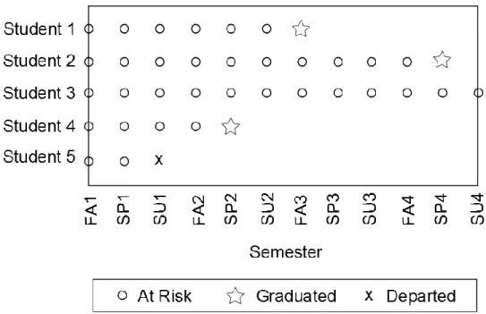
Figure 1 shows a simple example of five transfer students who were followed for four
years (or 12 semesters). The open dots represent the semesters the students are “at risk” of either
graduating or departing from the institution. If a student graduates in a given semester, that is
represented by a star and if a student departs, that is represented by an “x.” In the graph students
1, 2, and 4 all graduated. Student 4 completed in two years, and Students 1 and 2 took longer
than two years. Additionally, Student 5 departed the college in the summer of his or her first year
and Student 3 had not graduated by the end of the time period. For the purposes of this study,
19
Figure 1. Example of Right-Censoring
There are two important classifications of censoring: informative and non-informative.
Non-informative censoring is censoring that is due to random occurrence and is much like
missing-at-random (MAR) in the missing data literature (Rubin, 1976). For instance, the
censoring from students not completing college by spring of the fifth year is non-informative
censoring1. That is, the students are not taking actions to cause the censoring; instead, the
censoring occurs because the data collection ends at that point in time. Student 3 is an example
of non-informative censoring in Figure 1. Conversely, informative censoring is censoring that is
not random and due to a systematic reason (i.e., dropout or transfer). For example, Student 5
departed during the summer of his or her first year, which is unlikely a random occurrence and
the departure is most likely due to dropout or transfer. Survival models require that censoring be
1 It can be argued that the longer the student is at risk of completing, the less likely that student is to complete. This
20
non-informative. In this context, departure is considered to be a competing risk for graduation,
which will be discussed in a subsequent section.
The Survival Model
The foundation of survival analysis lies in three important functions: the density function,
the survivor function and the hazard function. In this section all three functions will be defined,
and the relationship between the functions will be discussed. To begin, let Ti be a discrete
random variable indicating the event time (i.e., semester of graduation) for student i where i = 1, 2, …, N.Let j indicate each semester where j = 1, 2, …., J. The density function is written as
𝑓𝑖(𝑗) = P(𝑇𝑖 = 𝑗). (1)
This function defines the probability of graduation occurring during semester j for student i. However, there are problems with defining the density function in this manner when using
censored data. For example, if a student graduates in his or her second year, then the probability
that he or she graduates in the third year is meaningless. Therefore, there needs to be a better way
to determine the probability.
Another formulation of determining probability of graduation occurring during semester j
is to find the probability of “surviving” graduation. From this point forward, the subscript i will be omitted indicating that the random variable is for a random student in the population;
however, it is important to realize that each student can have his or her own trajectory. The
survivor function, 𝑆(𝑗), is the probability that graduation has not occurred in semester j and is written as
𝑆(𝑗) = P(𝑇 > 𝑗) = 1 − 𝐹(𝑗) (2)
where 𝐹(𝑗) = ∑𝑗𝑘=1𝑓(𝑗) is the cumulative distribution function. The survivor function
21
mentioned before, the term “survive” is a misnomer in the current application, i.e., students who
“survive” college are students who do not graduate. Thus, this survivor function represents the
probability that a randomly selected student does not graduate. Notice that the survivor function
is written as a function of the cumulative density function. However, this approach makes the
assumption that all students will eventually experience graduation (i.e., 𝑓(𝑗) is known), which
may or may not be true in the presence of censored data.
Given the problems using the density function and using the survivor function with
censored data, it is important to develop a function that can be estimated even with the presence
of censoring. The hazard function, ℎ(𝑗), is the conditional probability that graduation will occur
in semester j, given that it did not occur at an earlier semester for that student. This function is written as
ℎ(𝑗) = P(T = j|T ≥ j). (3)
The hazard function is conditional in nature, meaning that only students who are eligible to
graduate are included. These students represent the so-called “risk set.” The risk set is a set of
students who are “at risk” of graduating, i.e., students who have not graduated in a prior semester
are at risk of graduation.
Finally, there is an important relationship between the survivor function and the hazard
functions. More specifically, the survivor function can be written in terms of the hazard functions
by
𝑆(𝑗) = ∏[1 − ℎ(𝑘)]
𝑗
𝑘=1
. (4)
This equation shows that the survivor function probability at semester 𝑗 is simply the product of
22
survivor function and the hazard function allows for the estimation of the survivor function even
with censored data.
As mentioned, in the context of student completion, survivor functions represent the
proportion of students who have survived graduation for a given semester 𝑗. Therefore, if the
proportion who survived graduation is subtracted from one, that value represents the proportion
of students who actually graduated for a given semester 𝑗. In this context it makes more sense to
present curves that report the proportion of students who graduated. To do this, the cumulative
hazard, 𝑀(𝑗), is defined as
𝑀(𝑗) = 1 − 𝑆(𝑗) = 1 − ∏[1 − ℎ(𝑘)].
𝑗
𝑘=1
(5)
From this point forward, the cumulative hazard function will be used instead of the survivor
function.
Graphing the Hazards and Cumulative Hazards
One of the unique features of survival analysis is the ability to examine graphs of hazards
and cumulative hazards. Hazards are estimated across different values of time and can be plotted
against time. This plot provides a profile for the unique risk of an event at each time point (i.e.,
event did not occur at another time point). Furthermore, the cumulative hazards can be plotted
against time using the relationship defined in Equation 5. This plot shows the probability that a
randomly selected person has experienced the event.
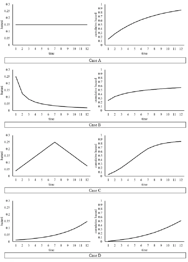
Figure 2 shows an example of four different hazard functions and their corresponding
cumulative hazard functions. Hazard functions are characterized by peaks and troughs. During
23
24
likely to graduate); conversely, during the troughs the magnitude is low, indicating a lower risk
(i.e., students are less likely to graduate). Examining the hazard probability graph gives a general
picture of the profile of risk over time. The four scenarios depicted in Figure 2 show four
different patterns of hazard probabilities over time. Case A features hazard probabilities that are
constant over time. While this type of risk profile is rare in the social sciences, it does illustrate
the possibility of having hazard probabilities that are independent of time. For the scenario in
Case B, the hazard is highest at the first time point then decays across time. This hazard is a
common pattern in the social sciences especially in recurrence and relapse data because the risk
of recurrence tends to be greatest following treatment. Another possibility is where hazard peaks
at a particular point intime as depicted in Case C. The hazard probabilities are low at first,
increase to a particular point and then decrease. A similar type of scenario would be common in
student completion data as the risk of graduating increases to a particular point. Finally, the last
type of scenario depicted in Case D shows the hazard probabilities monotonically increasing
across time.
In Figure 2 many of these properties for the cumulative hazard curves can be seen. Cases
B, C, and D show that when the hazard probability is high, then the cumulative hazard
probability increases rapidly. Likewise, when the hazard probability is low, the cumulative
probability increases at a slower rate. When hazard remains unchanged across time as in Case A,
the cumulative hazards increase at a steady rate across time. Cumulative hazard plots are very
useful in displaying findings from a study because they take into account the hazard at each time
period and cumulate these risks over time. They provide readers with a quick and relatively easy
25
In the context of student completion students are followed over time to examine
graduation rates, the cumulative hazard function will be at zero across the first few semesters
because no one is graduating. After the first few semesters, there will be an increase in the
cumulative hazard function because many of the students will be graduating. The cumulative
hazard probability at the last time period represents the proportion of students who have
graduated at that point in time. Finally, the median time-to-degree can be determined for the
cumulative hazard plot; that is, the time point where 50% of the students have graduated.
The Hazard Function
As discussed, the hazard function is most useful in the presence of censored data and the
hazard probabilities are typically used as the dependent variable of the survival model (Singer &
Willett, 2003). However, the hazard function is a probability bounded between 0 and 1, which
creates a problem when fitting discrete-time survival models because predicted values may lie
outside of the boundary. To overcome this problem, the hazard function can be transformed to an
unbounded scale via a link function, which can be the inverse of any cumulative distribution
function. However, the most popular link function is the logit (Singer & Willett, 2003) first
proposed by Cox (1972). The primary advantage to using the logit transformation is the
familiarity of the function with researchers and its availability in software packages. Given these
reasons, the logit link function is used from this point forward. Applying the logit to the hazard
function in Equation 3, the following is obtained
𝑙𝑜𝑔𝑖𝑡 ℎ(𝑗) = 𝑙𝑛 ℎ(𝑗)
1 − ℎ(𝑗) = 𝛼(𝑗) (6)
26
Adding Predictors
While the baseline model can be of interest, the ultimate goal is to include predictors to
the model. Both time-invariant and time-varying predictors can be included in the hazard.
Suppose there are a set of 𝑃 time-invariant and 𝑄 time-varying predictors, let 𝑿be a 𝑃 𝑥 1 vector
of time-invariant predictors and 𝒁𝒋 a 𝑄 𝑥 1 vector of time-varying predictors at semester 𝑗. The
model in Equation 6 can be rewritten to include the predictors
𝑙𝑜𝑔𝑖𝑡 ℎ(𝑗) = 𝛼(𝑗) + 𝛽𝑗′𝑋 + 𝜅𝑗′𝑍𝑗 (7)
where 𝜷𝒋′ represents the vector of slope parameters for time-invariant predictors and 𝜿𝒋′ is the
vector of slope parameters for the time-varying predictors for semester 𝑗. Just like in a linear
regression model, each slope parameter represents the change in the baseline logit hazard
function given a one-unit increase in the predictor, holding all other predictors constant. It is
important to note that Equation 7 allows for the effects of time-invariant predictors to vary across
semesters; however, the proportional odds assumption can be invoked by constraining the effects
to be the same across semesters, i.e., 𝜷′. Furthermore, the intercept parameter 𝛼(𝑗) represents
logit hazard value for semester j when all the predictors are zero. As in linear regression, the hazard model can handle both categorical and continuous predictors.
Estimating the Model
The model can be estimated using a logistic regression procedure in many standard
statistical programs when the data are in the person-period format. A person-period data are
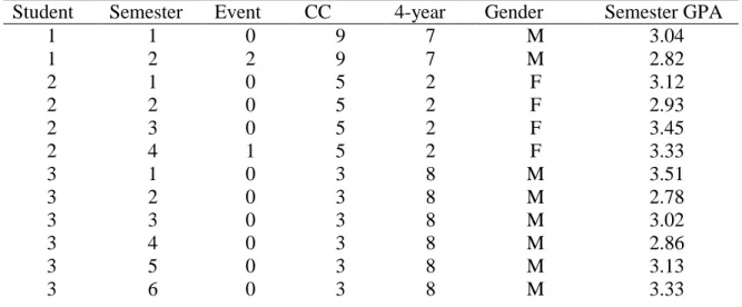
those that contain multiple rows for each student. Table 1 shows a hypothetical example of a
person-period dataset for three students over six semesters. The EVENT variable indicates the
semester in which a student graduates or departs the university. Graduation occurred if EVENT
27
the student did not graduate or depart, EVENT = 0. For the example in Table 1, Student 1
departs the institution during the second semester, Student 2 graduates in her fourth semester and
Student 3 is censored, i.e., does not graduate or depart during the six semesters being studied.
The inclusion of time-invariant and time-varying predictors are entered into the
person-period dataset as additional columns. A time-invariant predictor remains the same across rows
for each student but a time-varying predictor changes for each semester. For the example in
Table 1, GENDER, CC and 4-YEAR are time-invariant so they remain the same across
semesters for each student. The indicators CC and 4-YEAR identify the community college and
four-year institution each student attended. Finally, semester GPA is time-varying so it changes
each semester for each student.
Table 1. Example of a Person-Period Dataset
Student Semester Event CC 4-year Gender Semester GPA
1 1 0 9 7 M 3.04
1 2 2 9 7 M 2.82
2 1 0 5 2 F 3.12
2 2 0 5 2 F 2.93
2 3 0 5 2 F 3.45
2 4 1 5 2 F 3.33
3 1 0 3 8 M 3.51
3 2 0 3 8 M 2.78
3 3 0 3 8 M 3.02
3 4 0 3 8 M 2.86
3 5 0 3 8 M 3.13
3 6 0 3 8 M 3.33
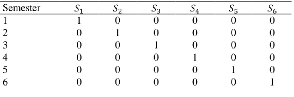
For the example in Table 1, time is indexed by SEMESTER. One possible representation
of time is to create dummy variables for each semester as time indicators using 𝐽 indicators for
𝐽 semesters. Table 2 gives the time indicators for the person-period dataset presented in Table 1.
28
each 𝛼(𝑗) is the logit hazard probability estimate or intercept for semester j. This representation is preferred because it is easiest to interpret.
Table 2. Time Indicators for Example of Person-Period Dataset
Semester 𝑆1 𝑆2 𝑆3 𝑆4 𝑆5 𝑆6
1 1 0 0 0 0 0
2 0 1 0 0 0 0
3 0 0 1 0 0 0
4 0 0 0 1 0 0
5 0 0 0 0 1 0
6 0 0 0 0 0 1
Interpreting the Parameters
Parameter interpretations are similar to multiple regression, except now the dependent
variable is a logit. First, consider the situation where the predictor is binary and dummy coded
with two categories, category 0 (reference) and category 1. The intercept 𝛽0 is the value log odds
of the DV for the reference category and the slope 𝛽1 represents the change in log odds in the
DV from the reference category to category 1. For ease of interpretation, it is helpful to offer an
interpretation in terms of an odds ratio. To do this, Equation 6 can be expressed in terms of odds
by taking the exponential of both sides resulting in
ℎ(𝑗)
1 − ℎ(𝑗)= 𝑒
𝛽0+𝛽1𝑋. (8)
The odds ratio, OR, is defined as the ratio of the event occurring in one category and the event
occurring in the other category. Thus,
𝑂𝑅 = 𝑒
𝛽0+ 𝛽1(1)
𝑒𝛽0+ 𝛽1(0) =
𝑒𝛽0+ 𝛽1
𝑒𝛽0 =
𝑒𝛽0𝑒𝛽1
𝑒𝛽0 = 𝑒
𝛽1. (9)
Therefore, the odds ratio for a single binary predictor logistic regression is expressed as 𝑒𝛽1.
For a continuous predictor, the intercept 𝛽0 now represents the value log odds when 𝑋 =
29
written in terms of an odds ratio the same way as with a binary predictor. Consider a one-unit
increase in X, then the OR is
𝑂𝑅 = 𝑒
𝛽0+ 𝛽1(𝑋+1)
𝑒𝛽0+ 𝛽1𝑋 =
𝑒𝛽0+ 𝛽1𝑋+𝛽1(1)
𝑒𝛽0+ 𝛽1𝑋 =
𝑒𝛽0+ 𝛽1𝑋𝑒𝛽1
𝑒𝛽0+ 𝛽1𝑋 = 𝑒
𝛽1. (10)
Thus, for every one-unit increase in X, the odds of Y is multiplied by 𝑒𝛽1. Notice that if 𝛽
1 > 0
(on the log odds scale), then 𝑒𝛽1 = 𝑂𝑅 > 1 (on the odds scale) meaning that the odds increase
for a one unit increase in X. Similarly, if 𝛽1 < 0, then the odds decrease for a one unit increase
in X.
Survival Model for Transfer Student Data
When fitting a discrete-time survival model in the context of transfer student data, there
are a couple of points to consider. First, departure serves as a competing risk to graduation as to
why students leave the institution; thus, a strategy to handle this needs to be considered. Second,
community college transfer students belong to both a community college and a four-year
institution; therefore, the model needs to be specified to allow for this. Modeling techniques for
these issues will be discussed.
Competing Risks
Each semester, students have the possibility of graduating or departing the institution.
Students who depart the institution may either dropout or transfer to another institution.
However, given the constraints on how the data are collected in this study, there is no distinction
made between the two. Likewise, there is no distinction made between students who dropout for
either academic or disciplinary reasons. Stopping out is defined as a student who returns to the
institution after an absence of at least one semester. Students who stop-out and do not return
30
students who have not completed by the end of the time period being studied and have not
departed the institution are censored.
In the present study, graduation from the four-year institution is the outcome of interest;
however, departing the institution is considered a competing risk. That is, not experiencing
graduation and departure are both completing reasons why a student is still “at risk” by the end
of the time period being studied. A distinguishing feature of competing risks is that only one of
these events will occur, or not occur, during a student’s time in college. That is, a student will not
both depart the institution and graduate from that institution.
In survival analysis the competing risk model allows researchers to examine multiple
events of interest. The present study will consider departing the institution as a competing risk of
graduation. To do this, the dataset must contain a variable that identifies the semester a student
departed the university. Allison (1995) describes how separate analyses for each event can be
performed without producing biased parameter estimates and only a slight loss of precision. This
allows the researcher to focus on the event of interest and allows for different models to be
considered for different types of events. Fitting the graduation model, for example, involves
treating students who departed as being censored. However, this treatment invokes an
assumption of non-informative competing risks, i.e., experiencing a particular event tells us
nothing about experiencing the other event.
Non-informative censoring in the competing risk framework assumes that if a student
who experienced a competing event had not done so, the student would be at the same risk of
experiencing the other events as those who did not experience the competing event. That is, if a
student departs then that student would have been at the same risk as the other students for
31
be equally likely to graduate in subsequent semesters as students who eventually graduate. In the
presence of possible informative competing risks, Singer and Willet (2003) suggest including
predictors that are related to both events, i.e., GPA. Including these predictors allows for the
events to be treated as if they are non-informative.
Computing cumulative hazard curves for competing risk models using Equation 5 will
produce incorrect cumulative hazard curves for each event in the competing risks framework.
This will be illustrated by a simple example. Consider the situation given in Table 3 where 100
students are at risk of graduation. During the first semester five students graduated and 15
students departed. Therefore, the hazard for graduation is 0.05 and the hazard for departure is
0.15; that is, 5% of students graduated and 15% of students departed in semester 1. This means
that 80 students are at risk of graduation or departure in semester 2 because a total of 20
graduated or departed during semester 1. Now consider that during the second semester 40
students graduated and 20 students departed; thus, the hazard for graduation is 0.50, and the
hazard for graduation is 0.25.
Table 3. Computing Cumulative Hazards for Competing Risk Models
Hazard Cumulative Hazard
Semester At risk Graduate Depart Graduate Depart Graduate Depart Either
1 100 5 15 0.05 0.15 0.05 0.15 0.20
2 80 40 20 0.50 0.25 0.45 0.35 0.80
The cumulative hazard for each event during the first semester will be the same as the
hazards because there is nothing to cumulate. Notice, there is a column titled “either” in Table 3
showing the cumulative hazard for experiencing either graduation or departure in a given
semester. It is simply the sum of the cumulative hazards of graduate and depart. During the first
semester 20% of the students either graduated or departed. For the second semester, the
32
cumulative hazards can be calculated from taking the total number of students who experienced
the event in the first two semesters and dividing by the number who were initially at risk (i.e.,
100).
Using Equation 5 to calculate the cumulative hazard for the second semester will result in
an incorrect value. For example, computing the cumulative hazard for graduate for semester 2
using Equation 5 yields 1- [(1-.05)(1-.50)] =0.525. This value is greater than the true value
for the cumulative hazard because it is ignoring the other competing risk. Scott and Kenny
(2005) provide an alternative method for computing cumulative hazard when using a completing
risk model to remove this “accounting error.” Let ℎ𝑘(𝑗) be the hazard for event 𝑘, 𝑀𝑘(𝑗) be the
cumulative hazard for event 𝑘 where 𝑘 = graduate or depart, and 𝑀(𝑗) be the cumulative hazard
for experiencing either graduation or departure during semester 𝑗. The cumulative hazards are
defined as
𝑀𝑘(𝑗) = ℎ𝑘(𝑗)[1 − 𝑀(𝑗 − 1)] + 𝑀𝑘(𝑗 − 1) (11)
where 𝑗 > 1, 𝑀𝑘(1) = ℎ𝑘(1) and 𝑀(𝑗) = ∑ 𝑀𝑘 𝑘(𝑗). Calculating the cumulative hazard for
graduation during semester 2 using Equation 11 yields 0.50 [1-0.20] +0.05=0.45, which is the
correct cumulative hazard.
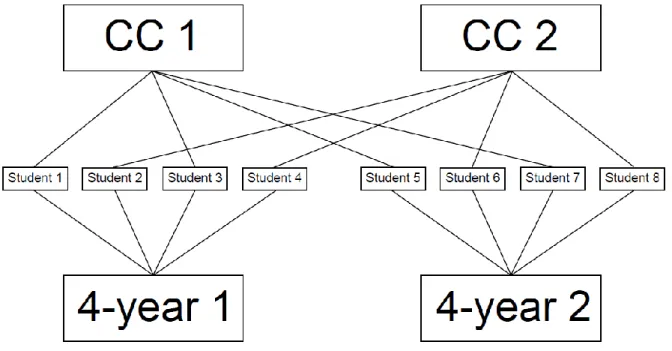
Cross-Classification
A unique feature involved in the analysis of transfer student data is that students belong
to two institutions, i.e., a community college and a four-year institution. This type of scenario in
which an individual is a member of two schools is known as cross-classification in the
multi-level modeling literature. Figure 3 shows an example of the cross-classification in transfer
student data. In this simple example there are two community colleges and two four-year
33
institution 2. Students 1, 3, 5, and 7 transferred from community college 1 and students 2, 4, 6,
and 8 transferred from community college 2. It is important to note how each student belongs to
two institutions. For example, student 1 belongs to community college 1 and 4-year institution 1.
Figure 3. Example of Cross-Classification
The cross-classification means that students are nested within community colleges and
four-year institutions; thus, it is possible that students attending the same community college and
four-year institutions have similarities in graduation or departure. This nesting creates
dependence among observations and violates independence assumptions of the error term, which
can lead to incorrect inferences of parameters. To correct this, typically a random-effects (i.e.,
multilevel modeling) or a fixed-effects approach is used.
The primary difference between a random-effects approach and fixed-effects approach
for nested data is how the schools are added into the model. The fixed-effects approach includes
34
randomly sampled from a population of schools. Both approaches account for school effects;
however, the random-effects approach allows for inferences about a population of schools.
Because all community college and four-year institutions are included in the current study, there
is no sampling of schools. Furthermore, the current study is interested in individual-level effects
and only concerned with controlling for school-level effects. Therefore, a fixed-effects approach
will be utilized.
There are two primary methods for including schools as fixed factors into the model: (1)
dummy coding; and (2) effects coding. Dummy coding specifies a reference school to which all
other schools are compared. Thus, the 𝛼(𝑗) would represent the logit hazard value for semester j
for students belonging to the reference community college and reference four-year institution.
Given the interest is not just one particular school and there is no reason to assign a particular
reference community college or four-year institution, effects coding is more appropriate. Effects
coding specifies a base school but now the 𝛼(𝑗) represents the mean logit hazard value for
semester j for students across all schools. This mean is unweighted suggesting that the proportion of students in each school is equal. However, this is most likely not the case given the different
sizes of schools in the data. Thus, a weighted effects coding can be utilized where the base group
is assigned the weighed proportion of that school instead of -1 as shown in Table 4.
Using the contrast codes specified in Table 4, the model from Equation 6, with the
addition of the school main effects, can be written as
𝑙𝑜𝑔𝑖𝑡 ℎ(𝑗) = 𝛼(𝑗) + 𝛽𝐶𝐶1𝐶𝐶1+ ⋯ + 𝛽𝐶𝐶57𝐶𝐶57+ 𝛽4𝑦𝑟14𝑦𝑟1+ ⋯ + 𝛽4𝑦𝑟144𝑦𝑟14 (12)
where 𝛽𝐶𝐶1, …, 𝛽𝐶𝐶57 represent the slope parameters of the effects coded variables for the 58