Robust semi-supervised learning: projections, limits & constraints

The following handle

h

olds various files of this Leiden University dissertation:

http://hdl.handle.net/1887/61133

Author: Krijthe, J.H.

ROBUST SEMI-SUPERVISED LEARNING

Projections, Limits & Constraints

Proefschrift

ter verkrijging van de graad van Doctor aan de Universiteit Leiden,

op gezag van de

Rector Magniicus prof.mr. C.J.J.M. Stolker,

volgens besluit van het College voor Promoties

te verdedigen op woensdag 17 januari 2018

klokke 15.00

door

Jesse Hendrik Krijthe

Prof. dr. M. Loog Technische Universiteit Delft University of Copenhagen Prof. dr. P.E. Slagboom

Promotiecommissie:

Prof. dr. J.J. Goeman

Prof. dr. P.D. Grünwald Centrum voor Wiskunde en Informatica Prof. dr. L.I. Kuncheva Bangor University

The work covered in this thesis was carried out at the Leiden University Medical Center and Delft University of Technology and was funded by project P23 of the public-private research community COMMIT.

This dissertation was typeset using LA_{TEX making use of the Tex Gyre Pagella and}

Gill Sans font families. The code to reproduce this document, including the igures, is available on the author’s website. It was printed by Gildeprint on FSC certiied paper from responsible sources.

The only way of discovering the limits of the possible is to

venture a little way past them into the impossible.

Contents

Introduction 7

Part One CONSTRAINTS & PROJECTIONS

1 Implicitly Constrained Semi-supervised Least Squares Classiication 27 2 Implicitly Constrained Semi-supervised Linear Discriminant Analysis 55 3 Projected Estimators for Robust Semi-supervised Classiication 69

Part Two SURROGATE LOSSES

4 On Measuring and Quantifying Performance 91

5 The Pessimistic Limits of Margin-based Losses in Semi-supervised Learning 107 6 Optimistic Semi-supervised Least Squares Classiication 127 7 The Peaking Phenomenon in Semi-supervised Learning 141

Part Three REPRODUCIBILITY

8 Reproducible Pattern Recognition Research 157

9 Semi-supervised Learning in R 171

Discussion 183

References 193

Summary 201

Samenvatting 205

Acknowledgements 209

Curriculum Vitae 211

Introduction

At its most basic level, this thesis is concerned with statistical learning from data. Speciically, how do we efectively learn a relationship between a set of input vari-ables and some outcome variable based on previous examples that exhibit this re-lationship? Consider, for instance, the relationship between political polls and the outcome of an election, the relationship between the pixels in an image to a vari-able describing the contents of the image or the relationship between physiological measurements and diagnostic tests and a variable describing the disease status of a patient.

These relationships are usually learned using examples for which we know both the input and the outcome, so-called labeled data, by what is known as supervised learning methods. The main goal of this work is to elucidate the role that unlabeled data – data for which we know the input variables but not the outcome – can play in learning this relationship. Using these unlabeled examples in conjunction with labeled examples to learn the input-outcome relationship is what is referred to as semi-supervised learning. In some applications, unlabeled data are plentiful, while labeling examples is relatively expensive in terms of time or money. In these cases, can we expect unlabeled data to improve our estimate of the relationship between input and outcome? And is it possible to guarantee this estimate is better than the supervised estimate we get if we do not consider the unlabeled examples?

The Problem of Statistical Learning

Before we consider the role of unlabeled data, we will briely discuss statistical learning in general.

At an abstract level, the question of learning forms the bedrock on which the sciences are built: to be able to build up knowledge from current observations we need to be sure they tell us something about relationships we will observe in

ture measurements. It is no surprise then, that the question of induction – what relationship past observations have to future observations – has been addressed in philosophy throughout the ages. Most famous, in this context, is perhaps the argu-ment of Hume that one can not justify the principle of induction without running into circular reasoning (Vickers, 2016). The assumption of uniformity of nature, that the future will turn out to be similar to past observations, remains, in efect a useful heuristic, the validity of which can not be proven in general. One solution to the problem of induction is ofered by Popper who argues it has no place in science, and all we can do is falsify possible theories.

Extending the problem of induction, by putting forth the thesis that the failure of induction underpins most, highly impactful, real-world events leads Taleb (2007) to call cases where assumptions of uniformity failblack swanevents. The name black swan is a reference to the surprise European travelers must have experienced after observing a black swan when travelling to Australia, after observing only white ones before then.

So how are we to ever make any claims about how to learn from past observa-tions and how do we guarantee the efectiveness of such a method in the light of the problem of induction? In statistical learning these problems are sidestepped in most mathematical analyses by assuming examples we observed in the past and in the future come from the same underlying process or probability distribution and this distribution is relatively well behaved, that is, the chances of extreme outliers are relatively small. ‘Well-behaved’, of course, is then deined with respect to some assumptions, which I hope to have been able to make abundantly clear when they come up so as to be able to be opposed by the astute reader.

Machines & Learning

This thesis presents results that are most closely related to other results in the ields of pattern recognition and machine learning. Especially the latter term seems to suggest the importance of some automated ‘machine’ being able to learn. The per-spective taken in this thesis, however, is that the conceptual questions if, why and how (semi-supervised) learning is possible deserve as much attention as the par-ticular artifact (man or machine) on which the learning is implemented. Better un-derstanding of learning will (hopefully) help to construct these artifacts as well. While the reverse may also be true – better understanding through the construc-tions of these artifacts – we hope our exposition ofers a new perspective on the (im)possibilities of semi-supervised learning.

learning from labeled data 9

the future. Rather, it is about quantifying the present knowledge we have about future events. For instance, predicting the outcome of an election based on polit-ical polling data does not magpolit-ically give us knowledge about the future. At its best it aggregates information in the present about current polls and the relationship between polls and outcomes to quantify our present knowledge about the future event.

Learning from Labeled Data

To learn the relationship between some set of input variablesXand an outcomeY,

a useful irst step is to gather examples that exhibit this relationship and, through a statistical model, quantify what we learned from these examples. For now, assume that the data we gather are sampled independently from a probability distribution

pX,Y. Suppose we knowpX,Yexactly. Then the quantity one would like to minimize

is:

R(f) =

∫

L(f(x),y)pX,Y(x,y)dxdy, (1)

where f is a function that predicts the valuey given a given speciic value of the

input variablesx. The loss functionLmeasures the quality of this prediction. The

quantity in Equation (1) is the expected loss which is also referred to as the risk. Finding an fthat minimizes this quantity would give us an optimal estimate of the

relationship betweenXandY, relative to the chosen loss functionLand function

class of f. Unfortunately, we do not know the exact distribution pX,Y, rather we

have a sample from this distribution: a inite number of examples(xi,yi). A

com-mon framework used in machine learning to go about inding an estimate off is to

simply use this sample directly instead of the true distribution to approximate the risk:

ˆ

R(f) =

N

∑

i

L(f(xi),yi). (2)

can be motivated from many diferent viewpoints, for instance, from a Bayesian perspective (Gelman et al., 2013) to generalization bounds (Mohri et al., 2012) or tolerance to noise (Bishop, 1995).

Enter Unlabeled Data

Consider the following scenarios in which we want to learn:

• Predicting the contents of an image uploaded to a social networking site • Classifying the topics of documents in a newspaper archive

• Detecting tumors in CT-scans

What these learning scenarios have in common is that it is relatively expensive to gather outcome labels, while gathering inputs is relatively inexpensive. For some of these problems, we could simply turn to the web and download millions of un-labeled images or documents, while labeling each item would require at least one person to attach the correct label to it. These are just a few examples from a world where sensors are becoming increasingly cheap, leading to a deluge in unlabeled objects, while the cost of labeling data is not necessarily dropping at a proportional rate.

What the empirical risk formulation outlined above assumes is that the training examples have inputs and outcomes. What if we also have a set of unlabeled data, for which we know the inputsx but for which the outcomesyare missing? Can

these be used to improve the estimator we get using empirical risk minimization? The main question tackled in this thesis is whether this type of data is valuable in learning the relationship fromXtoY. We speciically consider this in arobust

way: is it possible to come up with a way to use these data that guarantees that we get a better solution than when these data is not used?

An important, yet often overlooked (Laferty and Wasserman, 2007), considera-tion is why the labels are missing. It is often implicitly assumed that the labels are missing at random(Little and Rubin, 2002), meaning that the missingness is inde-pendent of the true label given the value of the input features. This is not the case if, for instance, labels are missing because it is harder to observe them for some of the classes than for others. Furthermore, it is often assumed labels aremissing com-pletely at random, that is, the missingness also does not depend on the values for the input features.

Why would unlabeled data be valuable at all?

why would unlabeled data be valuable at all? 11

-5 0 5

-5 0 5

Figure 1 |Classification example with one training object for each class and a larger num-ber of unlabeled objects. The solid line corresponds to a supervised logistic regression classifier. The configuration of the unlabeled data could suggest the decision boundary should be updated.

in identifying the relationship betweenXandY: two suggestive examples, an

allu-sion to human learning and an empirical consideration.

First, consider the stylized example in Figure 1. There one could imagine the decision boundary that separates the two diferent types of objects could be im-proved by taking into account the unlabeled objects. It seems to make sense that the boundary will more likely go through the region where no objects reside. In other words, as Belkin et al. (2006) note, while the linear decision boundary may seem to be the simplest decision boundary that separates the two labeled objects at irst, the unlabeled data may make us re-evaluate what the concept of a simple decision boundary means.

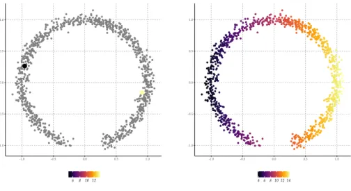
-1.0 -0.5 0.0 0.5 1.0

-1.0 -0.5 0.0 0.5 1.0

6 8 1012

(a) Observed data

-1.0 -0.5 0.0 0.5 1.0

-1.0 -0.5 0.0 0.5 1.0

46 810 12 14

(b) Predictions

Figure 2 |Regression example where the unlabeled data could convince one to update the estimated function by assuming the two ends of arcs are more likely to have a value similar to objects that are close in the intrinsic geometry indicated by the unlabeled data.

when measured when only considering paths through high density areas.

Note that in both cases the labeled data do not tell us whether these assumptions that lead to changes to the decision boundary are true. We intuit them on top of the labeled information that is already there.

A second argument for the merit of unlabeled data is that humans also do not seem to learn in a strictly supervised way. Both children and adults do not require constant feedback when learning to recognize objects or improve their judgement. Zhu and Goldberg (2009, Ch.7) ofer an overview and discussion of some of the research in cognitive science that studies the question whether humans actually use unlabeled data to adapt their judgement. Results are mixed, but suggest that in simple experimental settings humans use semi-supervised learning to solve tasks. However, even if semi-supervised learning is used by humans as a heuristic in many of the practical problems nature throws at us, this does not necessarily mean that it is possible in general, nor does it clearly demarcate when semi-supervised learning has merit.

the need for safe semi-supervised learning 13

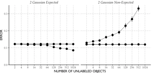
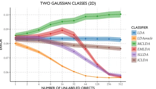
2 Gaussian Expected 2 Gaussian Non-Expected

2 4 8 16 32 64 128 256 512 1024 2 4 8 16 32 64 128 256 512 1024 0.0

0.1 0.2 0.3

NUMBER OF UNLABELED OBJECTS

ERROR

Supervised Self-learning

Figure 3 |Example where semi-supervised learning improves performance (left) and re-duces performance (right) as compared to the supervised alternative.

Pang, 2003; Patel and Wang, 2015), nuclear power plant monitoring (Ma and Jiang, 2015; Moshkbar-bakhshayesh and Ghofrani, 2016), food quality (Dean et al., 2006) and remote sensing (Gómez-Chova et al., 2008), among other applications. For instance, promising results in computer vision are shifting interest to leveraging abundant unlabeled data (Rasmus et al., 2015).

The Need for Safe Semi-supervised Learning

we observe in supervised classiiers, where we generally ind that adding labeled data increases classiication performance, regardless of misspeciication. For some exceptions to this general behaviour, see, for instance (Loog and Duin, 2012).

Arguments for the Limitations of SSL

Given these negative results, one could argue that it is a priori unlikely that ex-amples of the input alone will tell us anything at all about the outcome given the input. How, for instance, does knowing a certain percentage of web pages have the word ‘model’ in it tell us anything about the probability that a page is about ‘fashion’ or ‘statistics’ given that it contains the word ‘model’?

Seeger (2001) argues that for discriminative models where we directly model

pY_|X(which he calls the diagnostic paradigm), semi-supervised learning is impossible

unless one can make useful assumptions about the relationship between the para-meters governing the distribution that generates the input valesXand the

distri-bution that generates the labelsYgiven someX = x. His argument can be

illus-trated by the graphical model in Figure 4(a). The parametersθX, corresponding

to the data generating distribution ofX, andθ_Y|X, corresponding to the data

gen-erating distribution ofY given X, are a priori independent. Because of the way

the likelihood factorizes, unlabeled data play no role in updating beliefs aboutθ_Y|X

and additionally, learning something aboutθX should not inluence our estimate

ofθY|X. Compare this to the generative model in Figure 4(b), whereθX andθY|X

are dependent if we observeX.

Hansen (2009) makes a related argument by constructing the optimal Bayesian predictor for the squared loss, given that we know the prior that nature uses over parameters to generate datasets. He inds that in general this optimal predictor is given by the following solution:

∫ ∫

yp(y|x,θ)dy∫ p(x,Dl,Du|θ)p(θ) p(x,Dl,Du|θ′)p(θ′)dθ′

dθ,

whereDlis the labeled data set andDuis the unlabeled dataset andp(θ)is the true

prior on the parameters that is used by nature to generate datasets. Now suppose we split the parameter vector θ into three sets, one belonging to the conditional

distributionpY|X, one belonging to pX and one that is shared between these two.

When this shared set is empty, the optimal solution becomes:

∫ ∫

yp(y|x,θ)dy∫ p(Dl|θ)p(θ) p(Dl|θ′)p(θ′)dθ′

dθ.

arguments for the limitations of ssl 15

If these models correspond exactly to the data generating process, then these ar-guments hold. Yet these arar-guments do not tell us anything about the model itself: what are the possibilities of these models if, for instance, the dependence relation-ships between the variables are diferent from what the model assumes? Schölkopf, Janzing et al. (2012) consider this situation more explicitly, by also assuming causal semantics for the models using structural causal models to describe them. They show that indeed, in the model described in Figure 4(a), semi-supervised learning can not outperform supervised learning. The main concept in their analysis is that of the causal direction of prediction. IfXis the input,Y the output we are

inter-ested in predicting and Figure 4(a) is a representation of the causal structure of the problem, then we are predicting in the causal direction and semi-supervised learning is impossible, due to so-calledindependence of mechanism. This is assum-ing there are no other confoundassum-ing variables. On the other hand, if the true causal model is represented by Figure 4(b), we are in the anti-causal prediction scenario and information aboutpXis informative about thepY_|X.

Summarizing, these arguments depend on the assumption that the models cor-respond to the true data generating process but tell us little about the possibilities of unlabeled data for a method for which this correspondence is not correct. In practice, however, we often deal with, non-Bayesian, potentially misspeciied mod-els and inite amounts of data. Even if unlabeled data are not informative for the true model, this does not guarantee it might not be useful to improve estimates for models used or for inite amounts of data: they may, for instance, suggest what part of the feature space is best served by more accurate predictions from a model with limited complexity.

For example, Sokolovska et al. (2008) show that for logistic regression with dis-crete input features, if the model is misspeciied, information aboutpXis

informat-ive and leads to an estimator with lower asymptotic variance than the supervised estimator. All in all, model misspeciication and inite sample sizes seem to play an under appreciated role in these graphical model analyses of the semi-supervised problem.

Ben-David, Lu et al. (2008) take a learning theory approach to identify the use-fulness of unlabeled data in the “no prior knowledge” setting, meaning the setting where we do not make assumptions about the link between pY|X and pX. They

show that for some simple concept classes over the real line, algorithms that use unlabeled data can not give sample size guarantees that are more than a constant factor better than supervised algorithms. Sample size guarantees are guarantees that the algorithm will make an error of at most ϵwith probabilityδfor a given

ap-X Y

θX θY|X

(a) Diagnostic Model

X Y

θ_X|Y θY

(b) Generative Model

Figure 4 |Graphical model representations of two modelling paradigms. When assum-ing causal semantics and Y as beassum-ing the outcome of interest, (a) is an example of prediction in the causal direction, while (b) is prediction in the anti-causal direction.

proaches is that it is untestable and give examples when these assumptions can lead to deteriorated performance compared to supervised empirical risk minimization. The general consensus from these analyses is that unlabeled data will not lead to improved performance unless there is a link betweenpXandpY|X. Most of these

analyses, however, depend on the assumption that the model is correctly speciied or depend on asymptotic arguments. In practice, our model will not perfectly it the data and we have a limited number of observations. Moreover, even though some results suggest that semi-supervised learning without assumptions is only possible when the model is misspeciied, this is exactly the situation where semi-supervised learning might fail. Can we instead consider whether semi-supervised learning is possible based on the properties of the method, rather than the data generating process and can we guarantee that improvement happens in a safe way in a setting where we have limited data?

Assumptions We Might Need

While the research covered so far does still not fully characterize the possibilities of semi-supervised learning in the general case, many authors suggest that assump-tions are needed that link knowledge about pX to knowledge about pY|X. Let us

assumptions we might need 17

make such assumptions.

A classic analysis by Castelli and Cover (1995) shows that if we assume identi-iable mixture models where each component of the mixture belongs to one class, and we have an ininite amount of unlabeled samples, a single labeled sample gives a classiication risk of2R∗(1−R∗), withR∗being the minimum attainable

classiic-ation error. Adding more labeled examples allows convergence to this Bayes error with rate:

R(Nl,Nu =∞)−R∗=exp(−lK+o(l)),

withK being a measure of similarity between the class conditional distributions.

The idea behind this analysis is that the unlabeled data will identify the diferent decision regions, while the labeled data only have to be used to identity which de-cision region belongs to which class.

This may suggest labeled data are exponentially more valuable than unlabeled data, but note the exponential value comes after we used the ininite amount of un-labeled data. Castelli and Cover (1996) extend this analysis to the inite sample case, for a simpler situation where we either know the class conditional distribution for each class and only need to estimate the class prior or we know the class condition-als but not the assignment of class conditioncondition-als to classes. In the former case, the value of examples in reducing the risk is proportional to the Fisher information of the labeled and unlabeled data, where the value of the labeled data are strictly lar-ger than the unlabeled data. In the second scenario, a diference in the value of both types of information can also be shown to hold, although in this case, no learning is possible without labeled examples.

An important aspect highlighted in these analyses is that the role the unlabeled data play is in reducing the number of possible decision functions, between which we can then eiciently ind the correct one with limited labeled data. This idea is used in many of the following analyses as well.

Laferty and Wasserman (2007) consider the utility of the assumption of smooth-ness, where one assumes a regression function is smooth in regions wherepX(x)

is high. They ind that the manifold assumption (see below) alone is suicient, but that a class of algorithms that attempts to use the manifold and smoothness as-sumptions together do not ofer better convergence rates in terms of the squared error than supervised procedures. They do construct, however, new approaches that use either of these assumptions individually that do have improved conver-gence rates by using the unlabeled data.

ap-proximation error converges to zero at a fast rate. At the same time, for this class of problems, there is no supervised algorithm for which convergence can be guaran-teed for all distributions in the class. The intuition behind why knowledge of the manifold will help identify the correct conditional distribution is that it reduces the space of potential solutions, after which regular convergence results guarantee fast convergence.

Similarly, Singh et al. (2008) apply minimax lower bounding techniques to a version of the cluster assumption, where outcomes or conditional distributions are assumed to be smooth within a cluster, or decision set. They show that if these decision sets can be found using the unlabeled data and if a supervised learner with knowledge of these sets outperforms one without this knowledge, gathering unlabeled samples at a fast enough rate guarantees improved performance. Us-ing a speciic regression scenario, they show how the merit of unlabeled examples depends strongly on the margin between the decision sets and the amount of un-labeled data.

Based on the potential of semi-supervised methods to decrease performance compared to supervised procedures, Li and Zhou (2015) construct a safe version of the semi-supervised support vector machine by employing a low-density separ-ation assumption. The assumption is that the true decision boundary is situated in regions of low-density in the feature space. The idea behind this approach is to generate a set of low-density separators and pick one conservatively. If indeed this set contains the true solution, they are able to show procedure will improve in terms of performance compared to the supervised procedure.

In summary, given that we can make assumptions that linkpXandpY|X, it is

pos-sible to prove unlabeled data have some value. But as Ben-David, Lu et al. (2008) and others have pointed out, checking these assumptions is often diicult or im-possible. If we can not be sure these assumptions are true and the unlabeled data may lead to a procedure with reduced performance, perhaps we should avoid them completely. The view taken in this thesis is then to forego these assumptions, and ind out whether semi-supervised learning is still possible for this case and what performance guarantees this allows us to derive.

research questions 19

Research Questions

Based on these considerations, the main questions that we will address in this thesis are the following:

• Can we construct a (non-trivial) semi-supervised version of some supervised classiier without making additional assumptions that were not inherent in the supervised method?

• For these classiiers, in what sense can we guarantee that they (safely) improve over the supervised alternative?

• Can we prove this notion of safe semi-supervised learning is (im)possible for other classiiers?

During these investigations, some additional questions will come up that we try to address. For instance, why do semi-supervised approaches applied to the unreg-ularized least squares classiier fail when the dimensionality of the input sample is larger than the size of the sample? And what is a proper deinition for self-learning approaches to the least squares classiier that may not work in all cases, but give decent performance in many cases?

To answer these and other questions, we will rely on both mathematical analalysis as well as results from computational simulations and experiments. What is the role of reproducibility of these experiments in pattern recognition research and how do we ensure it?

Important Conceptual Constructs

Before continuing with the outline of the thesis, we will cover some of the most important concepts in the thesis that we will use to address the research question, which may help put things in perspective.

Surrogate losses

The lossLthat is optimized in the ERM framework outlined above, does not

Margin-based Losses

One particular class of these losses are so-called margin-based losses. These are losses of the formϕ(y f(x))wherey∈ {−1,+1}is the encoding of the binary class

label. Margin-based losses have been studied extensively in the context of their convergence properties. Bartlett et al. (2006), for instance, show that for any convex

ϕwithϕdiferentiable at0and ϕ′(0) < 0thenϕisclassiication calibrated, which implies that if a sequence of measurable functions converges to the optimal risk in terms of this margin-based loss, this sequence also converges to the Bayes risk in terms of classiication error (Bartlett et al., 2006, Theorem 1.3c). Various well-known and often used classiication methods can be formulated as the risk minimization of some margin-based loss, such as support vector machines, forms of boosting, logistic regression and the least squares classiier.

On Squared Loss

The least squares classiier can be deined as the decision function that minimizes the squared loss on the training data. For linear classiiers, one could also interpret this as encoding the vector of class labels as a numeric vector and using this as the dependent variable in linear regression.

In this thesis we consider the squared loss extensively. One could argue, how-ever, that this loss is antiquated, unsuitable or somehow non-optimal for classiic-ation (Ben-David, Loker et al., 2012). Yet the squared loss shares many properties with other commonly used loss functions. For instance, it is a margin-based loss and it is classiication calibrated (see above). Moreover, as many have observed, empirically it gives similar performance in terms of the error rate as other losses on many example datasets (Rifkin et al., 2003; Poggio and Smale, 2003; Zhang and Peng, 2004; Rasmussen and Williams, 2005). Rifkin (2002) even notes that “the choice between SVM and RLSC [regularized least squares classiier] should be based on computational tractability considerations”. One particular advantage of the squared loss is that it leads to a closed-form solution of the classiier which makes it easier to analyse theoretically, a property we will make use of repeatedly throughout the thesis.

Projected Estimators

important conceptual constructs 21

Projecting estimators onto sets of constraints has been considered for other prob-lems in statistics. For instance, the case where one knows the true solution adheres to certain linear inequality constraints (Schmidt and Stahlecker, 1995; Schmidt, 1996) or constraints that form some convex set (Stahlecker et al., 1996). Schmidt and Stah-lecker (1995) prove, for example, that the projection of any estimator to the set of linear inequality constraints leads to an equal or improved estimator: one that is ‘closer’ to the true solution and dominates the non-projected estimator, given that the true solution is within the set of constraints.

In the setting considered in our work, however, we do know such constraints, all we have is labeled and unlabeled objects. How, then, can we apply these projections to the semi-supervised setting? More speciically:

1. What is the estimator that is to be projected? 2. How do we form the constraint set?

3. How do we measure what it means for solutions to be ‘close’? 4. How do we choose a solution from the constraint set?

As we will elaborate in the rest of this thesis, in our semi-supervised solutions, we propose the following answers to these questions: (1) The solution to be projected is the supervised solution. (2) The constraint set is formed implicitly by all possible supervised classiiers we could get by assigning a potential labeling to the unlabeled objects. (3) The measure depends on the loss we are interested in minimizing and (4) we ind the semi-supervised solution either through minimizing the supervised loss within the constraint set (Chapters 1 and 2) or minimizing a particular distance measure that ensures we always get a better estimator (Chapter 3).

-1 0 1 2

-2 0 2

X

CLA

SS

Figure 5 |Dataset used to illustrate the projection example that corresponds to the pro-jection illustrated on the cover of the thesis. The circles indicate the locations and labels of the two labeled objects. The solid line indicates the supervised de-cision function, while the dashed lines correspond to the locations of the two unlabeled objects

the semi-supervised solution is always better than the supervised solution, as we will show in Chapter 3.

A Map but not the Territory

a map but not the territory 23

classiier, linear discriminant analysis, to show how the approach extends to other classiiers.

While the approach in Chapter 1 is guaranteed to improve over the supervised learner in a very restricted setting, in Chapter 3 we extend these results to the more general multivariate setting for a diferent, but related, procedure. We interpret this procedure as a projection of the supervised solution onto the implicit constraints set. For a particular distance measure we can then prove this procedure is always better than the supervised solution when evaluated in terms of the surrogate loss on the labeled and unlabeled data.

Since these performance guarantees are in terms of the surrogate loss, instead of the classiication error or some other common performance measure, in part two of the thesis, we consider the importance of these surrogate losses. In Chapter 4, we discuss situations in which it is insightful to consider the surrogate loss to study the behaviour of classiiers. In Chapter 5, we consider these surrogate losses to prove for a particular class of classiiers based on margin-based losses that under certain conditions, safe semi-supervised learning is impossible. We also show for which cases improvement guarantees are possible, covering, among other cases, the results we obtained in Chapter 3.

In Chapter 6, we turn away from the pessimism considered in Chapter 3 to con-sider how to properly deine an optimistic version of the least squares classiier. We show how to deine a soft-label self-learning variant of the least squares classiier and study its properties.

In Chapter 7, then, we cover the peaking phenomenon in semi-supervised learn-ing, that we ran into during some of the experiments in this thesis and which was briely covered in Chapter 1. We show, for a simple semi-supervised least squares approach, where this behaviour originates and why it is more extreme than in the supervised setting.

The inal part of this thesis, part three, is devoted to questions concerning the re-producibility of the results of the rest of the thesis. Chapter 8 discusses the concepts of reproducibility and replicability in the pattern recognition context and ofers a case study of reproducing Chapter 6, as well as additional results. Chapter 9 de-scribes the toolbox we implemented to produce all the results in this thesis, that can be used to reproduce these and other results in semi-supervised learning re-search.

CONSTRAINTS & PROJECTIONS

CHAPTER ONE

Implicitly Constrained Semi-supervised

Least Squares Classiication

We introduce the implicitly constrained least squares (ICLS) classifier, a novel semi-supervised version of the least squares classifier. This classifier minimizes the squared loss on the labeled data among the set of parameters implied by all possible labelings of the unlabeled data. Unlike other discriminative semi-supervised methods, this ap-proach does not introduce explicit additional assumptions into the objective function, but leverages implicit assumptions already present in the choice of the supervised least squares classifier. This method can be formulated as a quadratic programming problem and its solution can be found using a simple gradient descent procedure. We prove that, in a limited one dimensional setting, this approach never leads to performance worse than the supervised classifier. Experimental results show that also in the general multidimensional case performance improvements can be expected, both in terms of the squared loss that is intrinsic to the classifier, as well as in terms of the expected classification error.

1.1 Introduction

We consider the problem of semi-supervised learning of binary classiication func-tions. As in the supervised paradigm, the goal in semi-supervised learning is to construct a classiication rule that maps objects in some input space to a target out-come, such that future objects map to correct target outcomes as well as possible. In

This chapter appeared as: Krijthe, J.H. & Loog, M., 2017. Robust Semi-supervised Least Squares Classi-ication by Implicit Constraints. Pattern Recognition, 63, pp.115–126. An earlier, shorter, version of this work appeared as: Krijthe, J. H., & Loog, M. (2015). Implicitly Constrained Semi-Supervised Least Squares Classiica-tion. In E. Fromont, T. De Bie, & M. van Leeuwen (Eds.), Advances in Intelligent Data Analysis XIV. Lecture Notes in Computer Science, vol 9385. (pp. 158–169).

the supervised paradigm this mapping is learned using a set ofLtraining objects

and their corresponding outputs. In the semi-supervised scenario we are given an additional and often large set ofU unlabeled objects. The challenge of

semi-supervised learning is to incorporate this additional information to improve the classiication rule.

The goal of this work is to build a semi-supervised version of the least squares classiier that is robust against deterioration in performance meaning that, at least in expectation, its performance is not worse than supervised least squares classi-ication. While it may seem like an obvious requirement for any semi-supervised method, current approaches to semi-supervised learning do not have this property. In fact, performance can signiicantly degrade as more unlabeled data is added, as has been shown in (Cozman and Cohen, 2006; Cozman, Cohen and Cirelo, 2003), among others. This makes it diicult to apply these methods in practice, especially when there is a small amount of labeled data to identify possible reduction in per-formance. A useful property of any semi-supervised learning procedure would therefore be that its performance does not degrade as we add more unlabeled data. Additionally, many semi-supervised learning procedures are formulated as hard-to-optimize, non-convex objective functions. A more satisfactory state of afairs for semi-supervised classiication would therefore be methods that are easier to train and that, on average, do not lead to worse classiication performance than their supervised alternatives.

We present a novel approach to semi-supervised learning for the least squares classiier that we will refer to as implicitly constrained least squares classiication (ICLS). ICLS leverages implicit assumptions present in the supervised least squares classiier to construct a semi-supervised version. This is done by minimizing the su-pervised loss function subject to the constraint that the solution has to correspond to the solution of the least squares classiier for some labeling of the unlabeled ob-jects.

As this work is speciically concerned with least squares classiication, we note several reasons why this is a particularly interesting classiier to study: First of all, the least squares classiier is a discriminative classiier. Some have claimed semi-supervised learning without additional assumptions is impossible for discrimin-ative classiiers (Seeger, 2001; Singh et al., 2008). Our results show this does not strictly hold.

Secondly, the closed-form solution for the supervised least squares classiier al-lows us to study its theoretical properties. In particular, in the univariate setting without intercept and assuming perfect knowledge ofPX, the distribution of the

quad-1.2. related work 29

ratic programming problem, which can be solved through a simple gradient des-cent with boundary constraints.

Lastly, least squares classiication is a useful and adaptable classiication tech-nique allowing for straightforward use of, for instance, regularization, sparsity pen-alties or kernelization (Hastie et al., 2009; Poggio and Smale, 2003; Rifkin et al., 2003; Suykens and Vandewalle, 1999; Tibshirani, 1996). Using these formulations, it has been shown to be competitive with state-of-the-art methods based on loss functions other than the squared loss (Rifkin et al., 2003) as well as computation-ally eicient on large datasets (Bottou, 2010).

This work builds on (Krijthe and Loog, 2015) and ofers a more complete expos-ition: we show ICLS can be formulated as a quadratic programming problem, we extend the experimental results section by including an alternative semi-supervised procedure, adding additional datasets and discussing the ‘peaking’ phenomenon. Moreover, we extend the theoretical result with conditions when one is likely to see improvement of the proposed approach over the supervised classiier.

The main contributions of this paper are

• A novel convex formulation for robust semi-supervised learning using squared loss (Equation 1.5)

• A proof that this procedure never reduces performance in terms of the squared loss for the 1-dimensional case without intercept (Theorem 1)

• An empirical evaluation of the properties of this classiier (Section 1.6) The rest of this paper is organized as follows. Section 1.2 gives an overview of related work on semi-supervised learning. Section 1.3 gives a high level overview of the method while Section 1.4 introduces our semi-supervised version of the least squares classiier in more detail. We then derive a quadratic programming formu-lation and present a simple way to solve this problem through bounded gradient descent. Section 1.5 contains a proof of the improvement of the ICLS classiier over the supervised alternative. This proof is speciic to classiication with a single fea-ture, without including an intercept in the model. For the multivariate case, we present an empirical evaluation of the proposed approach on benchmark datasets in Section 1.6 to study its properties. The inal sections discuss the results and con-clude.

1.2 Related Work

(Shi and Zhang, 2011), it has also been observed that these techniques may give per-formance worse than their supervised counterparts. See for instance (Cozman and Cohen, 2006; Cozman, Cohen and Cirelo, 2003), for an analysis of this problem, and (Elworthy, 1994) for a practical example in part-of-speech tagging. In these cases, disregarding the unlabeled data would lead to better performance.

Some (Goldberg and Zhu, 2009; Wang, Shen and Pan, 2007) have argued that agnosticsupervised learning, which Goldberg and Zhu (2009) deines as semi-supervised learning that is at least no worse than semi-supervised learning, can be achieved by cross-validation on the limited labeled data. Agnostic semi-supervised learn-ing follows if we only use semi-supervised methods when their estimated cross-validation error is signiicantly lower than those of the supervised alternatives. As the results of Goldberg and Zhu (2009) indicate, this criterion may be too conser-vative: given the small amount of labeled data, a semi-supervised method will only be preferred if the diference in performance is very large. If the diference is less distinct, the supervised learner will always be preferred and we potentially ignore useful information from the unlabeled objects. Moreover, this cross-validation ap-proach can be computationally demanding.

Self-Learning

A simple approach to semi-supervised learning is ofered by the self-learning pro-cedure (McLachlan, 1975) also known as Yarowsky’s algorithm (see (Abney, 2004) and (Yarowsky, 1995)) or retagging (Elworthy, 1994). Taking any classiier, we irst estimate its parameters on only the labeled data. Using this trained classiier we label the unlabeled objects and add them, or potentially only those we are most conident about, with their predicted labels to the labeled training set. The classi-ier parameters are re-estimated using these labeled objects to get a new classiclassi-ier. One iteratively applies this procedure until the predicted labels of the unlabeled data no longer change.

1.2. related work 31

Additional Assumptions

Some semi-supervised methods leverage the unlabeled data by introducing assump-tions that link properties of the features alone to properties of the label of an object given its features. Commonly used assumptions are the smoothness assumption: objects that are close in the feature space likely share the same label; the cluster as-sumption: objects in the same cluster share a label; and the low density assumption enforcing that the decision boundary should be in a region of low data density.

The low-density assumption is used in entropy regularization (Grandvalet and Bengio, 2005) as well as for support vector classiication in the transductive sup-port vector machine (TSVM) (Joachims, 1999) and closely related semi-supervised SVM (S3_{VM) (Bennett and Demiriz, 1998; Sindhwani and Keerthi, 2006). In these}

approaches an additional term is added to the objective function to push the de-cision boundary away from regions of high density. Several approaches have been put forth to minimize the resulting non-convex objective function, such as the con-vex concave procedure (Collobert et al., 2006) and diference concon-vex programming (Sindhwani and Keerthi, 2006; Wang and Shen, 2007).

In all these approaches to semi-supervised learning, a parameter controls the importance of the unlabeled points. When the parameter is correctly set, it is clear, as Wang, Shen and Pan (2007) claims, that TSVM is always no worse than super-vised SVM. It is, however, non-trivial to choose this parameter, given that semi-supervised learning is most interesting in cases where we have limited labeled ob-jects, making a choice using cross-validation very unstable. In practice, therefore, TSVM can also lead to performance worse than the supervised support vector ma-chine, as well will also see in Section 1.6.

Safe Semi-supervised Learning

Aside from the work by Loog (2010) and Loog and Jensen (2014), another at-tempt to construct a robust semi-supervised version of a supervised classiier has been made in (Li and Zhou, 2011), which introduces the safe semi-supervised sup-port vector machine (S4_{VM). This method is an extension of S}3_{VM (Bennett and}

Demiriz, 1998) which constructs a set of low-density decision boundaries with the help of the additional unlabeled data, and chooses the decision boundary, which, even in the worst-case, gives the highest gain in performance over the supervised solution. If the low-density assumption holds, this procedure provably increases classiication accuracy over the supervised solution. The main diference with the method considered in this paper, however, is that we make no such additional as-sumptions. We show that even without these assumptions, safe improvements are possible for the least squares classiier.

Semi-supervised Least Squares

While least squares classiication has been widely used and studied (Hastie et al., 2009; Poggio and Smale, 2003; Suykens and Vandewalle, 1999), little work has been done on applying semi-supervised learning to the least squares classiier speciic-ally. For least squares regression, Little and Rubin (2002) describe an iterative method for handling missing outcomes that was formally proposed by Healy and Westmacott (1956). In the case of least squares regression, this method has some computational advantages over discarding the unlabeled data but its solution al-ways coincides with the supervised solution. Shafer (1991) studied the value of knowingE_[XT_X], where_Xis the_L×ddesign matrix containing the feature values

for each observation. If we assume the number of unlabeled data points is large, this is similar to the semi-supervised situation. It is shown that if the size of the parameters is small compared to the noise, the variance of a procedure that plugs inE_[XT_X]as the estimate of_XT_Xhas a lower variance than supervised least squares

regression. As the size of the parameters increases, this efect reverses. In fact, the paper demonstrates that in this semi-supervised setting no best linear unbiased estimator for the regression coeicients exists. In Section 1.6, we compare our ap-proach to using this plug-in estimate by substituting the matrixXTXby a version

based on both labeled and unlabeled data. A similar plug-in procedure has been used by Fan et al. (2008) for linear discriminant analysis for dimensionality reduc-tion which is closely related to least squares classiicareduc-tion. Here the (normalized) total scatter matrix, which plays a similar role to theXTXmatrix in least squares

1.3. implicitly constrained least squares classification 33

1.3 Implicitly Constrained Least Squares Classiication

Given a limited set ofLlabeled objects and a potentially large set ofUunlabeled

objects, the goal of implicitly constrained least squares classiication is to use the latter to improve the solution of the least squares classiier trained on just the labeled data. We start with a sketch of this approach, before discussing the details.

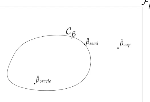
ˆ

β

C

_β

F

_β

ˆ

β

ˆ

β

Figure 1.1 |A visual representation of implicitly constrained semi-supervised learning._Fβ is the space of all linear models. _βˆ_supdenotes the solution given only a small amount of labeled data. _Cβ is the subset of the space which contains all the solutions we get when applying all possible (soft) labelings to the unlabeled data._βˆ_semiis the solution in_Cβthat minimizes the loss on the labeled objects.

ˆ

βoracleis the supervised solution if we would have the labels for all the objects.

Given the supervised least squares classiier, consider the hypothesis space of all possible parameter vectors, which we will denote asFβ, see Figure 1.1. Given a set

of labeled objects, we can determine the supervised parameter vector_βˆ_{sup. Suppose} we also have a potentially large numberUof unlabeled objects. Assume that every

object has a label, it is merely unknown to us. If these labels were to be revealed, it is clear how the additional objects can improve classiication performance: we es-timate the least squares classiier using all the data to obtain the parameter vector

ˆ

estim-ate to be better. These real labels are unknown, but we can still consider all pos-sible labelings of unlabeled objects, and estimate corresponding parameters based on these imputed labelings. In this way, we get a set of possible parameters for our classiier, which form the set denoted byCβ ⊂ Fβ. Clearly one of these labelings

corresponds to the real, but unknown, labeling, so one of the parameter estimates in this set corresponds to the solution we would obtain using all the correct labels of both the labeled and unlabeled objects. Because these are the only possible clas-siiers when the true labels would be revealed, we propose to look within this set

Cβfor an improved semi-supervised solution.

Two issues then remain: how do we choose the best parameters from this set and how do we ind these without having to enumerate all possible labelings?

Looking at the irst problem, we reiterate that the goal of semi-supervised learn-ing is to ind a good classiication rule and, therefore, still the obvious way to evalu-ate this rule is by the loss on the labeled training points. In other words, we choose the classiier from the parameter set that minimizes the squared loss on the labeled points. We will denote this solution by_βˆ_{semi. Note this approach is rather diferent} from other approaches to semi-supervised learning where the loss is adapted by including a term that depends on the unlabeled data points. In our formulation, the loss function is still the regular, supervised loss of our classiication procedure. As for the second issue, after relaxing the constraint that we need hard labels for the data points, we will see that the resulting optimization problem is, in fact, an instantiation of well-studied quadratic programming, which we solve using a simple gradient descent procedure.

1.4 Method

Supervised Multivariate Least Squares Classiication

Least squares classiication (Hastie et al., 2009; Rifkin et al., 2003) is the direct ap-plication of well-known ordinary least squares regression to a classiication prob-lem. A linear model is assumed and the parameters are minimized under squared loss. LetXbe anL×(d+1)design matrix withLrows containing vectors of length

equal to the number of featuresdplus a constant feature to encode the intercept.

Vectorydenotes anL×1vector of class labels. We encode one class as0and the other as1. The multivariate version of the empirical risk function for least squares estimation is given by

ˆ

R(β) = 1

L∥Xβ−y∥

2

1.4. method 35

The well-known closed-form solution for this problem is found by setting the de-rivative with respect toβequal to0and solving forβ, giving

ˆ

β=(XTX)−1XTy. (1.2)

In caseXTXis not invertible (for instance whenL < (d+₁)), a pseudo-inverse is applied. As we will see, the closed form solution to this problem will enable us to formulate our semi-supervised learning approach in terms of a standard quadratic programming problem, which is easy to optimize.

Implicitly Constrained Least Squares Classiication

In the semi-supervised setting, apart from a design matrixXand target vector y,

an additional set of measurementsXuof sizeU×(d+1)withouta corresponding

target vector yu is given. In what follows, Xe = [XT XT_u]T denotes the

exten-ded design matrix which is simply the concatenation of the design matrices of the labeled and unlabeled objects.

In the implicitly constrained approach, we incorporate the additional informa-tion from the unlabeled objects by searching within the set of classiiers that can be obtained by all possible labelingsyu, for the one classiier that minimizes the

super-visedempirical risk function in Equation (1.1). This set,Cβ, is formed by theβs that

would follow from training supervised classiiers on all (labeled and unlabeled) ob-jects going through all possible soft labelings for the unlabeled samples, i.e., using allyu ∈ [0, 1]U_{. Since these supervised solutions have a closed form, this can be}

written as

Cβ:=

{

β=(X_eTXe)−1X_eT [

y yu

]

:yu∈[0, 1]U

}

. (1.3)

The soft labeling provides both a relaxation for computational reasons as well as a strategy to deal with label uncertainty. We can interpret these fractions as a type of class posterior for the unlabeled objects. This constraint setCβ, combined with

the supervised loss that we want to optimize in Equation (1.1), gives the following deinition for implicitly constrained semi-supervised least squares classiication:

argmin

β∈Cβ

ˆ

R(β). _(1.4)

Sinceβis ixed for a particular choice ofyuand has a closed form solution, we can

rewrite the minimization problem in terms ofyuinstead ofβ:

argmin

yu∈[0,1]U

1 L

X(XTeXe )−1

The problem deined in Equation (1.5) can be written in a standard quadratic pro-gramming form: min yu 1 2y T

uQyu+cTyu

subject to:

[ IU

−IU ]

yu≤

[ 1U 0U

] (1.6)

where1

Q=2 LXu

( XT_eXe

)−1

XTX(XT_eXe )−1

XT_u,

and

c=2 LXu

(

XT_eXe)−1XTX(XT_eXe)−1XTy

− 2

LXu

(

XT_eXe)−1XTy.

Here,IUdenotes theU×Uidentity matrix and1Uand0Udenote column vectors

of respectively ones and zeros.

Since the matrixQis a product of a matrix and its transpose, it is guaranteed

to be positive semi-deinite. The problem is typically not positive deinite because there are diferent labelings that will lead to one and the same minimum objective.

The quadratic problem deined above can be solved using, for instance, an in-terior point method. We have found a gradient descent approach to be easier to apply. Taking the derivative with respect toyuand rearranging the terms we ind

∂Rˆ ∂yu =

2

LXu

( X_eTXe

)−1

XTX(X_eTXe )−1

XTy

+ 2 LXu

( XT_eXe

)−1

XTX(XT_eXe )−1

XT_uyu

− 2

LXu

( XT_eXe

)−1 XTy.

Because of its convexity, this problem can be solved eiciently using a quasi-Newton approach that allows for the[0, 1]box bounds, such as L-BFGS-B (Byrd

et al., 1995). Solving foryugives a labeling that we can use to construct the

semi-supervised classiier using Equation (1.2) by considering the imputed labels as the labels for the unlabeled data.

1.5 Theoretical Results

We will examine this procedure by considering it in a limited, yet illustrative setting. In this case we will, in fact, prove that our procedure willnevergive a worse least

1.5. theoretical results 37

squares estimate than the supervised solution. Consider the case where we have just one featurex, a limited set of labeled instances and assume we know the

prob-ability density function of this feature fX exactly. This last assumption is similar

to having unlimited unlabeled data and is also considered, for instance, by Soko-lovska et al. (2008). We consider a linear model with no intercept: y = xβwhere y, without loss of generality, is set as0for one class and1for the other. For new data points, estimatesyˆcan be used to determine the predicted label of an object by using a threshold set at, for instance,0.5.

The expected squared loss, or risk, for this model is given by

R∗(β) =

∑

y∈{0,1}

∫ ∞

−∞(xβ−y)

2_f

X,Y(x,y)dx, (1.7)

where fX,Y = P(y|x)fX(x). We will refer to this as the joint density ofXandY.

Note, however, that this is not strictly a density, since it deals with the joint distri-bution over a continuousXand a discreteY. The optimal solutionβ∗is given by

theβthat minimizes this risk:

β∗ =argmin

β∈R

R∗(β). (1.8)

We will show the following result:

Theorem 1. Given a linear model in 1D without intercept,y = xβ, and fX known, the estimate obtained through implicitly constrained least squares always has an equal or lower risk than the supervised solution:

R∗(βˆsemi)≤R∗(βˆsup).

In particular, given1labeled sample, if fX,Yis continuous in the featureXwith bounded second moment and fX,Y(0, 1)>0, then

E_[R∗_(βˆ_semi)]<E_[R∗_(βˆ_sup)].

Proof. Setting the derivative of (1.7) with respect toβto0and rearranging we get

β =

(∫ ∞

−∞x

2_f X(x)dx

)−1

∑

y_∈{0,1}

∫ ∞

−∞xy fX,Y(x,y)dx (1.9)

=

(∫ ∞

−∞x

2_f X(x)dx

)−1∫ ∞

−∞x fX(x)_y

∑

∈{0,1_}

yP(y|x)dx (1.10)

=

(∫ ∞

−∞x

2_f X(x)dx

)−1∫ ∞

−∞x fX(x)

ˆ

β

sup

β

ˆ

semi

β

∗

Solution

Squared

Loss

Figure 1.2 |An example where implicitly constrained optimization improves performance. The supervised solution_βˆ_supwhich minimizes the supervised loss (the solid curve), is not part of the interval of allowed solutions. The solution that min-imizes this supervised loss within the allowed interval is _βˆ_semi. This solution is closer to the optimal solutionβ∗than the supervised solutionβˆsup.

In this last equation, since we assume fX(x)as given, the only unknown is the

functionE_[y|x], the expectation of the label_y, given_x. Now suppose we consider

every possible labeling of the unlimited number of unlabeled objects including frac-tional labels, that is, every possible function whereE_{[y|x] ∈ [0, 1]}. Given this

re-striction onE_[y|x], the second integral in (1.11) becomes a re-weighted version of

the expectation operation overx. By changing the choice ofE_[y|x]one can vary the

value of this integral, but it will always be bounded on an interval onR. It follows

that all possibleβ’s also form an interval onR, which is the constraint set_Cβ. The

optimal solution has to be in this interval, since it corresponds to a particular but unknownE_[y|x].

Using the set of labeled data, we can construct a supervised solution_βˆ_supthat minimizes the loss on the training set ofLlabeled objects (see Figure 1.2):

ˆ

βsup=argmin

β_∈R

L

∑

i=1

(xiβ−yi)2. (1.12)

Now, either this solution falls within the constrained region,_βˆ_{sup ∈ Cβ or not,} ˆ

βsup∈ C/ β, with diferent consequences:

1.5. theoretical results 39

is no reason to update our estimate. Therefore_βˆ_semi=βˆ_sup.

2. Alternatively, if_βˆ_{sup∈ C/ β, the solution is outside of the constrained region (as} shown in Figure 1.2): there is no possible labeling of the unlabeled data that will give the same solution as_βˆ_{sup. We then update theβto be theβwithin} the constrained region that minimizes the loss on the supervised training set. As can be seen from Figure 1.2, this will be a point on the boundary of the interval. Note that _βˆ_{semi is now closer toβ}∗ _{than β}ˆ_{sup. Since the true loss} function R∗(β)is convex and achieves its minimum in the optimal solution,

corresponding to the true labeling, the risk of our semi-supervised solution will always be equal to or lower than the loss of the supervised solution. Thus, the proposed update either improves the estimate of the parameter βor

it does not change the supervised estimate. In no case will the semi-supervised solution be worse than the supervised solution, in terms of the expected squared loss. This concludes the proof of the irst part of the theorem.

The last part of the theorem gives a general condition when, in expectation, our semi-supervised approach will outperform the supervised learner. Because_βˆ_semi will never be worse than _βˆ_{sup, to prove this we only need to show that for some} observation of a labeled point with positive fX,Y(x,y) > 0, the estimatedβˆsupis

outside of the intervalCβ, in which caseR∗(βˆsemi)<R∗(βˆsup).

If we observe an object labeled1with feature valuex, the corresponding

estim-ate_βˆ_{sup =} 1

x. Since the improvement in loss will only result if this estimate is not

in the constrained region, we need to show that

P(1

x ∈ C/ β,y=1)>0 . (1.13)

To do this, consider the bounds of the intervalCβ. These most extreme values

are obtained whenever all negative values ofxare assigned label0while the pos-itivex get labels1, or the other way around. From (1.11) and writingE_(X2_{) =} ∫∞

−∞x2fX(x)dxwe ind the interval is given by

Cβ=

[∫0

−∞x fX(x)dx

E_(X2₎ ,

∫∞

0 x fX(x)dx

E_(X2₎ ]

. (1.14)

Combining this with (1.13), we get the condition

P

(

E_(X2₎

∫0

−∞x fX(x)dx

<_x<₀∨₀<_x <

E_(X2₎

∫∞

0 x fX(x)dx ,y=1

)

>_{0 .} (1.15)

Since fX,Y is assumed to be continuous,E[X2] > 0, and the lower bound in this

0. The assumption of the continuity of fX,Y ensures that (1.15) holds whenever

fX,Y(0, 1) > 0. The property fX,Y(0, 1) > 0 is satisied by many distributions of

the data. The result, therefore, indicates, that in the case of1labeled sample im-provement is not only possible, but will occur in many cases. When we have mul-tiple labeled examples, this efect will likely become smaller. This makes sense: the more labeled data we have to estimate the parameter, the smaller the impact of the unlabeled objects will be.

1.6 Empirical Results

To study the properties of the proposed semi-supervised approach to least squares classiication, we compare how this approach fares against supervised least squares classiication without the constraints.

For comparison we include two alternative semi-supervised approaches and an oracle solution:

Self-Learning Using a simple procedure proposed by McLachlan (1975), among others, the supervised least squares classiier is updated iteratively by using its class predictions on the unlabeled objects as the labels for the unlabeled objects in the next iteration. This is done until convergence.

Updated Second Moment Least Squares (USM) In this approach we replace the second moment matrixXTXwith an appropriately scaled matrixXTeXe similar to

the estimator studied in (Shafer, 1991):

ˆ

β_USM=(_L+L_UXT_eXe )−1

XTy

whereXeandyare centered. This centering ensures that results do not depend on

the particular encoding of the labels used. We will refer to this as updated second moment least squares (USM) classiication.

Oracle The performance of the least squares classiier if all unlabeled objects were labeled as well. This serves as the unattainable upper bound on the performance of any semi-supervised learner.

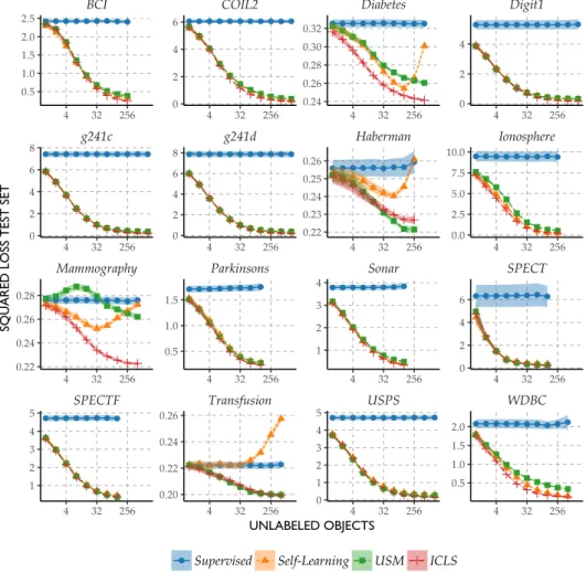
1.6. empirical results 41

the number of objects and features as well as the nature of the underlying prob-lems. Taken together, this collection allows us to investigate the properties of our approach for a wide range of problems. All the code used to run the experiments is available from the irst author’s website.

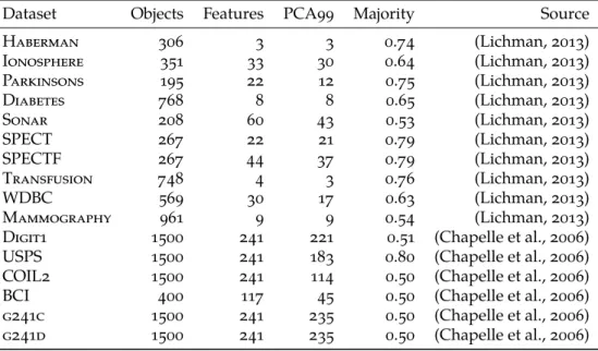
Table 1.1 |Description of the datasets used in the experiments. PCA99 refers to the number of principal components required to retain at least 99% of the variance. Majority refers to the proportion of the number of objects from the largest class

Dataset Objects Features PCA99 Majority Source

Haberman 306 3 3 0.74 (Lichman, 2013)

Ionosphere 351 33 30 0.64 (Lichman, 2013)

Parkinsons 195 22 12 0.75 (Lichman, 2013)

Diabetes 768 8 8 0.65 (Lichman, 2013)

Sonar 208 60 43 0.53 (Lichman, 2013)

SPECT 267 22 21 0.79 (Lichman, 2013)

SPECTF 267 44 37 0.79 (Lichman, 2013)

Transfusion 748 4 3 0.76 (Lichman, 2013)

WDBC 569 30 17 0.63 (Lichman, 2013)

Mammography 961 9 9 0.54 (Lichman, 2013)

Digit1 1500 241 221 0.51 (Chapelle et al., 2006) USPS 1500 241 183 0.80 (Chapelle et al., 2006) COIL2 1500 241 114 0.50 (Chapelle et al., 2006)

BCI 400 117 45 0.50 (Chapelle et al., 2006)

g241c 1500 241 235 0.50 (Chapelle et al., 2006) g241d 1500 241 235 0.50 (Chapelle et al., 2006)

Peaking Behaviour in Semi-supervised Least Squares

With fewer than d samples, thesupervised least squares classiier that utilizes a