List of Experiment
Subject: Physics Lab Subject code: EAS 151/ EAS 2511. To determine the wavelength of Sodium light by Newton’s ring.
2. To determine the wavelength of Sodium light with the help of Fresnel’s Biprism.
3. To determine the focal length of the combination of two thin convergent lenses separated by a distance with the help of a Nodal – Slide and verify to the formula.
4. To determine the specific rotation of cane sugar solution using Polarimeter.
5. To determine the wavelength of spectral lines using plane Transmission Grating.
6. To determine the specific resistance of a given wire using Carey Foster’s Bridge.
7. To study the variation of magnetic field along the axis of current carrying - Circular coil and then to estimate the radius of the coil.
8. To verify Stefan’s Law by Electrical Method.
9. To calibrate the given Ammeter and Voltmeter by potentiometer.
10. To determine the Energy Band Gap of a given semiconductor material.
11. To determine E.C.E. of copper using Tangent galvanometer.
12. To draw hysteresis curve of a given sample of ferromagnetic material and from - this to determine magnetic Susceptibility and permeability of the given specimen.
13. To determine the coefficient of viscosity of a Water.
14. To study the Hall Effect and determine Hall coefficient, carrier density and - mobility of a given semiconductor using Hall Effect set up.
15. Measurement of Wavelength of a laser (He- Ne) light using single slit diffraction.
Experiment Formula and Standard Result
1. Newton’s Ring λ Standard value = 5893 Å
3. Nodal Slide 2 1 2 1 1 1 1 f f x f f
F f f x
f f F 2 1 2 1
Standard value =20&25cm;F=12-13 cm
4. Polarimeter S = = Standard value=
5. Transmission Grating λ = Standard value= V-4047Å,G-4916Å,R-6908Å
6. Carey foster’s Bridge. X = Specific resistance of the wire Standard value
7. Variation of Magnetic Field tan
) ( 10 2 2 / 3 2 2 7 2 H x a i na
Standard value =
8.Stefan’s Law Standard value =
9A. Galvanometer into an Ammeter G = Ω, K = Amp. / div., Ig = nk, S= L =
Standard value =
9B. Galvanometer into a Voltmeter G = Ω, K = Amp. / div. Ig = nk, R =
–G
Standard value =
10. Energy Band Gap ρ0 = , ρ =
Eg = 2K × ; Eg = 2K × 2.303 × × 1000; Eg = 4.606 × 8.6 ×10-5× × 1000
Eg = 0.396 × ev Standard value =
11. Electro – Chemical Equivalent Z = Standard value =
12. Hysteresis Curve (B-H curve)
(a) Coercivity: × Loop width = ---mm H =
(b) Saturation magnetization: ( )s = × tip to tip height =---mV
= =
(c) Retentivity: ( )r = × (2 × Intercept) = =
(d) Magnetic Permeability: μ = = Slop of B – H curve
MAHARAJA AGARSAIN INSTITUTE OF TECHNOLOGY
PHYSICS PRACTICAL
INDEX
S.No. Name
1. List of experiment -
2. Index -
3. Instructions for Laboratory -
4. General Instructions -
5. Safety Rules -
6. Model Practical Record -
Experiments Page No.
1. Newton’s Ring 1-4
2. Fresnel’s Bi-Prism 5-9
3. Nodal Slide 10-15
4. Polarimeter 16-18
5. Transmission Grating 19-23
6. Carey Foster’s Bridge 24-27
7. Variation of magnetic field 28-31
8. Stefan’s Law 32-35
9. Calibration of a Voltmeter with a potentiometer 36-39
10. Calibration of a Ammeter with a potentiometer 40-43
11. Energy Band Gap 44-48
12. E.C.E of copper 49-51
13. Hysteresis curve 52-57
14. Viscosity of water 58-60
15. Hall Effect 61-66
16. Laser (He-Ne) light using Single slit diffraction 67-68
17 Polarization of light by simple reflection using laser
69-70
Experiment No. 1
To determine the wavelength of sodium light by measuring the diameter of Newton’s ring.
APPARATUS:
A Traveling microscope, a sodium lamp, Newton’s rings apparatus consisting of an optically plane glass plate and a convex lens of large focal length placed in a box having an optically plane glass plate inclined at an angle 450, a convex lens of short focal length etc.
PRECAUTIONS:
1. The lens and glass plate should be clean.
2. A lens of a large radius of curvature should be used.
3. The point of intersection of the cross-wires should coincide with the center of the ring system.
4. The micrometer screw should always be moved in the same direction to avoid error due to back-lash.
5. The radius of curvature of surface of the lens in the contact with glass plate should be measured accurately.
6. The amount of light from the source should be adjusted for maximum visibility. To much light increase the general illumination and decreases the contrast between bright and dark rings.
THEORY:
Circular interference fringes produced by enclosing a very thin air film of varying thickness between the surface of convex lens of a large radius of curvature and a plane glass plate are known as Newton’s ring.
In order to produce these fringes light from an extended monochromatic source S is rendered parallel by convex lens L. It falls on the glass plate G inclined at an angle of 450 to the vertical and is reflected normally on to the lens N. An air film of varying thickness is thus enclosed between the lower surface of this lens and the glass plate P. The light reflected from the upper and the lower surfaces of the air film produces interference fringes. At the center the lens is in contact with glass plate and thickness of the air film is zero. The centers will be dark as a phase change of is introduced due to reflection at the lower surface of the air film. As we proceed outward from the centre the thickness of the air film gradually increases being the same all along circle with centre at the point of contact. Hence the fringes produced are film. The fringes are viewed by means of a low power microscope M as show in fig1.
If R is the radius of curvature of the surface of the lens in contact with the glass plate P, Dn the diameter of the nth dark ring and λ the wavelength of light, then
D2n = 4nR λ
If the lens and the plate are not quite in contact at the centre of the ring system, as may occur if the surfaces are not clean, the centre may not be dark. To eliminate the error due to this the diameter of any two dark rings say nth and mth is determined, thus:
D2n= 4nR λ
And D2m = 4mR λ m < n
This formula involves the difference of the square of the diameter of the two rings and is independent of the thickness of the air film at the so called point of contact.
Fig. 1 Experimental arrangement for newton’s ring
PROCEDURE:
1. Level the microscope table and set the microscope tube in the vertical position. Find the vernier constant of the horizontal scale.
2. Clean the surface of the glass plate P, the lens N and the plate G. Place them in potion as show in the fig.1. Place the arrangement in front of a sodium lamp show that the height of the center of the glass plate G is the same as that of the center of the sodium lamp, placed in a wooden box having a hole of about one inch square in it at the same height. Place the convex lens in front of hole and adjust its position so that a parallel beam of light is made to fall on the glass plate inclined at an angle of 450.
3. Adjust the position of the microscope so that its lies vertically above the center of the lens N. Focus the microscope, so that alternate dark and bright rings are clearly visible.
4. Adjust the position of the microscope until the point of the inter-section of the cross-wire coincides with the center of the ring system and one of the cross-wire is perpendicular to the horizontal scale.
5. Slide the microscope to the left till the cross-wire lies tangentially at the 20th dark ring. The position of the cross-wire when the microscope is focused on 10th dark ring is shown in fig.2. Note the reading on the main scale and vernier scale of the microscope. Slide the microscope backward with the help of the slow motion screw and note the reading when the cross-wire lies tangentially at the 16th ,12th ,8th ,4th dark rings, respectively.
6. After reaching the 4th ring slide the microscope further and again note the reading corresponding to the same ring on the right and then on the left of the center of the ring system.
OBSERVATIONS:
Vernier constant = .01 mm
Table1: To determine the diameter of Newton’s Ring
S.No. Ring No.
Microscope Reading
Diameter D =
(a-b) D
2
Left side (a) Right side (b)
M.S V.S Total M.S V.S Total
1. 2. 3. 4. 5. 6. 7. 8. 9. 10.
Radius of curvature of convex surface R (Given) = cm
Calculation:
Wavelength λ
Find the value of λ by taking the various combinations of n and m for example, (2, 4), (4, 6), (6, 8), (8, 10)
λ = 1. 2. 3. 4.
Mean wavelength of sodium light λ =--- cm = ---Å
RESULT:
Standard value = --- Å
Experiment No. 2
OBJECT: -
To determine the wavelength of sodium light by Fresnel’s Biprism method.
APPARATUS:-
Optical bench with uprights, a sodium lamp, Fresnel’s biprism, a convex lens and micrometer eyepiece.
FORMULA USED:-
In the case of biprism experiment the mean wavelength
Where β = fringe width
2d = distance between the two virtual sources
D = distance between the slit and the eyepiece
Where β is measured and distanced between the vertical source is given by
2d = √ (d1.d2)
Where d1 = distance between the two image formed by the convex lens in the first position.
d2 = distance between the two image formed by the convex lens in the secondposition
Fig. 1 Experimental arrangement of Biprism
PROCEDURE:-
` (1) Adjustment
(i) The height of the slit biprism and eyepiece is adjusted at the same level.
λ = β
(ii) The biprism upright is placed near the slit. The slit is made narrow and vertical. It is illuminated with sodium light. Looking through the biprism two images of the source will be seen. The eye is moved side ways when one of the images will appear to cross the edge of the biprism from one side to the other. If the refracting edge of the biprism is parallel to the slit, the images as a whole will appear to cross the edge. Otherwise when adjustment is faulty, either the top or the bottom of the image will cross the edge first. The biprism is adjusted by rotating it in its own plane to effect the sudden transition of the full image.
(iii) The eyepiece is placed near biprism and the biprism upright is moved perpendicular to the biprism till fringes or a patch of light is visible. If the fringes are not seen the biprism is rotated in its cross plane.
(iv) If fringes are not clear reduce the slit width slightly.
(v) The vertical cross wire is adjusted on one of the bright fringe at the center of the fringe system and the eyepiece is moved away from the biprism. In doing, if fringes give a lateral shift, it must be removed in the following way. From any position, the eyepiece is moved away from the biprism and at the same time a lateral shift is given to the biprism with its base screw so that the vertical cross-wire remains on the same fringe on which it was adjusted. The eyepiece is now moved towards the biprism and this procedure is repeated few times till the lateral shift is removed.
Fig. 2 Determination of fringe width
2. Measurement of β: (Fringe width)
1. The eyepiece is fixed about 100cm away from the slit.
2. The vertical crosswire is set on one of the bright fringes and the reading on the eyepiece scale is noted.
3. The crosswire is moved on the next bright fringe and the reading is noted. In this way observation are taken for about 20 fringes.
3. Measurement of D: (distance between source and screen)
1. The distance between the slit and eyepiece gives D.
S1
1
S
S2
4. Measurement of 2d: (distance between the two source on screen)
1. For this part the distance between the eyepiece and slit should be kept slightly more than four times the focal length of lens. If necessary the position of the slit and the biprism should not be altered.
2. The convex lens is introduced the biprism and eyepiece and is placed near to the eyepiece. The lens is moved towards the biprism till two sharp images of the slit are seen. The distance d1 is measured by the micrometer eyepiece.
3. The lens is moved towards the biprism till two images are again seen the distance between these two images give d2 .
4. At least two sets of observation for d1 and d2 are taken.
Fig. 3 Determination of distance between two sources
Observation of β: (fringe width)
No of division on the vernier scale = Least count of Vernier =
No of fringe
Micrometer reading(a)
No of fringe
Micrometer reading(b)
Difference for 10 fringe
Mean for 10 fringe
Fringe width (mm) β = [Mean/10] MS VS Total
(mm) MS VS
Total (mm)
2d
u v
v u
S2 S1
d2 d1
1 2 3 4 5 6 7 8 9 10
11 12 13 14 15 16 17 18 19 20
Measurement of D:
Position of the slit (a) = ---cm Position of the eyepiece (b) = ---cm Observation value of D (b-a) = ---cm
Measurement of 2d:
Micrometer Reading
2d = √d1 d2
Mean 2d
Observation for d1 Observation for d2
Position of I Image Position of II
Image Position of I Image Position of II Image
MS VS Total MS VS Total MS VS Total MS VS Total
Calculation:
λ = β = Å
Result:
Standard value = --- Å Percentage Error=---.
OBJECT: - To determine the focal length of the combination of two thin convergent lenses separated by a distance with the help of a Nodal – Slide and verify to the formula.
2 1 2 1
1
1
1
f
f
x
f
f
F
Where, F = focal length of the combination
f1 = focal length of the first lens
f2 = Focal length of the second lens
and x = Distance between the two lenses.
APPARATUS: - Nodal – Slide assembly (consisting of an optical bench, plane mirror, cross slit and lamp) and the two given lenses.
PRECAUTIONS:
1. False images formed by partial reflection from the faces of the lenses should not be confused with the true image of the cross-slit.
2. While determining the focal length of a single lens, its optical centre must lie on the axis of rotation of the nodal slide. (for easy and quick setting)
3. Bench-error should also be taken into account.
4. The nodal slide should be rotated slightly about the axis of rotation.
5. In order to get a bright image of the slit the plane mirror should be placed as close to the combination as possible.
PRINCIPLE: The focal length of a lens system is the distance between its principal point and the corresponding focal point. The principal points coincide with the corresponding nodal points when the media are the same on both the sides of the system (here, air). Thus the
focal length of the system can be determined by locating a nodal point and the corresponding focal point.
The second nodal point can be located by using the fact that in case of parallel beam of light incident on a convergent lens system, thus forming an image on a screen in its second focal plane, the image does not shift laterally when the system is rotated about a vertical axis passing through its second nodal point.
The distance between the uprights carrying the screen (or –cross- slit) and the nodal slide (which gives the position of the axis of rotation) will, therefore, give the focal length of the lens system.
PROCEDURE:
(1) First the focal length f1 and f2 of the two given lenses are determined. . For this one of the lenses is
mounted on the nodal – slide such that its optical center lies on the axis of rotation of nodal slide. The source of light, screen having the cross slit and plane- mirror are mounted on the proper uprights and the heights of uprights are adjusted in such a manner that the line joining the center of each part is parallel to the bed of the bench.
(2) The cross- slit is illuminated and the plane of the mirror is adjusted till the image of the cross slit is formed close to the cross slit itself. If the image is blurred and not well defined then the upright carrying the nodal slides moved towards or away from the slit till the image becomes sharp and well defined. (In this position light diverging from the cross-slit emerges as a parallel beam of light after passing through the lens. This parallel beam of light is reflected as a parallel beam from the plane–mirror and brought to focus on the plane of the cross- slit by the lens. In other words, the screen having the cross -slit serves as the second focal plane for the parallel beam of light coming from the plane mirror.)
(3) The slide is rotated slightly about the vertical axis and lateral shift of the image is observed. If there is any shift, the position of the axis of rotation with respect to the lens is slightly changed by moving the nodal slide on the upright by means of the screw provided for this purpose. The sharpness of the image is disturbed. The image is refocused by moving the upright (carrying the nodal slide) on the optical bench. Lateral shift of the image is again observed. The same process is repeated till the image of the slit is in sharp focus and does not show any lateral shift when the nodal slide is slightly rotated about its vertical axis. The distance between the plane of the cross slit and the axis of rotation now gives the focal length of the lens.
(4) The lens is rotated through 1800 and the whole process is repeated. The mean of the two distances, thus obtained, will give the exact focal length “f1” of the lens.
(5) The first lens is removed and the second lens is mounted on the nodal- side. Its focal length “f2”
(6) To determine the focal length of the combination, the two lenses are mounted on the nodal slide at some distance apart (the lenses are being placed equidistance and on opposite sides of the axis of rotation). By adjusting the inclination of the plane mirror and the position of the nodal slide the image of the cross slit is made to lie on the side of the slit itself. The shift in the image due to a slight rotation of the nodal slide is observed. If there is any lateral shift, with the simultaneous focusing of image a suitable position of the nodal slide is determined for which no lateral shift of the image occurs due to a slight rotation of the nodal slide. The distance between the plane of the screen and the axis of the rotation of the nodal slide now gives the focal length of the combination.
(7) Different sets of reading are to be taken by turning the faces of the lens through 1800and inter– changing the position of the component lenses.
(8) The experiment is repeated for different values of x- the distance between the lenses (say 4,6,8 cms)
(9) The focal length of the combination is also obtained theoretically for each value of x by the formula 2 1 2 1 1 1 1 f f x f f
F
x f f f f F 2 1 2 1
10 It will be found that the experimental and theoretically values of the focal length of the combination for given separation agree fairy well thus verifying the truth of the formula.
OBSERVATIONS: -
Table 1: Observation for the focal length of the first lens:
S.No. Light Incident On
Position Of The Cross- Slit
(a) (cm) Position Of The lens (b) (cm)
Focal Length f1 = (b-a)
(cm)
Mean f1
cm 1. One face
Other face 2. One face
Other face 3. One face
Other face
Mean f1 = cm
Table 2: Observations for the focal length of the second lens:
S.No. Light Incident On
Position Of The Cross- Slit (a) (cm)
Position Of The lens (b) (cm)
Focal Length f2=(b-a) (cm)
Mean f2
cm 1. One face
Other face 2. One face
Other face 3. One face
Other face
Mean f2 =
cm
Table 3: Observations for the focal length of the combination of two lenses:
Mean F = Mean F =
CALCULATION: 2 1 2 1 1 1 1 f f x f f
F
x f f f f F 2 1 2 1 S.No . Distance Between lenses x Cms. Light Incident On Position Of Cross Slit (a) (cm) Position Of The Nodal Slide (b)
(cm)
Experimental Focal Length
F Mean Focal length (F) (cm) Calculated focal length Mean Calculated focal length (F)
(b-a) (cm)
1. One face
Other face 2. One face Other face 3. One face Other face
(a) For x = ---cm. F = ---cm. (b) For x = ---cm. F = ---cm. (c) For x = ---cm. F = ---cm. f1 = ---cm
f2 = ---cm.
Position of principal point:
(L1 H1)1 = + F x1 /f2
(L1 H1)2 = + F x2 /f2
L1 H1)3 = + F x3 /f2
Mean L1 H1 = (L1 H1)1 +(L1 H1)2 + (L1 H1)3 / 3
RESULTS:
EXPERIMENT NO. 4
OBJECT:- To find the specific rotation of cane- sugar solution by a polarimeter at room temperature, using Bi-Quartz polarimeter.
APPARATUS:-Polarimeter, Polarimeter tube, cane-sugar, Physical Balance, Weight box, measuring cylinder, beaker and source of light.
FORMULA USED:- The specific rotation of cane- sugar solution is given by S = =
where θ = rotation of the plane of polarization (in sugar)produced by the solution
v = volume of the sugar solution in cc
l = length of the polarimeter tube in decimeter. m = mass (in gms.) of sugar dissolved in water
.
METHOD:-
1. The polarimeter tube is cleaned and filled with water such that no air is enclosed in it If there remains a small air bubble, then the bubble is brought in the bubble trap while placing the tube inside the polarimeter.
2. The tube is placed in its position inside the polarimeter and the polarimeter is illuminated with a white light source.
3. The analyser is rotated and adjusted in the position of tint of passage where yellow light is quenched and blue and red colures overlap and both halves of the field of view appear pink. The reading of the main scale and vernier scale is noted.
4. The Analyser is rotated by 1800 where a similar situation appears and analyzer is again adjusted at the position of tint of passage. The reading on the main scale and vernier scale is noted.
5. About 10 gm of sugar is weighed and dissolved in water in the measuring cylinder to make 100cc of solution. Concentration of this solution is about 10%.
6. Water is removed and the solution is filled in the tube.
7. The tube is placed in polarimeter and observations are taken as in the case of water.
8. 50cc of the above solution is taken in measuring cylinder and water is added to make it 100cc. The Concentration of this solution is about 5%. Observations are repeated with this solution.
9. The above step is repeated and observations are taken for solution of about 2.5 % concentrates.
OBSERVATIONS:-
Length of the polarimeter tube = ---dcm. Mass of watch glass = --- gms Mass of Watch glass and sugar = ---gms.
Mass of sugar = ---gms.
Volume of the sugar solution = --- cc Polarimeter tube Source of light
Analyser Polariser
Temperature of the solution = ---0c Concentration of the solution ( ) = ---gms/cc.
OBSERVATION FOR THE ANGLE OF ROTATION:-
Least count of instrument = ---degree.
Calculation:
S = =
S1 = S2 = S3 =
Mean (S) = S1+S2+S3+S4 / 4
Result: The specific rotation of sugar = ---degree/dm/gm/cc
Analyser reading with pure water
Clockwise X Anticlockwise Y Mean
a =
MS VS Total MS VS Total
Concentration of solution in gm/cc
Analyser reading with sugar solution Mean
b = θ = (b-a)
Clockwise X1 Anticlockwise Y2
EXPERIMENT No.5
OBJECT: To determine the wavelength of spectral lines of mercury light by a plane transmission grating.
APPARATUS: Mercury lamp, Spectrometer, a spirit level, grating with stand, table lamp and a reading lens.
FORMULA USED: The wavelength of any spectral line can be obtained from the formula. (a+b) Sin = n λ
Where, (a+b) = grating element
angle of diffraction n = the order of spectrum
Procedure:
1. Set the spectrometer by adjusting the position of the eyepiece of the telescope so that the crosswire are clearly visible. Focus the telescope on a distance object for parallel rays. Level the spectrometer and prism table with spirit level.
2. Set the grating stand on prism table with help of two screws P and Q provided on the table. Take out the grating from the box carefully, holding it from the edge and with out couching its surface towards the telescope.
3. The telescope is rotated by 900 towards the left side of direct image and the diffraction grating is placed on the grating table.
4. The grating should be adjusted by rotating the grating table without touching the telescope such that the slit gets appeared at the crosswire of the eyepiece.
5. When the slit is seen clearly we rotate the grating table 450 towards right. So the diffraction gratings become normal to the incident light and ruled surface focus the telescope.
6. Now, the telescope should be again brought in its original position by rotating it 900 towards right.
7. Focus the telescope for different colours violet, green, red, etc. (VIBGYOR) by moving telescope slowly on either side from normal position. It was the first order spectrum.
8. Now, the second order spectrum may be viewed by further rotating the telescope in the same direction.
9. After taking the measurement for first order spectrum on both sides, i.e; by nothing v1 and v2 (main scale and vernier scale), we turn the telescope for the other side (say, right or left). It is now focused on the same colours or spectral lines and the reading of the crosswire on the scale is recorded.
Collimeter
Telescope
10.Finally, the same procedure is repeated for other colours (spectral lines) as well as for other order of the spectrum.
Step 1
Step 2
---
Step 3
Adjustment of grating for normal incidence (step 1-3)
Collimeter Telescope
Collimeter Prism table
Grating
Collimeter
Telescope Step 4
Step 5
Step 6
_ _ _ _ _ _ _ _ _ _ _ _ _ _ __
Collimeter Telescope
Observation:
Table for determination of angle of diffraction:
Least count of spectrometer =
Number of lines per inch on the grating N = Grating element (a+b) ---= Reading of telescope for direct image =900 Reading of telescope after image = 1800
Order of spectrum
Colour of light
Kind of vernier
Spectrum on left side reading of telescope
(a)
Spectrum on right side reading of
telescope
(b) 2θ=(a-b)
Mean θ in degree
MS VS Total MS VS Total
First
Violet V1
V2
Green V1
V2
Red V1
V2
Second
Violet V1
V2
Green V1
V2
Red V1
Calculation:
Grating element (a+b) ---= N = 15000
First Order:
Violet ---Å
Green ---Å
Red ---Å
RESULT:
Violet ---Å Green ---Å Red ---Å
Standard wavelength:
Violet ---4047Å Green ---4916Å Red ---6908Å
EXPERIMENT NO. 6
OBJECT: To determine Specific resistance of the material of given wire using Carey foster’s bridge.
APPARATUS: Carry foster’s bridge, two equal resistances, copper strip, a fractional resistance box, a cell, connecting wire, a sensitive galvanometer, a jockey and one way key.
PRECAUTION:
1. The thick copper strip and the end of the wire should be cleaned.
2. The unknown low resistance, fractions resistance box and equal resistance P and Q should be connected to the bridge by thick equal and small copper leads.
3. The plugs of the resistance box should be tight.
4. The values of equal resistance P and Q should be very small i.e. between 1 to 5 ohms.
5. The jockey should be touched gently and should not be kept pressed on the wire when shifting it from one point to the other.
6. The difference between X and Y should not be more then the resistance of the bridge wire.
Theory: `The arrangement of Carey Foster’s bridge is similar to Wheatstone bridge. As shown in figure P and Q are two ratio arms x along with the resistance of the wire and Y along with the resistance of the wire from the other two arms.
Method: Low resistance by calibrating the bridge – wire: Let x be the unknown resistance and d1,
d2 shifts obtained with resistance Y1 and Y2 the know resistance box then
K
G
P Q
Y X
X – Y1 = - d1 ρ
X – Y2 = - d2 ρ
=
d2 X – d2 Y1 = d1 X - d1 Y2
X (d2 – d1) = d2 Y1 – d1 Y2
where, r is the radius and l is the length of wire
It is, therefore, not necessary to find out the value of ρ for the determination of an unknown low resistance. This method has the advantage that it does not require calibration of the bridge wire.
Procedure:
1. Draw the diagram showing the scheme of connections as in fig 1. Mark the gaps 1,2,3 and 4 on the bridge. Now clean the ends of the connecting wire and copper strip with sand paper. Connect the two equal resistance P and Q (say 1 ohm) in inner gaps2 and 3. Connect the copper strip in gap 1 and the fractional resistance box in gap 4. Connect one terminal of the galvanometer to the central terminal b and the other to a jockey. Connect the cell through a key K between the point A and C. Now test the connection by putting in the key K and touching the jockey at the end ‘a’ and then at ‘b’ end of the potentiometer wire, if the direction of deflection is in opposite direction in each case, then the connections are correct.
2. Now the keeping X and Y both equal to zero, find the balance point.Interchang X and Yand again find the balance point. The shift in the balance point gives the value of the corrections δl to be applied in all observations.
3. Replace the copper strip by X the unknown low resistance and find the shift in the balance point keeping Y equal to 0, 0.1, 0.2, 0.3, etc.
4. Calculate the radius of the given wire using screw gauge and length of the wire l. Measure only that length of the wire which is outside the binding terminals.
X =
Observation
:Correction to applied δl = ---cm S.No. Y
ohms
Position of balance point with unknown resistance Shift
d = (l1-l2)
Corrected shift
(d – δl)
Left gap l1 Right gap l2
1. 0.1
2. 0.2
3. 0.3
4. 0.4
5. 0.5
Calculation: Value of X from observation
1and 2 ---ohms 2and 3 ---ohms 3 and 4 ---ohms 4 and 5 ---ohms
Mean value of X = ---ohms
Specific resistance ρ = ---ohm cm
Result:
X =
Experiment No.7
OBJECT: - To plot graph showing the variation of magnetic field with distance along the axis of a circular coil carrying current and evaluate from it the radius of the coil.
APPARATUS: - Stewart and Gee type galvanometer, Storage battery, rheostat, Millimeter, reversing key, one way key and connecting wires.
PRECAUTIONS: -
1. There should be no magnetic material or current carrying conductor in the neighborhood of the apparatus.
2. The coil should be adjusted in the magnetic meridian carefully and this should be tested by passing the current through it in one direction and then in the reverse direction. The deflection in two cases should be very nearly the same and must not differ by more than 2o. Further, in this part of the experiment the current should be such that the deflection produced is nearly 45o. This is because the instrument is most sensitive at θ = 45o.
3. After checking the setting of the coil in the magnetic meridian the current should be changed so that it may produce nearly 45o deflection in the needle. By so doing the deflection near the inflection point is nearly 45o and hence it can be located with greatest accuracy.
4. Initial reading of the pointer must be set zero. If there is any error it must be taken into account while recording the deflection.
5. FORMULA USED: -
tan ) ( 10 2 2 / 3 2 2 7 2 H x a i na
Where, n = used number of turns of the coil a = radius of the coil
i = current (in amp.)flowing through the coil
x = distance of the axil point from the centre of the coil H = horizontal component of earth’s field in the lab.
and θ = deflection produced in the magnetic field of the galvanometer when the coil has been placed in the magnetic meridian.
On plotting the graph between x and Tan θ a curve m as shown in figure is obtained. The distance between the points of inflection A and B is measured. This gives the radius “a “of the coil
PROCEDURE: -
1. The coil of the galvanometer is set into magnetic meridian. For this the arms are moved this way or that till the magnetic needle of the compass box lies nearly at the centre of the coil. The bench is then rotated in the horizontal plane till the coil is set roughly in the magnetic meridian. In this case, on looking vertically downwards from above coil; the coil, the magnetic needle and its image formed in mirror kept below it in the compass box, all lie in the same vertical plane. The compass box is rotated till the pointer read zero on the circular scale.
2. Connections are made as shown in figure using say 50 turns of the coil and taking care that out of the four terminals provided on the commutator K any two diagonally opposite terminals are joined to the galvanometer and the other two to the battery through rheostat. The current is then passed by
inserting the plugs in one of the pairs of opposite gaps of the commutator.
3. The value of the current is adjusted by means of the rheostat such that nearly 45o deflection is produced in the needle. This is because the instruments is most sensitive at θ =45o
. The direction of the current in the galvanometer is then reversed by putting the plugs in the other pair of opposite gaps of the commutator and the deflection in the needle is again observed. If the difference between the deflections in the cases is less than 2o the adjustment is correct (i.e. the coil lies in the magnetic meridian). Otherwise the coil is further rotated along with the bench till the two deflections agree within this range.
4. The current is then changed to such a value that the deflection in the needle is about 75o (the number of turns used may be changed to 50, if this much deflection is not possible by using 5 turns). The readings of both the ends of the pointer (θ1, θ2) are noted. The direction of the current is revesered
and again reading of both ends of pointers (θ3, θ4) is noted. The mean of the four reading will give
the mean deflection.
5. The compass box is initially at the center of the coil and has maximum deflection 750. Now compass box is shifted in steps of 2 cm an east side and the corresponding readings are noted till the deflection falls to nearly 150.
6. Similarly the compass box is shifted in west side from center of coil, by sliding the wooden bench in steps of 2 cm and the corresponding reading is noted.
7. The graph between the position of the compass box and tan θ is plotted when a curve, as shown in figure is obtained.
8. The distance between the two points of inflection at A and B is found out from the graph. This should be equal to the radius of the coil.
9. The circumference of the coil can be measured by a thread and its radius can be calculated to verify the value obtained from the graph.
OBSERVATIONS: -
Graph
Circumference of the coil as obtained by a thread and meter scale = ----cm.
CALCULATION:-
Radius of the coil, as obtained from the graph = distance between the pointer A and B =... cm. Radius of the coil, as obtained from measurement =
RESULT: - 1. The variation in the magnetic field with distance, along the axis of the given coil is as shown in the graph.
2. Radius of the coil = --- cm., as obtained from the graph and ---cm., as obtained from measurement.
S.No
Position of the needle on one of the
scale. (Distance of Compass box from center of coil) x
(cm.)
Deflection in the needle when it is on the
East side of the coil West side of the coil
Current one way Current reversed Mean θ in
deg. tan
θ
Current one way
Current reversed
Mean θin deg.
tan θ
θ1 θ2 θ3 θ4 θ1 θ2 θ3 θ4
1. 2. 3. 4. 5. 6. 7. 8.
Experiment No. 8
OBJECT: To verify Stefan’s Law by electrical method.
APPARATUS: 6V battery, D.C. Voltmeter (0-10 V), D.C. Ammeter ( 0-1 amp.), Electric bulb having tungsten filament of 6W, 6V, Rheostat (100 ohm).
Precaution: 1. All connections should be tight.
2. Use the bulb having tungsten filament.
3. Increase the current in steps.
4. Note down the voltage reading carefully after every change in current.
5. Choose the rheostat of appropriate range.
6. Reading should be taken only when the system is stable.
FORMULA USED: - Stefan’s law states that the total radiant energy emitted per second from the unit surface area of a perfectly black body is proportional to the fourth power of its absolute temperature.
or E = σ T4
Where σ is called Stefan’s constant. In black body radiation, Stefan’s law is
E= σ (T4 – To4)
Where E is the net amount of radiation emitted per second per unit area by a body at temperature T and surrounded by another body at temperature To. For other body (other than black).
P = A (T a – To a )
Where P is the total power emitted by a body at temp. T surrounded by another at temp. To.a = 4 and A is
constant depending on the material and area of such a body. P= A T a[1- To a / T a]
when T >To [T0 / T ]
P = A T a
Taking log both sides
Fig.1
PROCEDURE:
1. Make the electrical connection as shown in fig 1.
2. Increase the value of current by using rheostat step and adjust such that the bulb glows each time and note down corresponding value of voltmeter in volts. Calculate the value of resistance Rg = V / I in ohms.
3. Now repeat the same procedure by decreasing the current and calculate Rg in ohms. 4. Rg is the filament resistance at 800K [because when the filament first starts glowing and
temperature is approximately 800K]. For tungsten filament = 4.0
=
Or = R0 0c
5. Increase the filament current I from a value below glow stage to values high enough to get very bright light, note down the voltage V across bulb every time. This will give resistance at that is instant of temperature Rt on ohms. This gives the value of power P. Using Rt / R0 ratio, we
deduce the temperature T of the filament.
6. Draw the graph of log10 p versus log10 T which will be a straight line.
Bulb
V
A
R
he
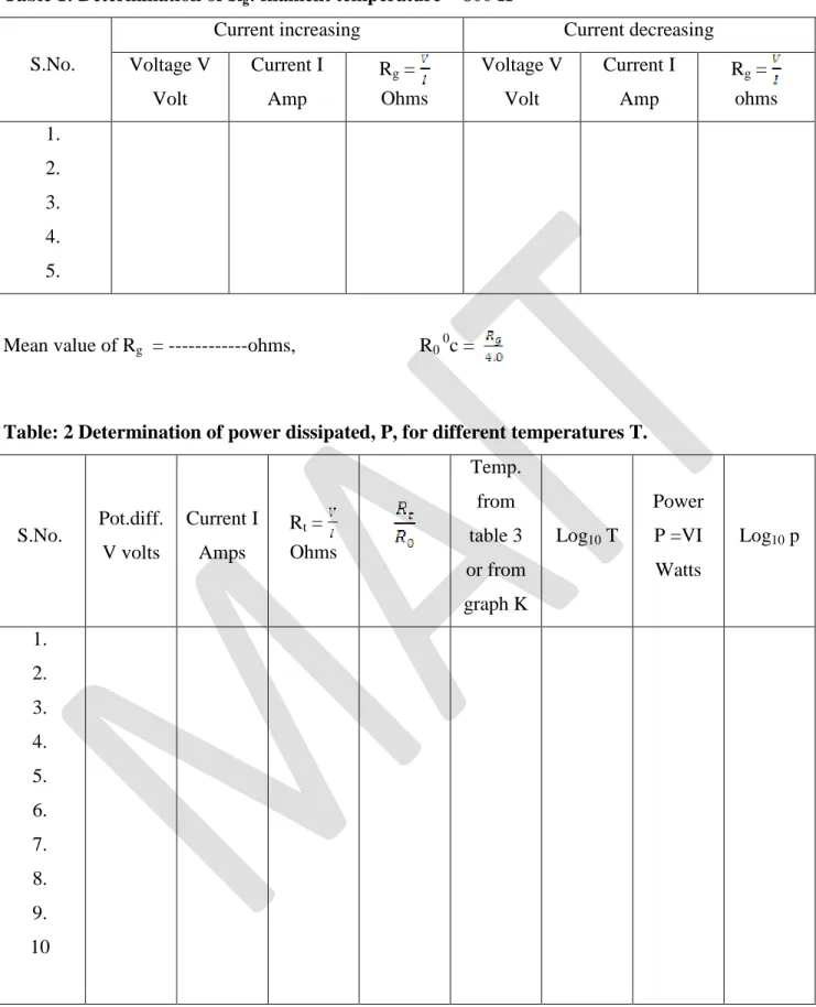
OBSERVATIONS:-
Table 1: Determination of Rg: filament temperature = 800 K
S.No.
Current increasing Current decreasing
Voltage V Volt
Current I Amp
Rg =
Ohms
Voltage V Volt
Current I Amp
Rg =
ohms 1. 2. 3. 4. 5.
Mean value of Rg = ---ohms, R0 0c =
Table: 2 Determination of power dissipated, P, for different temperatures T.
S.No. Pot.diff. V volts
Current I Amps
Rt =
Ohms Temp. from table 3 or from graph K
Log10 T
Power P =VI Watts
Log10 p
1. 2. 3. 4. 5. 6. 7. 8. 9. 10
Table:3
Graph
RESULT: - The graph of log10 p Vs log10 T is a straight line {fig}
Hence P = ATa law is verified. Because slop comes out to be 4. Hence it is a fourth power law.
Temp. in 00c Temp. in 00c
0 100 200 300 400 500 600 700
1.00 1.53 2.07 2.13 3.22 3.80 4.40 5.00
800 900 1000 1100 1200 1300 1400 1500
5.64 6.37 6.94 7.60 8.26 8.90 9.70 10.43
Experiment No.
OBJECTIVE: Calibration of a Voltmeter with a potentiometer.
APPARATUS: Potentiometer, Given voltmeter, two storage batteries, two rheostats (50,110ohm), a standard cell, galvanometer, two one-way key, one two-way key and connection wires.
PRECAUTIONS:
1. The e.m.f. of the cell used in the primary circuit should be greater than the e.m.f of standard cell.
2. All the positive terminals should be connected to the same point of the potentiometer.
3. The calibration should be checked after few readings.
4. Jockey should not be moved on the potentiometer wire
5. Voltmeter should be connected in parallel.
FORMULA USED:
The error in voltmeter reading is given by V'- V =
– V
V' =
= kl
2Where V= potentiometer difference between two points read by voltmeter
V'= potentiometer difference between the same two points read by potentiometer E= E.M.F. of the standard cell.
l1 = length of the potentiometer wire corresponding to E.M.F. of standard cell.
l2 = length of the potentiometer wire corresponding to the potential difference (V') measured by
potentiometer.
k = potential gradient of the potentiometer wire
PROCEDURE:
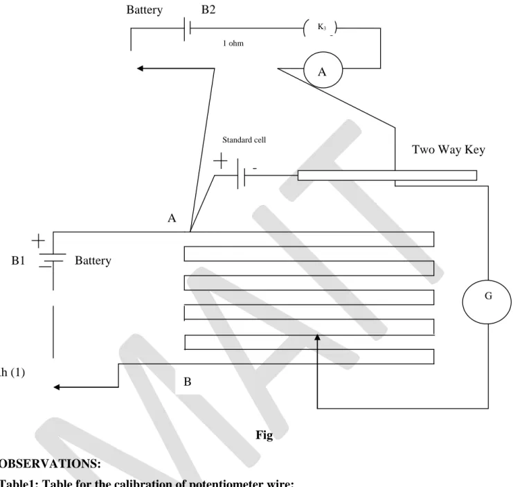
1. Make the electrical connections are show in fig (1).
2. Close K1 and insert the plug key between ‘a’ and ‘b’ terminal of key K2.Place the jockey
on the last end ‘B’ of the potentiometer wire. If the deflection is observed in the galvanometer, then the rheostat h (1) is adjusted to get zero deflection (null point). The adjustment of the rheostat is not changed throughout the experiment..
3. Record the total balancing length (l1) of the potentiometer wire. This is 1000cm for ten
wire potentiometer. The EM.F. of the standard cell (E) is recorded.
4. Now remove the plug key from the terminal between ‘a’ and ‘b’ points of key K2 and
insert it in between ‘b’ and ‘c’ terminals. Close the key K3. Again adjust the rheostat Rh(2)
[Variable point(P)] of the potential divider circuit such that the voltmeter shows a constant reading. Adjust the jockey on the potentiometer wire such that Null point in the galvanometer is obtained..
5. Note down the total length of potentiometer wire in this case (l2).
6. Now repeat the above procedure again and again and record atleast 6 -8 different values of voltmeter reading V and corresponding values of l2.
7. Now, plot a graph between the voltmeter reading (V) along the X-axis and the corresponding error in the reading (V'- V) along Y-axis. This is the required calibration curve for the given voltmeter.
Fig
OBSERVATIONS:
Table1: Table for the calibration of potentiometer wire:
e.m.f. of the standard cell (E) = 1.0286
Length of the potentiometer wire
corresponding to E.M.f. of standard cell l1 cm.
Remark
1000 E.M.F. of standard cell E =
---Volt
Potential gradient , k = E/ l1 A
B
G
V
B1
B2
Rh (2)
Rh (1)
Standard cell
Two Way Key Voltmeter
Battery
Battery
K3
K1
Table2: Table for calibration of voltmeter:
S.No.
Voltmete r reading
V volt
Balancing length of the potentiometer wire l2
V' =
(
)
= kl
2(V'- V)
No. of complete Wire
Length on sliding wire
Total l2 in
cm
1
2
3
4
5
6
Calculation:
Potential gradient , k = E/ l1 = ---volt/cm
Now V' =
(
)
or
=
kl2= --- volt
Make similar calculations for other reading
Draw a graph between the error (V’
-V) and the voltmeter reading (V) .
RESULT: The graph so obtained by plotting the error against the voltmeter reading is the calibration curve of the given voltmeter.
Standard value =
Experiment No.
OBJECTIVE: Calibration of a Ammeter with a potentiometer.
APPARATUS: Potentiometer, Given Ammeter, two storage batteries, one ohm standard resistance, two rheostats (50,110ohm), a standard cell, galvanometer, two one-way key, one two-way key and connection wires.
PRECAUTIONS:
1. The e.m.f. of the cell used in the primary circuit should be greater than the e.m.f of standard cell.
2. All the positive terminals should be connected to the same point of the potentiometer.
3. The calibration should be checked after few readings.
4. Jockey should not be moved on the potentiometer wire
5. Voltmeter should be connected in parallel.
FORMULA USED:
The error in voltmeter reading is given by I'- I =
– I
I' =
= kl
2Where I' = current reading by potentiometer I= current reading by given ammeter E= E.M.F. of the standard cell.
l1 = length of the potentiometer wire corresponding to E.M.F. of standard cell.
l2 = length of the potentiometer wire corresponding to the potential difference (I') measured by
potentiometer.
k = potential gradient of the potentiometer wire
PROCEDURE:
1. Make the electrical connections are show in fig (1).
2. Close K1 and insert the plug key between ‘a’ and ‘b’ terminal of key K2.Place the jockey
on the last end ‘B’ of the potentiometer wire. If the deflection is observed in the galvanometer, then the rheostat h (1) is adjusted to get zero deflection (null point). The adjustment of the rheostat is not changed throughout the experiment..
3. Record the total balancing length (l1) of the potentiometer wire. This is 1000cm for ten
wire potentiometer. The EM.F. of the standard cell (E) is recorded.
4. Now remove the plug key from the terminal between ‘a’ and ‘b’ points of key K2 and
insert it in between ‘b’ and ‘c’ terminals. Close the key K3. Again adjust the rheostat Rh(2)
[Variable point(P)] of the potential divider circuit such that the voltmeter shows a constant reading. Adjust the jockey on the potentiometer wire such that Null point in the galvanometer is obtained..
5. Note down the total length of potentiometer wire in this case (l2).
6. Now repeat the above procedure again and again and record atleast 6 -8 different values of ammeter reading I and corresponding values of l2.
7. Now, plot a graph between the ammeter reading (I) along the X-axis and the corresponding error in the reading (I'- I) along Y-axis. This is the required calibration curve for the given ammeter.
Fig
OBSERVATIONS:
Table1: Table for the calibration of potentiometer wire:
e.m.f. of the standard cell (E) = 1.0286
Length of the potentiometer wire
corresponding to E.M.f. of standard cell l1 cm.
Remark
1000 E.M.F. of standard cell E =
---Volt
Potential gradient , k = E/ l1 A
B
G
A
B1
B2
Rh (1)
Standard cell
Two Way Key
Battery
Battery
1 ohm
Table2: Table for calibration of voltmeter:
S.No.
Ammeter reading
I (amp)
Balancing length of the potentiometer wire l2
I' =
(
)
= kl
2(I'- I)
No. of complete Wire
Length on sliding wire
Total l2 in
cm
1
2
3
4
5
6
Calculation:
Potential gradient , k = E/ l1 = ---volt/cm
Now I' =
(
)
or
=
kl2= --- volt
Make similar calculations for other reading
Draw a graph between the error (I’
-I) and the Ammeter reading (I) .
RESULT: The graph so obtained by plotting the error against the Ammeter reading is the calibration curve of the given Ammeter.
Standard value =
Experiment No. 9A
Object: To convert a galvanometer into an ammeter of 0-3 range.
Apparatus: A galvanometer ( 30 -0 -30 ), Ammeter ( 0-3amp), a battery of different cell, two resistances boxes, a rheostat, two one way key. Screw gauge, wire and sand paper.
Precautions: 1.The cell used should have a constant e.m.f.
2. The length of the wire used as shunt should not be too small. 3. The ammeter should always be connected in series of the cell.
Theory: Let Ig be the current for maximum deflection in a galvanometer of resistance G. If this
galvanometer is to be converted into an ammeter to measure a current I, than a shunt S is appalled across its terminal such that a current Ig flows through the galvanometer and (I – Ig)
Ig = SI / S +G
Ig (S +G) =SI
IS – Ig S = Ig.G
S (I –Ig) = Ig.G
S = Ig.G / I-Ig
Where Ig =nk (n is number of division in galvanometer, K is figure of merit I is the range
of conversion.)
Procedure: 1. Determination of resistance of the galvanometer G half deflection
method.
(i) Draw the diagram showing the scheme the connections as shown in fig I and make the connection accordingly.
(ii) Take out a high resistance R say 5000 ohms from the resistance box R. Close the key K1 and adjust the value of R till the deflection is within scale and maximum in
even number.
(iii) Close the key K2 and adjust the value of the shunt resistance S so that the deflection
is reduced to half the first value. Not this deflection and the value of S.
(iv) Repeat the experiment five times for different value of deflection. To find the figure of merit:
(i) Find the e.m.f of a battery by a galvanometer. Now connect the battery, the galvanometer, the resistance box and key series as shown in fig II. Take out 5000 ohms from the resistance box and than put in the key K and adjust the value of R till you get a deflection θ = 30 divisions in the galvanometer. Note the deflection θ and R.
(ii) Take five reading by changing the deflection in galvanometer. Observation:
Resistance of galvanometer G:
S.No. Resistance
{R} Ω
Deflection {θ}
Shunt resistance {S} Ω
Deflection { } G = Ω 1. 2. 3. 4. 5.
Fig I
Figure of merit:
S.No. e.m.f (V)
Resistance {R} Ω
Deflection
{θ} K = Amp. / div.
1. 2. 3. 4. 5.
Fig II
R
G
S K2
== 2 K1
== 2
R
G K K
Calculation:
Number of division on galvanometer scale n = 30 Current for full scale deflection Ig = nk ---ampere
Range of conversion I = 3 amp
Shunt resistance S=
The value of S is usually very small and a resistance box of that range is not generally available in the laboratory. This low resistance is obtained by selecting wire of copper constantan eureka etc of a suitable diameter and length.
To find the length of wire: Find the diameter of the wire (if not given) of a copper wire and calculate the length of the wire which gives the required resistance. If
ρ = 1.78 ×10⁻⁶
ohms /cm is the specific resistance of copper and L is the length of the wire then: S =
S =
Verification:
(i) Cut a length of the wire 2 cms more than the calculated value. Connect the wire parallel to the converted galvanometer and battery, an ammeter, a key and a rheostat in series to the galvanometer as shown in fig III.
(ii)Put key K in and adjust the resistance from the resistance box so the
galvanometer shows maximum deflection. Note the reading on the galvanometer scale and corresponding reading on the ammeter. Take 4 to 5 reading by changing deflection in the galvanometer.
(iii) Plot a graph between deflection and ammeter reading.
Observations: One scale division after Conversion = amp
S.No. Galvanometer Reading Ammeter reading Difference Deflection Current in amp
1. 2. 3. 4. 5.
Result:
G A
Rh
Shunt wire
Experiment No. 9B
Object: To convert a galvanometer into a Voltmeter of 0-3 range.
Apparatus: A galvanometer ( 30 -0 -30 ), voltmeter ( 0-3v), a battery of different cell, two resistances boxes, a rheostat, two one way key. Screw gauge, wire and sand paper.
Precautions: 1.The cell used should have a constant e.m.f.
2. The Resistance should be connected in series to the galvanometer.
3. The positive of the voltmeter and battery should be connected to one terminal of the rheostat.
4. The plugs of the resistance box should be tight
Theory: Let Ig be the current for maximum deflection in a galvanometer of resistance G. If this galvanometer is to be converted into a voltmeter to measure a potential difference E, than a resistance R is placed in series with it such that the current through the galvanometer is Ig in that case:
Ig =
R =
-G
.Procedure: 1. Resistance of the galvanometer G by half deflection method.
Fig I
Draw the diagram showing the scheme the connections as shown in fig I and make the connection accordingly.
(i) Take out a high resistance R say 5000 ohms from the resistance box R. Close the key K1 and adjust the value of R till the deflection is within scale and maximum in even
number.
(ii) Close the key K2 and adjust the value of the shunt resistance S so that the deflection
is reduced to half the first value. Not this deflection and the value of S.
(iii) Repeat the experiment five times for different value of deflection.
R
G
S K2
Observation:
Resistance of galvanometer G:
S.No. Resistance
{R} Ω
Deflection {θ}
Shunt resistance {S} Ω
Deflection
{ } G =
Ω 1.
2. 3. 4. 5.
To find the figure of merit:
(i) Find the e.m.f of a battery by a voltmeter. Now connect the battery, the
galvanometer, the resistance box and key series as shown in fig II. Take out 5000 ohms from the resistance box and than put in the key K and adjust the value of R till you get a deflection θ = 30 divisions in the galvanometer. Note the deflection θ and R.
(ii) Take five reading by changing the deflection in galvanometer.
Fig II
Figure of merit:
S.No. e.m.f
(V)
Resistance {R} Ω
Deflection
{θ} K = Amp. / div.
1. 2. 3. 4. 5.
R
G K
Calculation:
Resistance of the galvanometer = ---ohms
Number of division on galvanometer scale n = 30 Current for full scale deflection Ig = nk ---ampere
Range of conversion E = 3 volt
Resistance to placed in series with the galvanometer
Verification:
(i) Draw a diagram showing the scheme of the connection as in fig III. Connect the battery of 6 volt through a key to the fixed terminal A and B of the rheostat. Connect the galvanometer through a resistance box R between the terminal A and C of the rheostat. Also connect the positive terminal of the voltmeter to a terminal and negative to C terminal of the rheostat.
(ii) Take out a resistance equal to calculated value of R of the resistance box and keeping the moveable contact near A put in the key k. Note the reading of the galvanometer and voltmeter move the variable contact and take about 4 to5 observation by changing deflection in the galvanometer.
(iii) Plot a graph between deflection and Voltmeter reading R = -G
Fig III
Observations: One scale division after Conversion = = volt S.No. Galvanometer Reading Voltmeter
reading
Difference Deflection in volt
1. 2. 3. 4. 5.
Result:
V
G R
Rheostat
Experiment 10
Object: To determine the energy band gap of semiconductor material by four probe method.
Apparatus: Probes arrangement, Sample (Ge crystal), Oven, Four probe set up, Thermometer.
Precautions:
1. The surface on which the probe rest should be uniform.
2. Do not exceed the temperature of the oven above 1800 for safe side. 3. Semiconductor crystal with four probes is installed in the oven very carefully otherwise the crystal may damage because it is brittle. 4. Current should remain constant throughout the experiment.
5. Minimum pressure is exerted for obtaining proper electrical contacts to the chip.
Formula used: The resistivity of the semiconductor crystal given by ρ =
Where ρ0 =
G (W/S) is the correction factor and this obtained from table for the appropriate value of (W/S) W is the thickness of the crystal S is the distance between probe V and I are the voltage and current across and through the crystal chip. The energy band gap Eg of semiconductor crystal is given by
Eg 2K × eV
Where K is Boltzmann constant = 8.6 ×10⁻⁵ eV / deg and T is temperature in Kelvin
Theory: The Four Probe Method is one of the standard and most widely used methods for the measurement of resistivity of semiconductors. The experimental arrangement is illustrated. In its useful form, the four probes are collinear. The error due to contact resistance, which is especially serious in the electrical measurement on semiconductors, is avoided by the use of two extra contacts (probes) between the current contacts. In this arrangement the contact resistance may all be high compare to the sample resistance, but as long as the resistance of the sample and contact resistances are small compared with the effective resistance of the voltage measuring device (potentiometer, electrometer or electronic voltmeter),the measured value will remain unaffected. Because of pressure contacts, the arrangement is also especially useful for quick measurement on different samples or sampling different parts of the same sample.
Description of the experimental setup
1.ProbesArrangement
It has four individually spring loaded probes. The probes are collinear and equally spaced. The probes are mounted in a teflon bush, which ensure a good electrical insulation between the probes. A teflon spacer near the tips is also provided to keep the probes at equal distance. The whole –arrangement is mounted on a suitable stand and leads are provided for the voltage measurement.
2.Sample
Germanium crystal in the form of a chip
3.Oven
It is a small oven for the variation of temperature of the crystal from the room temperature to about 200°C (max.)
4.FourProbeSet-up,
The set-up consists of three units in the same cabinet.
Procedure:
1. Connect the outer pair of probes to current source through current terminal and the inner pairs to the probe voltage terminal.
2. Place the four probe arrangement in the oven and fix the thermometer in the oven through the hole.
3. Switch on the four probe set up and adjust the current to a desired value (say 8 mA) .Change the knob on the voltage side.
4. Connect the oven power supply. Rate of heating may be selected with the help of a switch low or high.
5. Switch on the power to the oven and heating will start.
6. Measure the voltage by putting the digital panel meter in voltage measuring mode and temperature (
0
c)in thermometer.
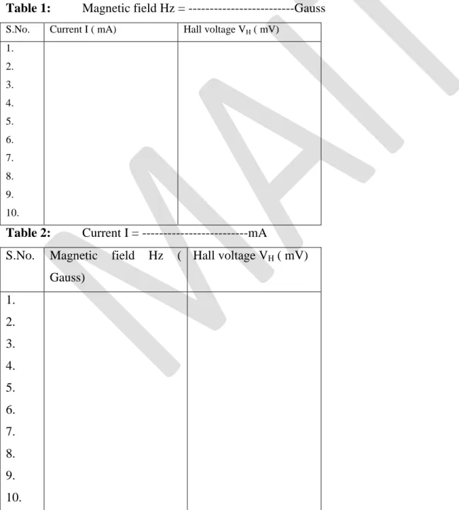
Observations Table:
Distance between probes (S) = 0.200 cm Thickness of the crystal (W) = 0.050 cm Constant current (I) = 8.00mA
S.No Temperature (00)
Voltage (volts)
Temperature (T in K)
ρ0=
(ohm cm)
ρ =
(ohm cm)
×103
log 10ρ
1. 2. 3. 4. 5. 6. 7. 8. 9. 10. 11. 12. 13. 14. 15. 16. 17. 20 30 40 50 60 70 80 90 100 110 120 130 140 150 160 170 180
Table: G (W/S) function corresponding to (W/S) geometry of the crystal
S.No W/S G (W/S)
1. 2. 3. 4. 5. 6. 7. 8. 9. 10. 11.
0.100 0.141 0.200 0.33 0.500 1.000 1.414 2.000 3.333 5.000 10.000
13.863 9.704 6.931 4.159 2.780 1.504 1.223 1.094 1.0228 1.0070 1.00045
Calculation:
Find ρ corresponding to temperature in K using ρ =
Where ρ0 = = ---ohm cm
For different ‘V’ calculate ρ0 and hence ρ in ohm cm
Find {W/S} and then corresponding to this value choose the value of function
Graph Now plot a graph for logρ versus ×10-3 as shown in
fig
Slop of the curve is
Energy band gap Eg = 2K ×
= 2K × 2.303 × × 1000 = 4.606 × 8.6 ×10-5× × 1000 ` = 0.396 × ev
Result: 1. Resistivity of semiconductor crystal at different temperature are shown in the graph of log 10ρ versus ×10-3
2. Energy band gap o semiconductor crystal Eg = ---eV
Standard Eg : Ge = 0.72 eV Si = 1.1 eV