Thesis

(1)

Determinants of exposure to household air pollution in rural Malawi

By

Sangeetha Kumar

Senior Honors Thesis

Curriculum for Environment and Ecology University of North Carolina at Chapel Hill

(2)

Abstract

The very high exposure of people to airborne combustion products in developing

nations who use solid fuels (mainly wood) as the only source of fuel for cooking, often in

inefficient stoves and with poor ventilation is an important public health and

environmental issue. A research study done by UNC’s FUEL (Forest Use, Energy, and

Livelihoods) Lab collected data on determinants of exposure to household air pollution in

rural Malawi. The field study collected carbon monoxide (CO) and particulate matter

(PM2.5) for a period of 24 hours in each of the 108 households in the study. Additionally,

they collected both personal (the primary cooks of the household wore the monitors) and

area (placed in the primary cooking area) concentration measurements along with

completing an in-depth questionnaire with the household owners.

The goal of the study was to do a multivariate regression analysis of household

pollutant levels to see how different factors – the type of fuel, fuel quality, stove design,

ventilation conditions, etc. – influence indoor air pollutant exposures. The study found

that the interaction of ventilation, moisture content, stove type, income quintile, and household size in a multivariate regression model best explains the variance of household air pollutant concentrations. The identification of these determinants allows for further studies on targeted interventions that reduce pollutant concentrations and adverse health

(3)

Acknowledgements

(4)

List of Tables

Table 1: Descriptive statistics for dependent variables

Table 2: Descriptive statistics for categorical independent variables

Table 3: Comparison of means test for categorical independent variables

Table 4: Descriptive statistics for continuous independent variables

Table 5: Multivariate regression analysis using stove type, fuel type, fuel quantity, ventilation, and moisture content as inputs.

Table 6: Multivariate regression analysis using stove type, fuel type, fuel quantity, household size, ventilation, and moisture content as inputs

Table 7: Multivariate regression analysis using stove type, fuel type, fuel quantity, household size, ventilation, income quintiles, and moisture content as inputs

(6)

List of Figures

Figure 1: Graphical representation of the variability of PM2.5 concentrations

Figure 2: Graphical representation of the variability of CO concentrations

Figure 3: Graphical representation of the variability of BC concentrations

Figure 4: Descriptive statistics for dependent variables (histogram distributions)

Figure 5: Histogram distributions for continuous independent variables

Figure 6. Dependence of particle concentrations on moisture content

Figure 7: Dependence of particle concentrations on fuel quantity

Figure 8: Dependence of particle concentrations on household size

(7)

Introduction

About half the world’s population relies on biomass fuels as a means to meet their

domestic energy requirements particularly for cooking (Barnes, 2014). The dependence

on biomass fuel is the greatest in rural areas; specifically in African countries, it

constitutes 70% of energy needs (Rumchev et. al, 2007). It is difficult to burn solid fuels in simple combustion devices without a sizable emission of pollutants. This leads to a

substantial fraction of the fuel carbon being converted to products of incomplete

combustion rather than compounds such as carbon dioxide that result from complete

combustion (Zhang et al., 2000).

Products of incomplete combustion include, but are not limited to carbon

monoxide (CO) and particulate matter (PM). The PM typically generated from fuel

combustion is fine or ultrafine in size, but larger particles may result from ash and solid

fuel fragments (Zhang et al., 2000). The size of the particulate matter is a determinant for

assessing health impacts. Typically, a fine or ultrafine particle can easily travel within the

respiratory tract leading to detrimental health effects. It is estimated that 4 million deaths

occur annually due to indoor air pollution, or 2.7% of the global burden of disease

(especially due to respiratory illness) (Lim et al., 2010). Global burden of disease refers

to the lost healthy life years due to premature death and illness (Zhang et al., 2003). The Global Burden of Disease Project estimates that household air pollution (HAP) is

(8)

who spend the predominant amount of time near the kitchen area.

The goal of the study is quantitatively assess the determinant exposure response

relationship. To do this, certain determinants of exposure—including biophysical and

behavioral causes—are reviewed for their effects on particle concentrations in up to date

literature. It is particularly important to identify determinants of household air pollution

in order to find effective mitigation and intervention strategies to reduced indoor air

pollution. Not only is indoor air quality with regards to cookstove emissions an important

health outcome, but it has implications on climate as well. Cookstove emissions

contribute to the ever-increasing greenhouse gases and black carbon in the atmosphere

(Rosa et. al, 2014). Additionally, using biofuels as a primary energy source may lead to deforestation, another contributor to greenhouse gas emissions.

Fuel type

Fuel type was found to be most important determinant of pollution in both Mehta

et al. (2002) and Balakrishnan et al. (2002). In a 1996 study, it was shown that biomass

(9)

With respect to just biomass fuels—wood crop residue, and dung—approximately two fifths of the world’s households rely on biomass as their principal fuel type (Smith,

1994). Studies show that approximately 80% of the world’s population exposure to

particulate matter indoors is due to the emissions from biomass fuels—wood, crop

residue, and dung (Chaudhuri et. al 2003). The use of biomass as the primary fuel source

results in using a lower efficiency stove. In particular, wood burning stoves were found

on average contribute 50 times more pollution during cooking in comparison to a gas

stove (Smith, 1994).

Moisture content

Moisture content refers to the measure of the amount of water in a fuel, and is expressed as percent of the dry weight of the fuel. For a fire to burn more intensely, the moisture content of the fuel must be lower than the moisture content of the extinction of fire (Hoffa et al., 1999). The drier fuels burn more intensely than the wet because of less latent heat transfer; subsequently, the lower intensity fires of wet fuels produce more products of incomplete combustion including CO and PM2.5 (Hoffa et al., 1999).

Moisture content is also considered to be undesirable because it results in lower thermal emissions and has also been linked to higher emissions of aerosols or VOCs (McDonald et al. 2000). When using improved stoves that are capable of producing less CO and PM, the moisture content of the fuel used can lead to lower performance (Adler, 2010).

Stove Design

(10)

introductions into communities. In order for each stove type to be evaluated equally across the board on the same parameters, the Global Alliance for Clean Cookstoves developed an International Working Agreement (IWA) in 2012 on guidance for rating cookstoves. Cookstoves are rated based on four performance indicators: fuel use, total emissions, indoor emissions, and safety. To highlight progress in furthering improvement in cookstove design, each performance standard has multiple tiers of performance (valued from 0 to 4). Each stove type has up to four ratings for Tiers of Performance (one for performance indicator).

Many areas of the developing world are reliant on simple open-fire cookstoves

that not only increase pollutant concentrations but cause adverse health outcomes for

women and children. Burning biomass fuels in low efficiency stoves such as traditional,

open-fire three stone stoves can emit smoke containing significant quantities of pollutants

(Balakrishnan et al., 2004). Open fires and old-fashioned cookstoves emit 90% CO, the other 10% being a mix of VOCs, PAHs (polyaromatic hydrocarbons), metals, and

variously sized particular matter (Adler, 2010). There’s a strong need to improve stove

efficiency as a method to increase combustion efficiency. The transition to more clean and efficient energy systems for cooking are also based on per capita incomes—the higher the more likely the switch (Balakrishnan et al., 2004). On the other hand, appliances that burn fossil fuels have higher combustion efficiencies and therefore generate insignificant amounts of CO (Zhang et al., 2003). Stoves that are not vented— have a flue or hood—do not take pollutants out of the living area (Smith et al. 2002). A

Randomized Exposure Study of Pollution Indoors and Respiratory Effects (RESPIRE) in

(11)

90% (Smith). Intervention studies for improved cook stoves found reductions in

concentrations of CO and PM for kitchen level and personal concentrations (Bruce et al.,

2004, Albalak et al.,2001, Cynthia et al.,2008, Rosa et. al, 2014).

Ventilation

Kitchen ventilation (based on air exchange rates) and cooking location have

profound impact on the level of household air pollutant concentrations (Rosa et al., 2014)

(Ruth et al.,2013). A test kitchen study with biomass stoves found that increasing air

exchange rates by opening windows and doors reduced PM2.5 1-hour concentrations by

93-98% compared to the closed kitchen and CO concentrations by 83-95% less (Grabow

et al., 2013). Additionally, studies characterize ventilation as a function of the number of

doors and windows open as in an indication of the air exchange rate. A study done by

Rumchev et al. found a significant relationship between window area and concentration

of CO and PM2.5. The increase in window area was associated with reduction in the

concentration of PM2.5 and CO. Additionally, for PM2.5, the increase in number of

windows saw a reduction in PM2.5 concentrations as well. It can be concluded from this

study that using biofuels indoors in a poorly ventilated environment can cause an increase

in air pollutants.

A study (Albaklak et al., 1999) done in Bolivia measured PM10 concentrations in

two different villages in Bolivia—one characterized by indoor cooking the other with

outdoor cooking. The analysis of their pollutant concentrations of PM10 found that there

were significant effects of indoor vs. outdoor cooking on the pollutant levels.

(12)

µg/m3 in comparison to outdoor kitchen environments 280 µg/m3. On the other hand,

when smoke is released outdoors indoor levels can become high where a large population

of households use solid fuels (Zhang et al.,2000). This is due to the re-entry of pollution

back into households and is typically associated with cold winter weather with poor

atmospheric dispersion (Zhang et al.,2000). Outdoor cooking “in the intervention was associated with a median reduction of 73% when compared to control households (p<0.001), 57% reduction when compared to indoor-cooking intervention homes (p=0.02). (Rosa et. al, 2014)

Methodology

Study Setting

The Forest Use, Energy and Livelihoods Lab (FUEL) collected data on determinants of exposure to household air pollution in Malawi as a part of the Malawi Forest and Livelihoods Survey (MFLS) from October to November of 2013. The sample of population was drawn

(13)

Malawi with high forest reliance and active forest co-management agreements. The districts are marked in red on the map entitled MFLS Survey Sites.

The villages of interest within the Machinga District are located adjacent to the

Liwonde Forest Reserve, which is a significant source of fuelwood and charcoal. This

area has good market access due to its proximity to three of Malawi’s 15 largest urban

centers (Balaka, Liwonde, and Zomba). The main agricultural crops of the region are

maize and paddy rice. Households keep chickens and other small animals, but overall

there is limited investment in livestock.

In comparison to the Machinga District, Kasungu has a lower population density. It is located approximately 300 kilometers north of Malawi’s capital—Lilongwe;

additionally, the villages of interest within the district are adjacent to the Chimaliro Forest Reserve, which has a significant source of fuelwood. Access to markets is limited in the region, but there are major markets due to international trade with Zambia. The main agricultural crops of the region are maize and tobacco; additionally, in the wetland areas (dambos) a variety of vegetables are grown. Unlike Machinga, Kasungu households invest in livestock including cattle and goats.

(14)

partake in the study by being given a chitenge (a form of cloth). Each house chosen in the study responded to questions to describe their household demographics, assets,

agricultural production, expenditures, access to forest resources, etc. The primary cooks also answered questions about household food consumption, kitchen design and

ventilation, fuel use, cooking technology choices, indicators of health status, etc. The results from the questionnaires, in particular of relation to cooking, were used for this analysis.

Indoor air pollution measurements

The protocol of the study required collection of carbon monoxide (CO) and

particulate matter (PM2.5) for a period of 24 hours. The data collection was done in two

parts —area exposure and personal exposure monitoring. The instruments for both the

CO and PM2.5 monitoring were mounted at a height of 1.5 meters on a tripod positioned 1

meter away from the stove. For the personal exposure monitoring, the CO monitor and

the PM2.5 monitor (including the pump and the filter) were placed in a side messenger

bag or backpack for the women to hold.

Carbon monoxide was measured using a Lascar CO Data Logger (model

EL-USB-CO) (Lascar Electronics, Salisbury, UK) at a sample rate of once a minute for a

total of 24 hours. These monitors are accurate to ±6 ppm, with a range of 0 to 1000 ppm.

To ensure accuracy, certain households were chosen to detect variance in measurements

(15)

Particulate matter (PM2.5) was collected on a 2µm polytetrafluoroethylene (PTFE)

filter over the course of a 24-hour period. Each personal and area PM2.5 filter was

attached to a SKC AirChek XR5000 pump connected to a SKC Personal Environmental

Monitor for PM2.5 sampling (SKC, Inc., Eighty Four, PA, USA) that was calibrated to a

flow rate of 2 (±0.5%) (L/min). The area pump was turned on once ever 6 minutes (i.e. 1

minute on, 5 minutes off, 240 cycles); whereas, the personal pump was continuously run.

These filters were weighed prior to use, and weighed subsequently after the 24-hour

study period in the household using a MX5 Microbalance (Mettler-Toledo, Inc.,

Columbus, Ohio) after being equilibrated for at least 24 hours in a Secador 1.0 Dessicator

Cabinet (Bel-Art Products, Inc., Wayne, New Jersey) at 33% relative humidity.

Data Analysis

Processing emissions

The carbon monoxide (CO) measurements were averaged across the collected data points over the 24 hr. period to get the 24 hr.-period CO personal and area average concentrations measured in ppm (parts per million). Each of the carbon monoxide monitors used were corrected for their experimental correction factor—these calibration correction factors were found experimentally in the lab setting prior to using the

monitors. See Appendix B for Carbon Monoxide correction factors.

Particulate Matter (PM2.5) measurements were calculated using the net mass

(16)

masses. To convert the net mass to a particulate matter concentration (µg /m3

), the following equation was used:

!"## !" !"#$%& × !"""

!"#$ !"#$%&'( × !"#$ !"#$

!"""

(1)

The pump duration (min) is the length of time that the pump was turned on, typically 240 minutes for the area pumps and 1440 min for the personal pumps. The pump rate (L/min) is the rate at which is air flowed into the filter, typically around 2 L/min for both the area and personal pumps. The PM2.5 data proved to be problematic

because there were negative concentrations and negative net gain in mass. Negative concentrations follow from negative masses as evident from equation (1). The second

issue may be attributed to an error in weighing the filters. Additionally, personal PM2.5 concentrations were larger than respective area PM2.5 concentrations for certain

households. To attempt to understand these varying values, the amount of black carbon (BC) in each filter was estimated using a Nexleaf algorithm, which takes a photo of the filter as an input and outputs the amount of black carbon that was in the air. The

concentrations of BC (µg /m3_{), were calculated the same ways at the PM2.5.}

Baseline characteristics

Initial data analysis was done to understand the variability of the particle

concentrations of interest—area and personal PM2.5 concentrations, area and personal CO

concentrations, and area and personal BC concentrations. A t-test was done to identify

the significance of the difference of means between area and personal concentrations.

Additionally, initial plotting was completed to show the relationship between area and

(17)

Using the cook and household survey data as well as relevant literature, certain

parameters were chosen as a test to explain household air pollution exposures. These

parameters include moisture content, fuel quantity, fuel type, stove type, income

quintiles, household size, ventilation, and cooking experience. Moisture content (%) was

obtained using an Ohaus MB23 Moisture Analyzer (Parsippany, NJ). The fuel quantity

was calculated as the the sum of difference in the amount of fuel at the beginning and end

of the 24 hr study period and the amount of fuel added in the study period. Fuel type is a

categorical variable taking the value of 0 for low quality fuel wood, and 1 for high quality

fuel wood. Stove type is a categorical variable taking the value of 0 for a 3 stone

(traditional stove) and 1 for a non-traditional stove. Income quintile is a categorical

variable taking the value of 0 for the lowest income bracket and 5 for the highest income

bracket of the subset of households. Household size refers to the number of adult

equivalents in each household—coded as 1 for each adult and 0.5 for each child.

Ventilation is a categorical variable that takes the value of 0 for poorly ventilated

kitchens and 1 for well ventilated kitchens—typically those with more windows and

doors or those outdoors. Cooking experience is a continuous variable that refers to the

number of years of cooking experience the primary cook has had in any household.

T-tests and regressions were performed to see the significance of the relationship between

each pollutant concentration and parameter.

Multivariable Regression Analysis

(18)

dependent variables of interest include the personal and area particulate matter

concentrations, the personal and area carbon monoxide concentrations, and the personal and area black carbon concentrations. The independent variables – the determinants for household exposure—are the aforementioned parameters found from the household and cooking data.

𝑌

_!

=

𝛽

_!

𝑋

_!_!

+

𝛽

_!

𝑋

_!!

+

⋯

+

𝛽

_!

𝑋

_!"

+

𝜀

_!

A multivariable regression model of this form is as shown above where

𝑌

_! is the

dependent variable of interest, and

𝑋

_!" are the independent variables with coefficients

(19)

Results

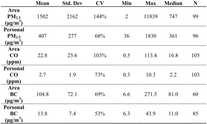
Table 1: Descriptive statistics for dependent variables

Mean Std. Dev CV Min Max Median N Area

PM2.5

(µg/m3)

1502 2162 144% 2 11839 747 99

Personal PM2.5

(µg/m3)

407 277 68% 36 1830 361 96

Area CO (ppm)

22.8 23.6 103% 0.5 113.4 16.8 105

Personal CO (ppm)

2.7 1.9 73% 0.3 10.3 2.2 103

Area BC (µg/m3)

104.8 72.1 69% 6.6 271.5 81.0 60

Personal BC (µg/m3)

13.8 7.4 53% 6.3 43.9 11.0 85

Table 1 shows the mean, standard deviation, the coefficient of variance,

minimum, maximum, medium and sample size of the set of air pollutant concentrations.

The sample size (N) of Table 1, is lower than the number of households in the subset

(108) due to the removal of outliers. Large outliers within the subsets of personal and

area concentrations PM2.5 were removed. Low-concentration filters of BC have biased

estimates of BC mass because the study used Teflon filters instead of Quartz (which is

the type of filter the Nexleaf algorithm is based on). Additionally, these filters drove the

average ratio of BC to PM2.5 ratios up. Subsequently, data was omitted when the BC mass

was less than 0.0176 mg—or 150% of the blank filters average mass (0.0117 mg).

(20)

area and personal exposures. To view descriptive statistics for the original full data set,

see Appendix D.

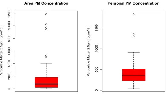
Figure 1: Graphical representation of the variability of PM2.5 concentrations

0

2000

4000

6000

8000

10000

12000

Area PM Concentration

Pa

rt

icu

la

te

Ma

tte

r

2.

5µ

m

(µ

g/

m^

3)

0

500

1000

1500

Personal PM Concentration

Pa

rt

icu

la

te

Ma

tte

r

2.

5µ

m

(µ

g/

m^

(21)

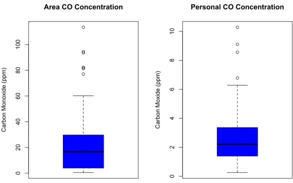
Figure 2: Graphical representation of the variability of CO concentrations

Figure 3: Graphical representation of the variability of BC concentrations

0

20

40

60

80

100

Area CO Concentration

C

arb

on

Mo

no

xi

de

(p

pm)

0

2

4

6

8

10

Personal CO Concentration

C

arb

on

Mo

xi

de

(p

pm)

0

50

100

150

200

250

Area BC Concentration

Bl

ack

C

arb

on

(µ

g/

m^

3)

10

20

30

40

Personal BC Concentration

Bl

ack

C

arb

on

(µ

g/

m^

(22)

Figures 2, 3, and 4 above show boxplots of the area PM2.5 concentration, area CO

concentration, area BC concentration, personal PM2.5 concentration, personal CO

concentration, and personal BC concentration. These plots depict the spread of the distribution of each concentration subset by dividing each data point into its respective quartiles. The “whiskers” of each plot represent the 95% CI and the thick dark line represents the mean of the concentrations. Comparing the difference in means of the area and personal concentrations of PM2.5, CO, BC shows that the difference is very

statistically significant—the 95% confidence intervals do not overlap. Relative to the WHO standards for PM2.5 exposure guidelines—mean

concentration of 24-hour period should not exceed 25 µg/m3—the 95% CI of both the personal and area concentrations lie above this threshold. Similarly, the EPA National

Ambient Air Quality Standards for PM2.5 exposure guidelines—mean concentration of

24-hour period should not exceed 35 µg/m3_{—our data lies above this as well. Relative to the} WHO standards for CO exposure guidelines—mean concentration of 24 hour period

should not exceed 7 mg/m3 or 6.11 ppm—the 95% CI of personal and area concentrations of CO contains this threshold. However, the personal concentrations are closer in value to

the mean WHO threshold.

- Personal PM and area PM relationship is statistically significant at the p(<0.05) level. R2

value was 0.060.

- Area CO and personal Co are statistically significant at the (p<0.001) level R2

value was 0.109.

- Area BC and personal BC are statistically significant at the (p<0.05) level R2

(23)

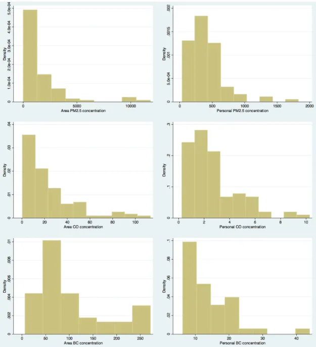
Figure 4: Descriptive statistics for dependent variables (histogram distributions)

Figure 3 above shows the distributions of area PM2.5 concentration, personal PM2.5

(24)

are used for the multivariate regression analysis. A table of descriptive statistics for the log-transformed values can be seen in the Appendix.

Profile of study populations

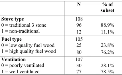
Table 2: Descriptive statistics for categorical independent variables

N % of

subset

Stove type 108

0 = traditional 3 stone 96 88.9%

1 = non-traditional ₁₂ _11.1%

Fuel type 105

0 = low quality fuel wood 25 23.8%

1 = high quality fuel wood ₈₀ _76.2%

Ventilation 107

0 = poorly ventilated 30 28.1%

1 = well ventilated 77 78.5%

Table 2 describes the sample size N and percentage of subset for the categorical

independent variables for the multivariate regression model including stove type, fuel

type, and ventilation. The subset of households in the study, had 88.9% traditional

3-stone stoves, 76.2% use of high quality fuel, and 78.5% had well ventilated kitchen.

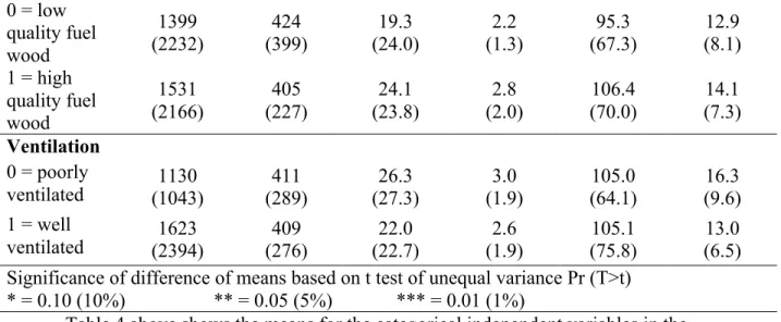
Table 3: Comparison of means test for categorical independent variables

Area

PM2.5

Conc. (µg/m3)

Area CO Conc. (ppm)

Personal CO Conc. (ppm)

Area BC Conc. (µg/m3)

Personal BC Conc. (µg/m3)

Stove type 0 = 3 stone

traditional ₍₂₂₇₂₎1544 ₍₂₇₆₎396 _(22.7)21.3 _(1.8)2.6 _(70.8)100.4 _(7.5)13.7 1 =

(25)

0 = low quality fuel wood

1399

(2232) (399) 424 (24.0) 19.3 (1.3) 2.2 (67.3) 95.3 (8.1) 12.9 1 = high

quality fuel wood

1531 (2166)

405 (227)

24.1 (23.8)

2.8 (2.0)

106.4 (70.0)

14.1 (7.3) Ventilation

0 = poorly

ventilated ₍₁₀₄₃₎1130 ₍₂₈₉₎411 _(27.3)26.3 _(1.9)3.0 _(64.1)105.0 _(9.6)16.3 1 = well

ventilated ₍₂₃₉₄₎1623 ₍₂₇₆₎409 _(22.7)22.0 _(1.9)2.6 _(75.8)105.1 _(6.5)13.0 Significance of difference of means based on t test of unequal variance Pr (T>t)

* = 0.10 (10%) ** = 0.05 (5%) *** = 0.01 (1%)

Table 4 above shows the means for the categorical independent variables in the

multivariate regression model including stove type, fuel type, and ventilation. In addition,

the significance for the difference of means (assuming unequal variances) of each subset

is noted in the categorical variable heading. There was no significant difference between

the mean values of the categorical variable, meaning that the 95% CI of each coded value

of the categorical variable (i.e. 0 or 1) significantly overlapped.

Table 4: Descriptive statistics for continuous independent variables

Mean Std. Dev CV Min Max Median N Moisture

content (%) 11.4 6.4 56% 1.4 43.4 9.9 106 Fuel

quantity

(kgs) 17.5 19.8 113% 0.5 159.9 12.6 106 Household

Size (# adult equivalents)

4.5 2.0 44% 1 11 4 107

Fuel quantity by

household size (kgs/ adult equiv)

4.5 7.9 176% 0.2 80.0 3.1 105

Cooking experience

(26)

Table 4 above shows the mean, standard deviation, the coefficient of variance,

minimum, maximum, medium and sample size of each continuous independent variable

of interest—moisture content, fuel quantity, household size, fuel quantity by household

size, and cooking experience.

(27)

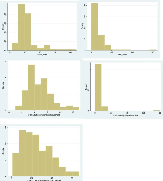
The figures above show thedistributions of the continuous independent

variables (from left to right, top to bottom) moisture content (%), fuel quantity (kgs), household size (# adult equivalents), fuel quantity by household size, and cooking experience (years). Looking at these plots, each particle concentration subset follows a log normal distribution. A log transformation of each independent variable will closely follow a normal distribution. Therefore, when completing the multi-regression analysis, the log-transformed values will be used.

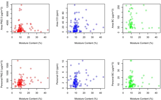
Figure 6. Dependence of particle concentrations on moisture content

The figures above show plots of the area PM2.5 concentration, area CO

concentration, and personal BC concentration as a function of moisture content. Basic

0 10 20 30 40

0

4000

8000

12000

Moisture Content (%)

Are a PM2 .5 (µ g/ m^ 3)

0 10 20 30 40

0

20

40

60

80

Are a C O (p pm)

0 10 20 30 40

0

50

150

250

Are a BC (µ g/ m^ 3)

0 10 20 30 40

0

500

1000

1500

Pe rso na l PM2 .5 (µ g/ m^ 3)

0 10 20 30 40

0 2 4 6 8 10

Pe rso na l C O (p pm)

0 10 20 30 40

10

20

30

40

(28)

correlation testing found a statistically significant relationship between moisture content and personal PM3.5 concentrations as well as with personal CO concentrations at the

p(<0.05) level.

Figure 7: Dependence of particle concentrations on fuel quantity

concentration, and personal BC concentration as a function of fuel quantity. Basic correlation testing between exposures and fuel quantity found no significant relationship for any of the six measured exposures.

0 50 100 150

0

4000

8000

12000

Fuel Quantity (kgs)

Are a PM2 .5 (µ g/ m^ 3)

0 50 100 150

0

20

40

60

80

Fuel Quantity (kgs)

Are a C O (p pm)

0 50 100 150

0

50

150

250

Fuel Quantity (kgs)

0 50 100 150

0

500

1000

1500

Fuel Quantity (kgs)

0 50 100 150

0 2 4 6 8 10

Fuel Quantity (kgs)

0 50 100 150

10

20

30

40

Fuel Quantity (kgs)

(29)

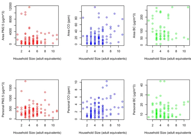
Figure 8: Dependence of particle concentrations on household size

concentration, and personal BC concentration as a function of household size. Basic correlation testing found a statistically significant relationship between household size and area and personal CO concentrations at the p(<0.01) level.

2 4 6 8 10

0

4000

8000

12000

Household Size (adult equivalents)

Are a PM2 .5 (µ g/ m^ 3)

2 4 6 8 10

0

20

40

60

80

Are a C O (p pm)

2 4 6 8 10

0

50

100

200

2 4 6 8 10

0

500

1000

1500

2 4 6 8 10

0 2 4 6 8 10

2 4 6 8 10

10

20

30

40

(30)

Figure 9 Dependence of particle concentrations on moisture cooking experience

concentration, and personal BC concentration as a function of cooking experience. Basic correlation testing found a statistically significant relationship between cooking

experience size and personal PM2.5 concentrations at the p(<0.05) level.

Regression Analysis

Table 5: Multivariate regression analysis using stove type, fuel type, fuel quantity, ventilation, and moisture content as inputs. The table below shows the coefficient, standard error, and the level of significance for each species’ multivariate regression models.

Area

PM2.5

Conc. (µg/m3)

Area CO Conc. (ppm) Personal CO Conc. (ppm) Area BC Conc. (µg/m3)

0 10 20 30 40 50 60

0

2000

6000

10000

Cooking Experience (years)

Are a PM2 .5 (µ g/ m^ 3)

0 10 20 30 40 50 60

0 20 40 60 80 100

Are a C O (p pm)

0 10 20 30 40 50 60

0 50 100 150 200 250

0 10 20 30 40 50 60

0

500

1000

1500

0 10 20 30 40 50 60

0 2 4 6 8 10

0 10 20 30 40 50 60

10

20

30

40

(31)

Stove type (1= non-traditional)

0.372

(0.48) (0.21) 0.229 0.823 (0.42) * (0.24) 0.220 (0.34) 0.442 (0.19) 0.008 Moisture

content (%) _(0.32)0.132 0.301 _(0.14)** _(0.29)0.374 _(0.16)0.218 _(0.20)0.031 _(0.13)0.070 Fuel type

(1 = high quality fuel wood) 0.117 (0.37) 0.026 (0.17) 0.236 (0.34) 0.222 (0.19) 0.189 (0.24) 0.089 (0.12) Fuel quantity (kg) -0.025 (0.22) -0.041 (0.10) -0.057 (0.20) -0.002 (0.11) 0.035 (0.13) 0.087 (0.08) Ventilation (1= well ventilated) -0.136 (0.37) -0.015 (0.16) -0.213 (0.34) -0.223 (0.19) -0.071 (0.23)

-0.251 * (0.13) Error

Constant _(0.96)6.189 _(0.43)5.193 _(0.88)1.572 _(0.49)0.222 _(0.62)4.154 _(0.38)2.252 R2 value 0.0134 0.0708 0.0749 0.0647 0.0573 0.0766 Notation for significance based on p-values of the regression

* = 0.10 (10%) ** = 0.05 (5%) *** = 0.01 (1%)

Looking at the first regression in Table 5, using stove type, fuel most used, fuel quantity, ventilation, and moisture content as inputs, the model demonstrates that use of a non-traditional stove has a positive and weakly significant effect on area CO exposures.

Moisture content has a positive and significant effect on personal PM2.5 exposures;

therefore, as moisture content increases so does the exposure concentration. Improved

ventilation has a negative and weakly significant effect on personal BC exposures.

Table 6: Multivariate regression analysis using stove type, fuel type, fuel quantity, household size, ventilation, and moisture content as inputs. The table below shows the coefficient, standard error, and the level of significance for each species’ multivariate regression models.

Area

PM2.5

Conc. (µg/m3)

Stove type

(32)

Moisture

content (%) _(0.32)0.119 0.319** _(0.15) _(0.29)0.323 _(0.16)0.165 _(0.20)0.033 _(0.13)0.086 Fuel type

(1 = high quality fuel wood) 0.099 (0.38) 0.051 (0.17) 0.167 (0.35) 0.152 (0.19) 0.229 (0.24) 0.103 (0.13) Fuel quantity (kg) -0.037 (0.22) -0.023 (0.10) -0.107 (0.20) -0.054 (0.11) 0.057 (0.13) 0.092 (0.079) Ventilation (1= well ventilated) -0.136 (0.37) -0.015 (0.16) -0.209 (0.34) -0.218 (0.19) -0.021 (0.23) -0.246* (0.13) Household

size (# adult equivalents) 0.083 (0.36) -0.117 (0.16) 0.353 (0.33) 0.368** (0.18) -0.289 (0.23) -0.062 (0.13) Error

* = 0.10 (10%) ** = 0.05 (5%) *** = 0.01 (1%)

Table 6’s model looked at the influence adding household size to the original list

of determinants. This model finds that household size has a positive and significant effect

and personal CO exposures, meaning that the increase in the number of adult equivalents

in a household corresponds to an increase in personal CO exposures. A similar model

was run considering fuel quantity as a function of household size, but found no

statistically significant effect (See Appendix).

Table 7: Multivariate regression analysis using stove type, fuel type, fuel quantity, household size, ventilation, income quintiles, and moisture content as inputs. The table below shows the coefficient, standard error, and the level of significance for each species’ multivariate regression models. The coefficients and significance for the income quintiles are relative to the base 1 quintile.

Area

PM2.5

Conc. (µg/m3)

Area CO Conc. (ppm) Personal CO Conc. (ppm) Area BC Conc. (µg/m3₎

(33)

0.230

(0.48) (0.22) 0.293 0.779* (0.43) (0.24) 0.150 (0.38) 0.594 (0.20) 0.049 Moisture

content (%) _(0.32)0.066 0.312* _(0.15) _(0.30)0.259 _(0.16)0.149 _(0.21)0.052 _(0.14)0.087 Fuel type

(1 = high quality fuel wood) 0.028 (0.39) 0.021 (0.17) 0.003 (0.36) 0.098 (0.20) 0.247 (0.24) 0.101 (0.14) Fuel quantity (kg) 0.001 (0.22) -0.0342 (0.11) -0.078 (0.21) -0.009 (0.12) 0.033 (0.14) 0.083 (0.08) Ventilation (1= well ventilated) -0.005 (0.37) -0.053 (0.17) -0.233 (0.34) -0.232 (0.19) 0.013 (0.25) -0.252* (0.14) Household

size (# adult equivalents)

0.236

(0.36) -0.114 (0.17) (0.34) 0.467 0.406** (0.19) -0.265 (0.25) -0.063 (0.13) Income

quintiles

2 _-1.013*

(0.52) 0.202 (0.25) -0.292 (0.46) -0.353 (0.25) -0.0284 (0.33) 0.064 (0.19)

3 _-0.743

(0.48) 0.113 (0.22) -0.500 (0.44) -0.187 (0.24) 0.092 (0.31) 0.16 (0.16) 4 -1.257***

(0.48) 0.251 (0.23) -0.091 (0.45) 0.0202 (0.24) -0.286 (0.31) 0.072 (0.16)

5 _-1.059**

(0.49) (0.24) 0.061 -0.687 (0.46) -0.322 (0.26) -0.041 (0.33) (0.18) 0.039 Error

* = 0.10 (10%) ** = 0.05 (5%) *** = 0.01 (1%)

The regression in Table 7 adds income quintile to the list of determinants. The

multivariate regression was calculated based on the income quintile 1 (the lowest income

bracket). With respect to quintile 1, quintile 5 (the highest income bracket) has a negative

and significant effect on area PM2.5 concentrations; quintile 2 has a negative and weakly

(34)

significant effect on area PM2.5 concentrations.

Table 8: Multivariate regression analysis using stove type, moisture content, ventilation, household size, and income quintiles. The table below shows the coefficient, standard error, and the level of significance for each species’ multivariate regression models. The coefficients and significance for the income quintiles are relative to the base 1 quintile.

Area

PM2.5

Conc. (µg/m3)

0.242

(0.48) (0.22) 0.301 0.763* (0.42) (0.25) 0.152 (0.38) 0.623 (0.19) 0.060 Moisture

content (%) _(0.31)0.180 0.360** _(0.14) _(0.29)0.326 _(0.16)0.206 _(0.21)0.012 _(0.13)0.043 Ventilation (1= well ventilated) -0.008 (0.36) -0.079 (0.17) -0.249 (0.33) -0.251 (0.19) 0.033 (0.25) -0.222* (0.13) Household

size (# adult equivalents) 0.242 (0.33) -0.101 (0.15) 0.421 (0.31) 0.421** (0.17) -0.257 (0.25) -0.017 (0.12) Income quintiles

2 _-0.937*

(0.49) 0.211 (0.23) -0.232 (0.46) -0.278 (0.24) 0.008 (0.33) 0.078 (0.18)

3 _-0.790*

(0.47) (0.22) 0.111 -0.465 (0.44) -0.272 (0.24) -0.109 (0.31) (0.16) 0.19 4 -1.301***

(0.47) 0.260 (0.22) -0.073 (0.45) 0.023 (0.24) -0.244 (0.31) 0.057 (0.16)

5 _-1.222**

(0.47) -0.005 (0.22) -0.718 (0.43) -0.401 (0.25) 0.066 (0.35) 0.006 (0.17) Error

* = 0.10 (10%) ** = 0.05 (5%) *** = 0.01 (1%)

The regression in Table 7 considers only the independent variables those

(35)

moisture content has a positive and statistically significant effect on personal PM2.5

concentrations. The use of a non-traditional stove has a positive and weakly significant

effect on area CO concentrations. With respect to income quintile 1, quintile 5 (the

highest income bracket) has a negative and significant effect on area PM2.5

concentrations; quintile 2 has a negative and weakly significant effect on area PM2.5

concentrations; quintile 3 has a negative and weakly significant effect on area PM2.5

concentrations; and quintile 4 has a negative and very significant effect on area PM2.5

concentrations. Household size has a positive and significant effect on personal CO

concentrations. A well-ventilated kitchen has a negative and weakly significant effect on

personal BC exposures.

Discussion

This study attempts to identify determinants of exposure for household air

pollution by quantitatively associating survey—household and cook—data with area and personal concentrations of CO, PM2.5, and BC. Determinants of interest in the study

include fuel quantity, fuel type, stove type, ventilation, moisture content, income quintile, cooking experience, and household size. Using different combinations of the

aforementioned determinants, multivariate regression analysis is done to best explain the variance of household air pollutant concentrations the best.

(36)

households on reducing moisture content and improving ventilation within the cooking environment—there could be potential reductions in particle concentrations. The subsequent decrease in concentrations could reduce adverse health effects such as respiratory illness in the main cooks/women of the households. In addition, the overall positive (but only relatively significant effect on personal PM2.5 concentrations) of using

a non-traditional stove demonstrates that the existing infrastructure for “improved” or stoves that are not 3 stone, may not have the intended effect of reducing pollutant concentrations.

The regression models run did not find a statistically significant effect of fuel type on particle concentrations. Balakrishnan et al. 2002 and Hu et. al, 2004 both found that fuel type was one of the main determinants of exposure. Perhaps the reason for lack of statistically significance, is the subset of households used in the data analysis were not

(37)

References

Adler, Tina. “Better Burning, Better Breathing: Improving Health with Cleaner Cook Stoves.” Environmental Health Perspectives 118.3 (2010): A124–A129. Print.

Albalak, R.; Keeler, G.J.; Frishncho, A.R.; Haber, M. Assessment of PM10

concentrations from domestic biomass fuel combustion in two rural Bolivian highland villages. Environ. Sci. Technol. 1999, 33, 2505–2509.

Albalak R, Bruce N, McCracken JP, Smith KR, De Gallardo T. Indoor respirable particulate matter concentrations from an open fire, improved cookstove, and LPG/open fire combination in a rural Guatemalan community. Environ Sci Technol. 2001 Jul 1;35(13):2650–2655.

Balakrishnan, Kalpana et al. “Daily Average Exposures to Respirable Particulate Matter from Combustion of Biomass Fuels in Rural Households of Southern India.”

Environmental Health Perspectives 110.11 (2002): 1069–1075. Print.

Bruce N, McCracken J, Albalak R, Schei MA, Smith KR, et al. (2004) Impact of improved stoves, house construction and child location on levels of indoor air pollution exposure in young Guatemalan children. Journal of exposure analysis and environmental epidemiology 14Suppl 1: S26–33. doi: 10.1038/sj.jea.7500355

Cynthia, A. A., Edwards, R. D., Johnson, M., Zuk, M., Rojas, L., Jiménez, R. D., Riojas-Rodriguez, H. and Masera, O. (2008), Reduction in personal exposures to particulate matter and carbon monoxide as a result of the installation of a Patsari improved cook stove in Michoacan Mexico. Indoor Air, 18: 93–105. doi:

10.1111/j.1600-0668.2007.00509.x

Grabow, K; Still, D.; Benson, S. Test kitchen studies of indoor air pollution from biomass stoves. Energy Sustain. Dev. 2013, 17, 458-462.

Hoffa, E. A.; Ward, D. E.; Hao, W. M.; Susott, R. A.; Wakimoto, R. H. Seasonality of Carbon Emissions from Biomass Burning in a Zambian Savannah. J. Geophys. Res.: Atmos. 1999, 104:D11, 13841-13853.

International Organization for Standardization. (2012). IWA 11:2012: Guidelines for evaluating cookstove performance. Geneva, Switzerland: Author. Retrieved from

http://www.iso.org/iso/catalogue_detail?csnumber=61975

(38)

McDonald, J.; Zielinska, B.; Fujita, E. M.; Sagebiel, J. C.; Chow, J. C., Watson, J. G. Fine Particle and Gaseous Emission Rates from Residential Wood Combustion. Env. Sci. Technol. 2000, 34, 2080-91.

Rosa, G.; Majorin, F.; Boisson, S.; Barstow, C.; Johnson, M.; Kirby, M.; Ngabo, F.; Thomas, E.; Clasen, T. Assessing the Impact of Water Filters and Improved Cook Stoves on Drinking Water Quality and Household Air Pollution: A Randomized Control Trial in Rwanda. PLoS ONE. 2014, 9:3, e91011.

Ruth, M., Maggio, J., Whelan, K., DeYoung, M., May, J., Peterson, A. & Paterson, K. (2013). Kitchen 2.0: Design guidance for healthier cooking environments. International Journal for Service Learning in Engineering, Humanitarian Engineering and Social Entrepreneurship, Special Edition, 151–169.

WHO guidelines for indoor air quality: selected pollutants. Bonn: World Health Organization; 2010

(http://www.euro.who.int/__data/assets/pdf_file/0009/128169/e94535.pdf, accessed 9 April 2015).

WHO Air quality guidelines global update 2005: particulate matter, ozone, nitrogen dioxide. and sulfur dioxide Copenhagen: World Health Organization Regional Office for Europe; 2006. EUR/05/5046029

(http://www.euro.who.int/__data/assets/pdf_file/0005/78638/E90038.pdf, accessed 9 April 2015).

Zhang, J.; Smith, K. R.; Ma, Y.; Ye, S.; Jiang, F.; Qi, W.; Liu, P.; Khalil, M. A. K.; Rasmussen, R. A.; Thorneloe, S. A. Greenhouse Gases and Other Airborne Pollutants from Household Stoves in China: A Database for Emissions Factors. Atmos. Env. 2000, 34:26, 4537-4549.

Appendix

A. List of all carbon monoxide monitor triplicates Household

ID

Area Avg

Area Max

Area Min

Pers Avg

Pers Max

Pers Min

141 2.0 53.6 0.0 0.3 75.3 0.0

141 3.3 63.1 0.0 0.3 75.3 0.0

141 1.8 53.9 0.0 0.3 75.3 0.0

(39)

440 7.5 130.0 0.0 2.4 75.2 0.0

440 8.9 117.0 0.0 2.4 75.2 0.0

440 10.1 146.4 0.0 2.4 75.2 0.0

Average 8.8 131.1 0.0 2.4 75.2 0.0

335 9.6 74.5 1.0 3.1 153.6 0.0

335 8.4 81.6 0.0 3.1 153.6 0.0

335 8.1 62.7 0.0 3.1 153.6 0.0

Average 8.7 72.9 0.0 3.1 153.6 0.0

161 22.2 167.2 0.0 1.9 127.1 0.0

161 21.7 178.5 0.0 1.9 127.1 0.0

161 25.3 174.1 0.0 1.9 127.1 0.0

Average 23.1 173.3 0.0 1.9 127.1 0.0

303 96.9 400.5 0.0 6.8 329.6 0.0

303 92.2 395.0 0.0 6.8 329.6 0.0

303 91.5 443.1 0.0 6.8 329.6 0.0

Average 93.6 412.9 0.0 6.8 329.6 0.0

277 46.1 230.0 0.0 0.5 107.8 0.0

277 48.7 242.9 0.0 0.5 107.8 0.0

277 45.0 217.8 0.0 0.5 107.8 0.0

Average 46.6 230.2 0.0 0.5 107.8 0.0

205 3.3 56.6 0.0 2.7 62.6 0.0

205 2.6 55.7 0.0 2.7 62.6 0.0

Average 2.9 56.1 0.0 2.7 62.6 0.0

222 1.4 70.7 0.0 2.7 195.3 0.0

222 1.4 49.1 0.0 2.7 195.3 0.0

222 1.8 63.7 0.0 2.7 195.3 0.0

Average 1.6 61.1 0.0 2.7 195.3 0.0

B. Calibration factors of carbon monoxide (CO) Monitors Monitor Serial

Number

Correction factor

12248 1.028370288

12306 1.060630508

12354 1.006566742

12451 0.981310826

12483 1.045800826

12488 1.020449593

12514 1.009032944

12529 1.019597315

12534 1.002669326

12554 1.020845777

12557 1.011870578

12558 1.041816519

(40)

C. Filter Blank values

Date Deployed Filter Mass (ug)

N/A 0.003

10/24/13 0.005

11/8/13 0.026

11/15/13 0.002

11/19/13 0.007

11/24/13 -0.001

D. Descriptive statistics for dependent variables: The table below shows the mean, standard deviation, the coefficient of variance, minimum, maximum, medium and sample size of the set of air pollutant concentrations without outliers removed.

Mean Std. Dev CV Min Max Median N Area

PM2.5

(µg/m3)

1771 3308 187% 2 26879 754 102

(µg/m3)

438 477 109% 4 4250 360 99

Area 22.8 23.6 103% 0.5 113.4 16.8 105

12575 1.003876652

12591 1.032626427

12592 0.971935511

12714 1.07106599

12757 1.081332448

(41)

CO (ppm) Personal

CO (ppm)

2.7 1.9 73% 0.3 10.3 2.2 103

Area BC (µg/m3)

80.5 75.9 94% 0.0 406.0 49.1 99

Personal BC

(µg/m3₎ 12.8 7.6 59% 0.0 43.9 10.5 96

E. Descriptive statistics for dependent variables based on logarithmic

transformation distribution The table below shows the mean, standard deviation, the coefficient of variance, minimum, maximum, medium and sample size of the set of air pollutant concentrations.

Mean Std. Dev Min Max Median N Area

PM2.5

(µg/m3)

6.46 1.47 0.88 9.4 6.62 99

(µg/m3)

5.81 0.66 3.58 7.51 5.89 96

Area CO (ppm)

2.45 1.36 -0.66 4.63 2.81 105

Personal CO

(ppm) 0.72 0.78 -1.33 2.33 0.79 103 Area

BC

(µg/m3₎ 4.41 0.76 1.89 5.60 4.40 60

Personal BC

(µg/m3₎ 2.51 0.46 1.83 3.78 2.40 85

F: Multivariate regression analysis using stove type, fuel type, fuel quantity by household size, ventilation, and moisture content as inputs. The table below shows the coefficient, standard error, and the level of significance for each species’ multivariate regression models.

Area

PM2.5

Conc. (µg/m3₎

Area CO Conc. (ppm)

Personal CO Conc. (ppm)

Area BC Conc. (µg/m3)

(42)

0.367

(0.47) (0.21) 0.217 0.822* (0.42) (0.24) 0.234 (0.34) 0.465 (0.19) 0.043 Moisture

content (%) _(0.32)0.123 0.308** _(0.14) _(0.29)0.340 _(0.16)0.186 _(0.20)0.044 _(0.13)0.088 Fuel quantity by household size (kgs/ adult equiv) -0.047 (0.21) 0.008 (0.09) -0.163 (0.19) -0.125 (0.10) 0.107 (0.12) 0.084 (0.07) Fuel_type (1 = high quality fuel wood) 0.114 (0.36) 0.007 (0.16) 0.244 (0.33) 0.249 (0.18) 0.182 (0.23) 0.111 (0.12) Ventilation (1= well ventilated) -0.134 (0.37) -0.021 (0.16) -0.198 (0.33) -0.206 (0.19) -0.059 (0.23) -0.243* (0.13) Error

* = 0.10 (10%) ** = 0.05 (5%) *** = 0.01 (1%)

G. Multivariate regression analysis using stove type, fuel type, fuel quantity, household size, ventilation, cooking experience, income quintiles, and moisture content as inputs. The table below shows the coefficient, standard error, and the level of significance for each species’ multivariate regression models. The coefficients and significance for the income quintiles are relative to the base 1 quintile.

Area

PM2.5

Conc. (µg/m3₎

Stove type (1= non-traditional) 0.299 (0.48) 0.258 (0.21) 0.771* (0.43) 0.160 (0.25) 0.522 (0.38) 0.041 (0.21) Moisture

content (%) _(0.33)0.021 0.300** _(0.15) _(0.30)0.223 _(0.17)0.125 _(0.22)0.097 _(0.14)0.062 Fuel type

(1 = high quality fuel wood) 0.015 (0.38) -0.025 (0.17) 0.124 (0.35) 0.114 (0.20) 0.272 (0.25) 0.084 (0.14) Fuel quantity (kg) -0.012

(43)

Ventilation (1= well ventilated)

-0.205

(0.36) (0.16) 0.007 -0.298 (0.33) -0.214 (0.19) -0.022 (0.25) -0.235* (0.14) Household

size (# adult equivalents) 0.374 (0.39) -0.078 (0.17) 0.535 (0.35) 0.399** (0.20) -0.249 (0.25) -0.035 (0.141) Cooking experience (years) 0.023 (0.19) 0.136 (0.09) -0.103 (0.17) -0.082 (0.10) -0.014 (0.15) -0.047 (0.07) Income quintiles

2 -0.681

(0.53) 0.271 (0.24) -0.511 (0.48) -0.027 (0.27) -0.400 (0.37) -0.004 (0.19)

3 _-0.362

(0.567) -0.243 (0.24) -0.030 (0.50) -0.180 (0.28) -0.051 (0.38) -0.048 (0.20)

4 _-0.842

(0.52) (0.24) 0.116 -0.219 (0.47) (0.27) 0.069 -0.459 (0.38) -0.070 (0.18) 5 -1.430***

(0.54) -0.049 (0.24) -1.109** (0.49) -0.109 (0.28) -0.249 (0.38) -0.061 (0.21) Error