ABSTRACT
Conrad Czejdo: Classifying and Generating Repetitive Elements in the Genome Using Deep Learning (Under the direction of Leonard McMillan)
Repetitive elements are sequence patterns in the genome which are duplicated in large quantity. They serve important functions both in genomic preservation and evolution, leading to the need for their fast and accurate classification. The current gold standard for repeat
identification can be achieved by establishing correspondences between a well-annotated library of repetitive elements and a given query sequence. However, annotation quality is highly
variable across species. Therefore, for genomes whose repeats are poorly annotated, de novo methods must be used. A common approach of de novo methods is to first check the sequence for protein domain conservation. The presence and order of these protein domains are used as features for an expert-crafted rule-based system or an optimized machine learning classifier. Although de novo approaches have achieved modest success, two problems remain. Firstly, they require lengthy consensus sequences which take time to assemble, and may not be representative of the true diversity of repetitive elements in the sample. Secondly, these approaches are heavily reliant on hand-picking a comprehensive set of protein domains, which may need to be
constantly adjusted as new repetitive elements are discovered.
CHAPTER 1: INTRODUCTION 3
1.1 Introduction to Genomic Science 4
1.2 Overview of Repetitive Elements 5
1.3 Thesis Statement 7
1.4 Organization 7
CHAPTER 2: BACKGROUND 9
2.1 Introduction 9
2.2 Deep Learning Background 10
2.3 Current Repeat Element Classification 13
CHAPTER 3: CLASSIFIER EXPERIMENTAL SETUP 15
3.1 Introduction 15
3.2 Dataset 15
3.3 Classifiers 17
CHAPTER 4: CLASSIFICATION RESULTS 22
4.1 Introduction 22
4.2 Classification Results 22
4.3 Embedding Using Triplet Loss 29
4.4 Conclusion and Discussion 34
CHAPTER 5: GENERATING REPEATS 35
5.1 Introduction 35
5.2 Auto Encoders 35
5.3 Generative Adversarial Networks 36
5.4 Generation of Transposable Elements 38
5.5 Conclusion and Discussion 40
CHAPTER 6: WEB TOOLS AND CONCLUSION 42
CHAPTER 1: INTRODUCTION
The genome is composed of sequences of nucleotides which encode information for organism development and function. Initial research on the genome was focused on
protein-coding genes, while the rest of DNA was left out as ‘junk’ DNA. Research in recent years has shown that these pieces of DNA, which include repetitive sequences, play a far more important role in the genome than what was initially believed (Rodriguez-Terrones and
Torres-Padilla, 2018). For example, highly repeated mobile nucleotide sequences called
Transposable Elements (TEs) not only make up a significant fraction of eukaryotic genomes, but are also an important source of genomic diversity (Schrader and Schmitz, 2018). Telomeres, another type of repetitive nucleotide sequence, have also found extensive interest in the scientific community due to their implications in aging (Hornsby, 2007). The variety of functions of repetitive elements and their dynamic nature make them worthy subjects of study.
The storage and analysis of large amounts of data has likewise become more feasible due to lower cost computer components which are capable of storing more and processing faster than ever before. A recent surge in the use of GPUs has also greatly sped up a variety of
computational tasks, even in genomics. Although research in the field is still somewhat nascent, the use of GPUs for large genomics data problems has shown significant speed ups for a few highly parallelizable tasks in the field (Goswami et. al 2018).
A major use of GPUs in modern applications is deep learning. Pipelines for loading and classifying large batches of data in parallel have been well established in common deep learning packages such as PyTorch (Paszke et al. 2017). These developments open up a clear path for rapid classification of genomic data.
This chapter will be organized beginning with a brief introduction to genome science, followed by an overview of the classifications of repetitive elements, paying particular attention to TEs.
1.1 Introduction to Genomic Science
expression can also be affected by enhancer (increases gene activity) and insulator (decreases gene activity) regions present surrounding the gene.
Mobile TEs can exert control over gene expression by inserting within regions that code for proteins, or regions that affect protein coding regions. These insertion events are often
characterized by a small piece of repeated sequence called a tandem site duplication (Zhang et al. 2013) . TE insertions can also occur within other TEs, and base substitutions which render the TE immobile are not uncommon (Jammilloux et al. 2016). Since large scale mutagenic activity of TEs would most likely be highly deleterious to the organism, multiple countermeasures have evolved to reduce TE activity (Schrader and Schmitz 2018). Structurally, DNA can pack tighter, reducing the ability of transcription units to reach the element (Cui et al. 2013). TE transcripts are also targeted for cleavage by cellular machinery, suppressing the ability of TEs to replicate. Even with these countermeasures, TEs continue to be a dominant force in adaptive evolution. Especially during periods of physiological stress, when these countermeasures weaken, the release of TEs can result in the necessary phenotypic variation for the survival of a population (Rodriguez-Terrones and Torres-Padilla 2018).
1.2 Overview of Repetitive Elements
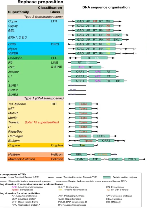
To stay consistent with previous literature on classification (Abrusan et al. 2005, Nakano et al. 2017, Nakano et al. 2018) I will classify TEs using the RepBase hierarchy as shown in figure 1.1. Repbase also annotates simple repeats (which includes satellites) and multicopy genes (which include tRNA, sRNA, and snRNA) . Statistics about the dataset are presented in Chapter 3, figure 3.1.
The largest division of TEs is between type I (retrotransposons) and type II (DNA transposons). This difference is primarily based on the how these two TEs move themselves across the genome. Type I TEs move through a “copy-and-paste” mechanism with an RNA intermediate while type II TEs transpose through a “cut-and-paste” mechanism with a DNA intermediate. Further TE classification is largely based on structural features related to protein domains and terminal repeats (long or inverted).
1.3 Thesis Statement
Short read classification is a competitive way of deriving the distribution of repetitive elements de novo in the genome. It is also possible to quickly ‘find’ sequences from real genomes which match a certain structure, like a repetitive element of interest, by learning an embedding for repetitive elements.
1.4 Organization
The organization of this thesis as follows:
Chapter 3: Presents the dataset and background to the specific classifiers used to classify transposable elements.
Chapter 4: Presents comparative results of classifying repetitive elements with various deep learning models versus sequence-based approaches.
Chapter 5: Presents work on unsupervised methods applied to generate reads from transposable elements.
CHAPTER 2: BACKGROUND
2.1 Introduction
In the past decade, deep learning has emerged as the workhorse of solving big data problems (I. Goodfellow et al. 2016). This status was quickly achieved through state of the art performance in the fields of image recognition, object detection, and natural language
processing. For each of these problems, specially designed deep learning networks were
constructed to most efficiently capture the intricacies of each set of data. For example, recurrent neural networks (RNN) are the primary tool used in text analysis while the sliding window approach of the convolutional neural network (CNN) has shown to be superior in image based problems. This modularity, as the availability of a rich set of flexible libraries to quickly implement deep learning models, has inspired a new wave of research in artificial intelligence.
The aim of this chapter is to present an overview of deep learning methods that will be used to analyze genomic data throughout this thesis. These include classical approaches like RNNs and CNNs, but also feature ways of learning metric space representations (triplet based deep learning), and unsupervised learning techniques.
2.2 Deep Learning Background
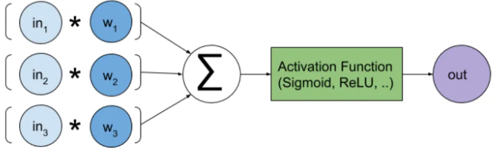
The neural network is a machine learning method that is capable of learning complex, nonlinear functions in a hierarchical manner using gradient-descent optimization. The functional unit of the neural network is a neuron, which has a single output for a set number of inputs k. Each input to a neuron, inputk, is multiplied by a weight, weightk, whose value is trained using gradient descent based optimization. Then, a sum is taken over all k weighted inputs, inputk * weightk. This is essentially a dot product between two vectors (one being the input and the other being the neuron weights). A nonlinear function (like sigmoid) is finally applied to this output value. The computation in a neuron on a set of inputs is illustrated in figure 2.1. A common nonlinearity used in current neural networks is the rectified nonlinearity (ReLU). The ReLU activation function clips the output of the neuron to be above 0, increasing sparsity and improving generalizability of the model. A problem with the ReLU activation function is that gradient information is lost for outputs less than 0. This problem can be alleviated with a ‘leaky’ variant of ReLU which sets outputs less than 0 to the output times a small constant. Common activation functions are shown in figure 2.2.
The input to a neural network layer is usually in the form of a batch of multiple samples. Figure 2.3 shows how running a batched input through a neural network layer can be efficiently represented as a matrix-matrix multiplication.
Figure 2.1: Visualization of neuron vector-vector multiplication based on weight parameters [w1, w2, w3] and input [in 1, in2, in3].
Figure 2.3: Visualization of the forward pass of a 3-sample batch through a 3-neuron layer as a matrix-matrix multiplication. Colors correspond to annotations in figure 2.1.
Experimentally, deeper networks have shown increased performance while retaining good generalizability (I. Goodfellow et al. 2016). Each layer also increases computational cost, so using very deep networks only became practical with the advent of GPU implementations of neural networks.
There is little restriction to how neural networks can be built, as long as all the operations are differentiable so that the parameters can be updated through back-propagation. Initially this led to extensive research into various activation functions, but newer developments tend to focus in how each layer ‘wires’ up to the next. For example, convolutional and recurrent networks were developed to exploit underlying input organization by enforcing a spatially aware way of processing inputs.
layer during training (Hinton et al. 2014). This forces nodes to learn parameters which can be applied in a multitude of different scenarios. Another proposal is batch normalization, which ensures each node does not have massive updates by making its output normally distributed with respect to each batch. The addition of batch normalization significantly improves learning rates and model generalizability, and has now become a standard drop-in layer for modern
convolutional networks (Ioffe and Szegedy 2015).
2.3 Current Repeat Element Classification
A problem with RepeatMasker is that it can have trouble classifying novel repeats not found in its library. De novo methods were made to discover and classify novel repeats based on structural characteristics which are derived from clues experts use to classify repeats. Once a consensus dataset of repeats has been derived from the sample, the next step for most of these methods is to check for protein domain conservation and indicative components like long
terminal repeats and terminal inverted repeats. As shown in figure 1.1, the presence and ordering of these components are defining characteristics of labeling repetitive elements. Once these features have been derived from the sequence, an expert-crafted rule-based system or an optimized machine learning classifier can be used to finally classify the repeat (Hoede et al. 2014). Previous deep learning approaches in the area have utilized k-mer counts as features rather than learning from the raw sequence (Nakano et al. 2017, Nakano et al 2018). Current de novo approaches rely heavily on accurate consensus sequences, which may be difficult to construct due to the nature of repetitive elements. For example, it is common for young TEs to insert within older TEs, which requires the accurate assertion of TE boundaries before the TE is classified (Joly-Lopez and Bureau 2018). Finally, these approaches are heavily reliant on
CHAPTER 3: CLASSIFIER EXPERIMENTAL SETUP
3.1 Introduction
This chapter introduces how I split the Repbase dataset to train and compare repeat element classifiers for fixed size kmer lengths. I review previous solutions to the classification problem as well as presenting new ones based on deep learning.
3.2 Dataset
The Repbase repeat database is a curated list of repeat element consensus sequences whose classes were discussed in Chapter 1. Classification is done based on the Repbase
hierarchy from figure 1.1, and additionally delineating LINE (R2, RTE, Jockey, L1, I) and SINE (tRNA, 7SL, 5S) elements. Three datasets were constructed from Repbase, which are called Update, Drosophila, and Aradiposis. The Update dataset consists of a train set from the RepBase 20.01 release and a test set from the current RepBase 24.01 release. The Aradiposis and
Figure 3.1: Class distributions and element length distributions for RepBase 24.01 and the datasets (aradiposis, drosophila and drosophila) derived from it. The total size for the train training and testing splits for each dataset were as follows: aradiposis (40925/466), drosophila (39413/2026), update (32112/9332).
from each consensus sequence in the training data set. Testing was conducted based on a 10 fixed, randomly chosen, kmers from each consensus in the test set.
3.3 Classifiers
The following section defines the deep learning classifier architectures that will be used in the experiments. An additional comparison will be made to RepeatMasker (RM) with default sequence comparison parameters (skipping bacterial insertion sequences checks, not masking RNA genes, and turning off tandem repeat finder) and use the training data sequences as a library to classify the repeats in the test data. Since the results of RM are subsequence detections of repeat element classes, classification of a sequence is based on the longest found match.
Some preprocessing was also done before feeding the dataset into each classifier. For sequence based models reliant on base pair (a, t, c, g) input, a one-hot representation is used and add an embedding layer directly before each of the networks. Some k-mer lengths were longer than some consensus sequences, so these were padded these with a one-hot representation of ‘n’ . Feature input was uniformly scaled to fit inputs between 0 and 1.0. A description of each of the deep learning models is as follows:
A problem with vanilla neural networks is that they do not utilize a beneficial prior over the space they learn. This is especially apparent when learning from images, where translational invariance fails to be learned quickly. The first example of neural network modularity was a response to this failure - the convolutional neural networks (CNNs) (Y. Lecun et al. 1998). CNNs utilize a sliding window approach where local neural network functions feed their output to neural networks with larger context at a higher level in the hierarchy, forcing the network into learning a function with translational invariance (an example of an infinitely strong prior). This greatly speeds up training time on image-based problems and massively reduces the number of parameters because each layer has extensive parameter sharing between kernels. Figure 3.2 visualizes how a CNN layer processes a 2d input. One can imagine a CNN as a single neuron with fixed context around itself being applied to every point in the image where its weight kernels fit.
Figure 3.2: Visualization of forward pass for a convolutional layer with a single kernel, where a normal convolutional layer would include many kernels. Though named a
Layer types which supplement convolutional layers have also developed, including ‘pooling’ layers which forego complex weight matrices in favor of a simple addition or maxing operation across inputs - helping to quickly reduce the size of the output features and increase context (A. Krizhevsky et al. 2012). Another type of layer is the residual layer, which helps gradients flow to the beginning of the network by adding the output of previous layers to those further in front (K. He 2015). Residual layers have allowed for unprecedented depth in deep networks , but at a certain point the accuracy tends not to improve by substantial margins over having a handful of layers (around 20-30).
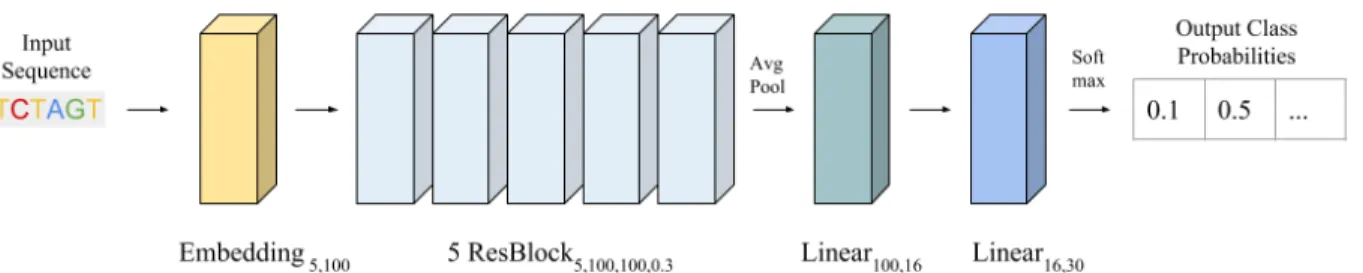
Residual Network (CNN): The reliable training, fast runtime, and ease of
interpretability of convolutional neural networks has seen the architecture become widely used for bioinformatics applications. Our architecture is motivated by the residual convolutional network used to train the DNA Generative Adversarial Networks in Killoran et. al. (2017) and Gupta et. al (2018). Figure 3.3 shows the architecture in detail. I found that for classification tasks it was important to add batch normalization before the activation functions in the residual blocks to stabilize training.
Recurrent neural networks (RNNs) also solve the problem of redundant local calculations by applying a ‘sliding window’ between a processed output from the last time step and the unprocessed input to the current timestep (Sherstinky 2018). The neural network structure which processes an individual timestep is commonly referred to as a cell. Figure 3.4 demonstrates how an RNN processes a sequence.
Figure 3.4: Visualization of forward pass for a simple recurrent layer with 3 neurons. Note that RNN cell flavors, like the LSTM or GRU, usually have more complicated function structures than the single vector-matrix multiplication and activation function shown here. Each color corresponds to annotations in figure 2.1.
self-loops. GRUs (Gated Recurrent Network) are another formulation which accomplishes the same task in a slightly different way, but achieves comparable results to the LSTM on most tasks. Further solutions to the exploding gradient problem include clipping the gradients at some constant, ensuring that extremely large gradients (which would cause inf or nan outputs) become tractable for the network to update its parameters on.
BiLSTM (RNN): Bi-directional LSTMs are a common choice for sequence analysis, especially in natural language processing. In this work I use a 2-layered, bidirectional LSTM with 128 nodes and a dropout of 0.5. The hidden states from the final layer are then average pooled across the sequence and run through a classifier with an intermediate layer of another 128 nodes and LeakyReLU activation. The final classification is done by a sigmoid output.
Each deep network based classifier is trained to minimize the cross entropy between output and real class labels. The adam optimizer is used with default parameters, namely with betas = (0.9,0.999) and epsilon = 10-8 . A learning rate of 0.1 was used. Every model was trained
CHAPTER 4: CLASSIFICATION RESULTS
4.1 Introduction
In this chapter I analyze the performance of each deep learning model with respect to speed, accuracy, and robustness to different kmer length scales. I also perform an analysis of kmers which may cause confusion at the read level. Then, I map the output of an intermediate layer to a low dimensional embedding space and attempt to learn a more useful embedding using a triplet loss.
4.2 Classification Results
This section presents the results of repeat element classification. The results indicate that deep learning methods are far faster and have greater generalizability to new repeat elements than sequence comparison methods, especially as hierarchy. I also show that K-mer count features have competitive testing accuracy with learning from a raw sequence string, although the count-based model suffers from a significantly worse fit on the training data.
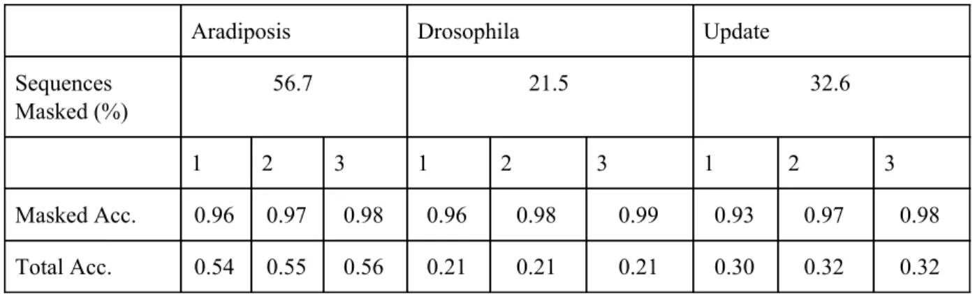
The first test measures the classification accuracy across the three datasets. Figure 4.1 and Figure 4.3 show the results of running repeatmasker on each of the datasets. Although repeatmasker was able to very accurately classify sequence for which it found matches, it was unable to find matches for a large portion of the sequences, resulting in overall lower
levels in the hierarchy, but deep learning models performed significantly better at higher levels. Repeatmasker did particularly well when the distribution of the testing dataset diverged from the distribution of the training data. This difference is especially apparent for the Aradiposis dataset, where there are far more Gypsy elements than Copia elements in the training dataset, but the other way around for the test data set. This is indicative of confusing sequences being mislabeled as the class which is present in higher number in the training dataset. The costs and benefits of such a model bias should be examined on a species specific basis. For example, in the
Drosophila dataset, this bias helped many more repeat elements be correctly classified by deep learning based methods. The update dataset seemed to be particularly difficult for both methods, resulting in the worst false positive rate for repeatmasker and the lowest classification accuracies for the deep learning models. We also compare precision, recall, and f1 scores for the
repeatmasker and deep learning models in figures 4.3 and 4.5.
Between deep learning models, the difference in classification is less pronounced, but overall the sequence based deep learning models (RNN and CNN) outperformed the DNN with kmer-count based features. The difference between the RNN and CNN models is less
pronounced, and in most cases negligible.
Aradiposis Drosophila Update
Sequences Masked (%)
56.7 21.5 32.6
1 2 3 1 2 3 1 2 3
Masked Acc. 0.96 0.97 0.98 0.96 0.98 0.99 0.93 0.97 0.98
Total Acc. 0.54 0.55 0.56 0.21 0.21 0.21 0.30 0.32 0.32
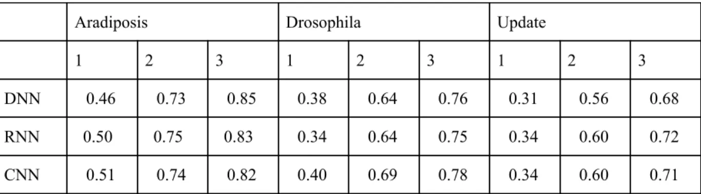
Aradiposis Drosophila Update
1 2 3 1 2 3 1 2 3
DNN 0.46 0.73 0.85 0.38 0.64 0.76 0.31 0.56 0.68
RNN 0.50 0.75 0.83 0.34 0.64 0.75 0.34 0.60 0.72
CNN 0.51 0.74 0.82 0.40 0.69 0.78 0.34 0.60 0.71
Figure 4.2: Testing accuracies of deep learning based methods on select repeat element datasets.
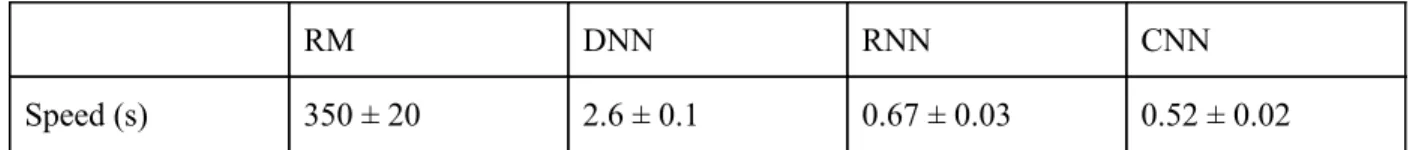
RM DNN RNN CNN
Speed (s) 350 ± 20 2.6 ± 0.1 0.67 ± 0.03 0.52 ± 0.02
Figure 4.4: Speed in seconds of running each classifier over 10,000 150-mers from the Repbase 24.01 dataset for 10 runs. Preprocessing, such as one-hot encoding and kmer counting, were included in the total times to simulate realistic usage.
Figure 4.5: CNN Precision, Recall and f1 Score for Aradiposis, Drosophila, and Update datasets.
k-mers than the deep learning models which require minimal preprocessing. The DNN model is slower mostly due to the time it takes to count k-mers. This time could likely be reduced with a more efficient implementation, but even so is far faster than sequence comparison methods.
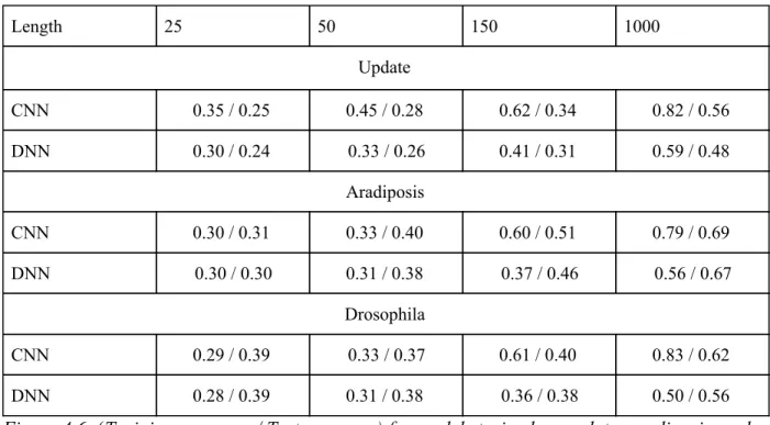
The third test examines differences between k-mer counts as features versus sequence input as we vary k-mer length. We selected lengths of 25, 50, and 150 as next generation sequencing technologies usually fragment the genome into reads of these lengths. The length of 1000 was included to show how much improvement could be expected in classification accuracy from very large read lengths and more accurate assembly of repetitive elements. Figure 4.6 shows that, as expected, having larger input sequences significantly improves model accuracy. Surprisingly, k-mer count features seem to be competitive with sequence input for testing on sequences derived from new species (Arabidopsis and Drosophila). When the sequences between the train and test datasets share greater similarity, as is seen in the Update dataset, models based on sequence based input show significantly better performance over kmer-count features. This is likely due to longer range k-mer features being available to use for the sequence based model, while the k-mer count model is reliant on very local signal.
To better understand how robust a trained CNN classifier is to picking different
classification, such as the boundary between two protein coding domains which indicates an element-specific ordering of protein domains.
Length 25 50 150 1000
Update
CNN 0.35 / 0.25 0.45 / 0.28 0.62 / 0.34 0.82 / 0.56
DNN 0.30 / 0.24 0.33 / 0.26 0.41 / 0.31 0.59 / 0.48
Aradiposis
CNN 0.30 / 0.31 0.33 / 0.40 0.60 / 0.51 0.79 / 0.69
DNN 0.30 / 0.30 0.31 / 0.38 0.37 / 0.46 0.56 / 0.67
Drosophila
CNN 0.29 / 0.39 0.33 / 0.37 0.61 / 0.40 0.83 / 0.62
DNN 0.28 / 0.39 0.31 / 0.38 0.36 / 0.38 0.50 / 0.56
Figure 4.6: (Training accuracy / Test accuracy) for models trained on update, aradiposis, and drosophila datasets when repeat elements are fragmented at varying kmer lengths. Each train/test accuracy is given at the lowest level in the RepBase hierarchy.
Figure 4.8: Log normalized confusion matrices of model on Update dataset.
4.3 Embedding Using Triplet Loss
The features learned by a neural network in classification tasks are optimized for
straightforward framework for metric space learning is the siamese network, in which pairs of samples are run through two copies of the same network (Koch 2015). The networks are punished for embedding pairs of inputs close to each other if they are from different classes or for embedding pairs of inputs far from each other if they are from the same class. Unfortunately, siamese networks can have stability problems with training reasonable embeddings in some scenarios (Hoffer and Ailon 2015). Triplet networks alleviated some of the training problems siamese network faced and significantly improved accuracy on face verification datasets. The triplet network takes a triplet of three samples, an anchor a, a positive sample p (which is meant to be similar to the anchor) and a negative sample (which is meant to be different). The same network is run for all three samples and the loss is calculated by the following triplet loss:
max (d (a, p) d (a, ) α, 0)
L = − n +
Where is a distance margin, and d is a distance function (normally an L2 loss).α
Figure 4.9: Visualization of triplet network structure with L2 based distance loss. Anchor, positive sample, and negative sample are given by a,p, and n. The same network f is applied to each of a, p, n. The margin is given by α .
t-SNE and PCA. I also attempt to improve the interpretability of the embedding by training a CNN model to reduce the distance between sequence pairs of different classes via a triplet loss.
CNN: This model is the same architecture as the previous CNN model and uses weights from the second to last layer, resulting in an embedding size of 16.
Triplet: I train a new model with the same architecture as the previous CNN model to optimize an L2 based triplet loss function enforcing a margin of 0.01.
Training parameters were the same as for the classification task. The triplet loss for the embedding from the CNN intermediate layer versus the triplet trained CNN model embedding are shown in figure 4.10. The new learned embeddings better abide by the triplet loss metric. To test the utility of the new embeddings, 100,000 kmers were embedded from the training sets of the Aradiposis, Drosophila, and Update datasets. A kd tree is used to quickly query the nearest neighbor in embedding space. Each testing sequence is then embedded and classified based on the nearest embedded neighbor from the training set.
Aradiposis Drosophila Update
CNN 0.0029 0.0025 0.0022
Triplet 0.000035 0.000032 0.000030
Figure 4.10. Triplet Loss with a margin of 0.01 from training set.
Although the new embeddings are better aligned with the triplet loss, they fare
Aradiposis Drosophila Update
1 2 3 1 2 3 1 2 3
CNN 0.49 0.68 0.79 0.27 0.56 0.71 0.24 0.54 0.63
Triplet 0.34 0.61 0.73 0.21 0.49 0.64 0.22 0.50 0.62 Figure 4.11. Accuracy of 1 nearest neighbors to 100,000 kmer training dataset.
There seems to be overall good separation of groups with many elements in both embeddings. For classes with fewer elements, t-SNE better brings out clusters than PCA. For example, the SINE elements in the t-SNE plots are clearly separated while they are scattered across other classes in the PCA embedding. The PCA embeddings for the raw CNN outputs are seen to be a less tightly grouped than the same embeddings trained on a triplet loss, but there is better separation of the hAT and Mariner elements than with the triplet loss embeddings. The t-SNE embedding shows little structural difference between the Triplet based and raw CNN embeddings.
Embeddings can be used for interpolating between sequences. For example, in figure 4.12 we interpolate between two gypsy sequences.
4.4 Conclusion and Discussion
In this chapter I conducted a comparative analysis of new and previously developed deep learning models with the sequence comparison based method repeatmasker. For classification of short sequences at the base of the RepBase hierarchy I find that repeatmasker achieves good testing accuracy with a low false positive rate. Higher up the RepBase hierarchy, or with longer sequence size, deep learning models can achieve more robust classification results which better warrant the approach. I experiment with sequence based and k-mer count input features and find that although kmer-count input features achieve competitive testing accuracy with sequence based models for shorter k-mer sizes, they fit the training data significantly worse for larger k-mer sizes and as such may have worse viability for classifying repeats with low divergence to the testing set. Then, I analyze embedding sequences based on the outputs of an intermediate layer of the deep learning model versus an embedding trained on the triplet loss. I compare the embeddings using visualization and nearest neighbor classification loss. I find that both
embeddings show good classification boundaries, but that using a triplet loss consistently decreases nearest neighbor classification accuracy.
The classifier results presented were also fine-tuned by increasing the number of layers and neurons per layer. Unfortunately, these changes did not result in significantly different classification results, indicating the need for either changing the input (for example, providing the context of all reads in a sample to the network), or applying an innovative network
CHAPTER 5: GENERATING REPEATS
5.1 Introduction
Previously I used supervised techniques to train classifiers on labeled dna sequences. Unsupervised techniques are a way of learning distinctive features of a dataset without needing these labels. Unsupervised deep learning presents an interesting way of learning likely TE mutations and variations, which may enable discovery of novel TEs. In this section I present a background to unsupervised deep learning techniques, like the autoencoder and Generative Adversarial Network, and discuss work using them to learn a class-specific embedding of repeat sequences.
5.2 Auto Encoders
function which penalizes unrealistic images. This motivated the development of generative adversarial networks (GANs) (Goodfellow 2014).
Another use for autoencoders is anomaly detection. Large differences between a
reconstruction and input sample can be used to detect areas of interest, for example, a tumor in a brain scan (Schlegl et al. 2019).
5.3 Generative Adversarial Networks
GANs are a modern take on unsupervised learning which learn to model a distribution by defining a competition between two neural networks (Goodfellow 2014). One network is labeled as the generator while the other is labeled as the discriminator. The generator’s goal is to fool the discriminator into being unable to distinguish between the set of real data and generated data, whilst the discriminator’s goal is to ensure generated samples are rejected and real samples are kept. The input to the generator is a sample from a normal distribution, meaning the generator is learning a function for mapping the samples of a probability distribution to realistic data
Figure 5.1: Comparison of generative adversarial network (GAN) and auto encoder (AE) architectures. The encoder, generator, and discriminator networks are labeled with e,g,and d respectively. The latent variable, or encoding of the sample, is given by z. Note that in the GAN, the latent z variable is generated by sampling a normal distribution.
Originally, Jensen-Shannon divergence was used to define the loss between the real and generated data distributions. Unfortunately, Jensen-Shannon divergence is prone to cases of gradient collapse which can ruin training and result in the generator only outputting noise. The Wasserstein GAN redefined the distribution distance function to an approximation of the earth mover distance (the minimum amount of effort needed to move one distribution into another), allowing for greater resilience to training problems ( Arjovsky et al. 2017, Gulrajani et al. 2017).
Recent work has explored the use of GANs for biological sequence data. Killoran et al. pretrained a generator to output realistic sequences before traversing the latent space to ‘design’ dna sequences with specific properties (Killoran et al. 2017) . This approach, however, requires a differentiable discriminator, which is not commonly available for most publicly available
5.4 Generation of Transposable Elements
Embeddings can be useful for interpolating between two sequences by looking at the nearest embedded neighbors. The quality of the interpolation is highly dependent on how many sequences are embedded, and may result in duplication (as seen in Figure 4.12) if a sequence is close to multiple interpolation points. To construct smooth interpolations, generative models must be used. One method to generate repeats is to use an autoencoder which minimizes the reconstruction loss between a real sequence and a generated output sequence. The most common generator network architecture that has been used with sequences up to 150 base pairs (Killoran et al. 2017, Gupta and Zhou 2018) is shown in Figure 5.1, which is similar to the classifier trained in the previous section.
Figure 5.1. Residual network decoder/generator used in this work. The initial linear layer takes as input a 128 dimensional embedding of a DNA sequence and outputs a length 150 vector (the length of the DNA sequence to be generated). The residual blocks are defined as in figure 3.3. Note that the initial linear layer embedding size is varied, since accurate reconstruction from a size 16 embedding was troublesome.
found that training an autoencoder on repetitive elements without learning to memorize the input required a few model tweaks. First, I tested the following embedding sizes: [32, 64, 128].
Embedding sizes larger than 128 were not tested since the model could learn to memorize the input perfectly at an embedding size of 128 (>99% reconstruction accuracy on held out sequence classes). Embedding sizes smaller than 128 consistently had trouble training, so I opted to keep this embedding size and teach the network to denoise inputs by randomly changing [10,20,40] of the 150 input base pairs. The networks consistently trained to the maximum accuracy that could be achieved by copying the input and then stabilized. These problems echo those stated in Killoran et al (2017). Schegl et al (2019) showed an improvement to autoencoders by first training a GAN on the samples, freezing the GAN and then training an encoder network to learn a mapping from a real sample to a latent variable. I was able to successfully train the Wasserstein GAN from Killoran et al to output realistic sequences as can be seen in figure 3.16.
Unfortunately, using the method of Schegl et al, the encoder network was not able to learn a reasonable mapping from sequences to the latent vector and had a base-pair reconstruction accuracy of only 40% for LTR sequences (which the GAN and encoder were trained on) and 39% for non-LTR sequences (which were used as the test set).
Figure 5.2. Example interpolation of two points in latent space by WGAN model trained on LTR Sequences.
Figure 5.3. Similarity using Levenshtein edit distance metric between randomly generated SINE reads (blue) versus SINE reads generated by GAN (Orange) and real SINE reads. Similarity is taken between reads from a randomly excluded SINE element versus reads from other SINE elements not chosen.
5.5 Conclusion and Discussion
CHAPTER 6: WEB TOOLS AND CONCLUSION
As a complement to this work, I also developed a web application for utilizing some of the models present in this thesis. I built the application in flask and React. Capabilities of the application include returning the classification of a sequence, showing the repeat distribution of a set of k-mers, and the class probability at each point in the k-mer by using the classifier as a sliding window. I also enable visualizations of the query k-mers in PCA space. Finally, the application enables users to see the output of the GAN model I trained on repeat elements, nearest neighbors of select embedded training sequences, and interpolation between sequences in latent space.
In this work I utilized deep learning techniques to train a classifier on short read-like sequences from repeat elements. I showed that an initial classification of such sequences is possible to perform far more quickly using deep learning techniques, although with a loss in precision. Finally, I experimented with different ways of learning an embedding space for
sequences, and showed that the intermediate layer output of the classifier worked well when used to classify nearest neighbors in the test set. In future work I will continue to work on
REFERENCES
G. Abrusan, N. Grundmann, L. DeMester, and W. Makalowski “TEclass - a tool for automated classification of unknown eukaryotic transposable elements” Bioinformatics Applications Note
200: 25(10) : 1329-1330
M. Arjovsky, S. Chintala, and L. Bottou “Wasserstein GAN” Arxiv:1701.07875 2017
W. Bao, K.K. Kojima, and O. Kohany “Repbase Update, a database of repetitive elements in eukaryotic genomes” Mob DNA, 2015;6:11
X. Cui, P. Jin, et al. “Control of Transposon activity by a histone H3K4 demethylase in rice. “
Proc Natl Acad Sci U S A. 2013;110(5):1953-8.
S. R. Eddy “Multiple Alignment Using Hidden Markov Model” Proc. Third Int. Conf. Intelligent
Systems for Molecular Biology 1995:114-120
A. Gupta and J. Zou “Feedback GAN (FBGAN) for DNA: A Novel Feedback-loop Architecture for Optimizing Protein Functions” Arxiv:1804.01694 2018
S. Goswami, K. Lee, S. Shams and S. Park, "GPU-Accelerated Large-Scale Genome Assembly,"
2018 IEEE International Parallel and Distributed Processing Symposium (IPDPS), Vancouver, BC, 2018, pp. 814-824. doi: 10.1109/IPDPS.2018.00091
I. Gulrajani , F. Ahmed, M. Arjovsky, V. Dumoulin, A. Courville “Improved training of Wasserstein GAN” Arxiv:1704.00028 2017
I. Goodfellow, Y. Bengio, and A. Courville “Deep Learning” MIT Press 2016
C. Hoede, S. Arnoux, M. Moisset, et al. “PASTEC: AN Automatic Transposable Element Classification Tool.” PLOS One 2014
E. Hoffer and N. Ailon “Deep Metric Learning using Triplet Network” ICLR 2015 I. Goodfellow “Generative Adversarial Nets” NIPS 2014
P. J. Hornsby “Telomerase and the aging process” Experimental gerontology vol. 42,7 (2007): 575-81.
G.E. Hinton, N.Srivastava, A.Krizhevsky, I. Sutskever, and R. R. Salakhutdinov “Dropout: A simple Way to Prevent Neural Networks from Overfitting” JMLR, 2014 vol 15:1929−1958 R. Hubley, R.D. Finn, J. Clements, et al. “The Dfam database of repetitive DNA Families”
Nucleic Acids Res 2015; 44(D1): D81-9
S. Ioffe and C. Szegedy “Batch Normalization: Accelerating Deep Network Training by Reducing Internal Covariate Shift” Arxiv:1502.03167 2015
V. Jamilloux, J. Daron, F. Choulet, and H. Quesneville “De Novo Annotation of Transposable Elements: Tackling the Fat Genome Issue” IEEE vol 105, 3 (2016)
Z. Joly-Lopez and T. E. Bureau “Exaptation of Transposable element coding sequences”
Genetics and Development 2018; 49:34-42
K. K. Kojima “Human Transposable Elements in Repbase: Genomic Footprints from Fish to Humans” Mobile DNA (2018); 9(2)
N. Killoran, L.J. Lee, A. Delong, D. Duvenaud and B. J. Frey “Generating and designing DNA with deep generative models” 2017 arXiv:1712.06148v1
G. Koch, R. Zemel, R. Salakhutdinov “Siamese Neural Networks for One-shot Image Recognition” 2015
G. Koch “Siamese Neural Networks for One-Shot Image Recognition” University of Toronto Master’s Thesis 2015
A. Krizhevsky, I. Sutskever, and G. Hinton “ImageNet Classification with Deep Convolutional Neural Networks” NIPS 2012
Y. Lecun, L. Bottou, Y. Bengio, and P. Haffner “Gradient-Based Learning Approach to Document Recognition” IEEE Proceedings 1998
F. K. Nakano, W.J. Pinto, G. L. Pappa, and R. Cerri “Top-down Strategies for Hierarchical Classification of Transposable Elements with Neural Networks” IEEE 2017
F.K. Nakano, S. M. Mastelini, S. Barbon, and R. Cerri “Improving Hierarchical Classification of Transposable Elements using Deep Neural Networks” IEEE 2018
B. Piegu, S. Bire, P. Arensburger, Y. Bigot “A Survey of Transposable Element Classification Systems - A call for a fundamental update to meet the challenge of their diversity and
complexity” Molecular Phylogenetics and Evolution 2015: 86 :90-109
D. Rodriguez-Terrones and M.E. Torres-Padilla “Nimble and Ready to Mingle: Transposon Outbursts of Early Development” Trends in Genetics vol 34,10 (2018)
L. Schrader and J. Schmitz “The impact of transposable elements in adaptive evolution”,
Molecular Ecology (2018): 1-13
T. Schlegl, P. Seebock, S. Waldstein, G. Langs, and U. Schmidt-Erfurth “f-AnoGAN: Fast unsupervised anomaly detection with generative adversarial networks” Medical Image Analysis 2019
A. Sherstinsky “Fundamental of Recurrent Neural Network (RNN) and Long Short-Term Memory (LSTM) Network” Arxiv:1808.03314 2018
A. Smit, R. Hubley and P. Green. RepeatMasker Open-4.0. 2013-2015
<http://www.repeatmasker.org>
T.J. Treangen and S.L. Salzberg Repetitive DNA and next-generation sequencing: computational challenges and solutions. Nat Rev Genet. 2011;13(1):36-46. doi:10.1038/nrg3117
T. J. Wheeler, J. Clements, S.R. Eddy, et al. “Dfam: a database of repetitive DNA based on
profile hidden Markov models.” Nucleic Acids Res. 2012;41(Database issue):D70-82.