1220.pdf

'^w^g^lf-ALLEN MARTIN MABRY. Radon-222 Concentrations in North Carolina

Household Groundwater Supplies (Under the direction of JAMES E.

WATSON, JR.)

A survey of randomly selected households served by

groundwater was conducted to characterize radon-222 concentrations

in groundwater-derived drinking water supplies in North Carolina.

Groundwater sources in North Carolina had previously been analyzed

for radon-222 by other researchers, but a random survey had never

been attempted. The investigation included regional comparisons of

radon-222 concentrations, characterization of the distribution of

concentrations, and a comparison of the indoor airborne

One hundred and seventy-four homes were successfully

surveyed. The statewide average concentration was 2,229 pCi/1.

The eastern region of the state had a markedly lower average

concentration of 337 pCi/1. Sixty-eight percent of the measured

concentrations were above the U.S. Environmental Protection

Agency's proposed maximum contaminant level of 300 pCi/1. The

comparison of indoor airborne concentrations to waterborne

ill

Table of Contents

Page

I. INTRODUCTION... 1

Physical Properties of Radon-222... 1

Occurrence of Radon in Drinking Water... 1

North Carolina Data... 4

Health Risks... 4

Proposed Regulation... 7

II. MATERIALS AND METHODS... 9

Participant Selection... 9

Sampling Procedure... 10

Sample Analysis... 10

Determination of State and Regional Averages... 15

III. RESULTS... 18

Distribution of Results... 19

Regional Comparisons... 25

Comparison with the EPA's MCL... 27

Air Concentration Versus Water Concentration... 28

Comparison of Duplicate Samples... 28

Discussion... 31

Conclusions... 33

REFERENCES... 34

APPENDIXES... 36

A. Instructions... 36

B. Packard Tri-Carb 300 LSC Program Settings... 37

C. Background Values... 38

D. Standard Counts and Calibration Factors... 40

iv

List of Tables

Page

1. Principal Decays from U-238 to Pb-206... 2

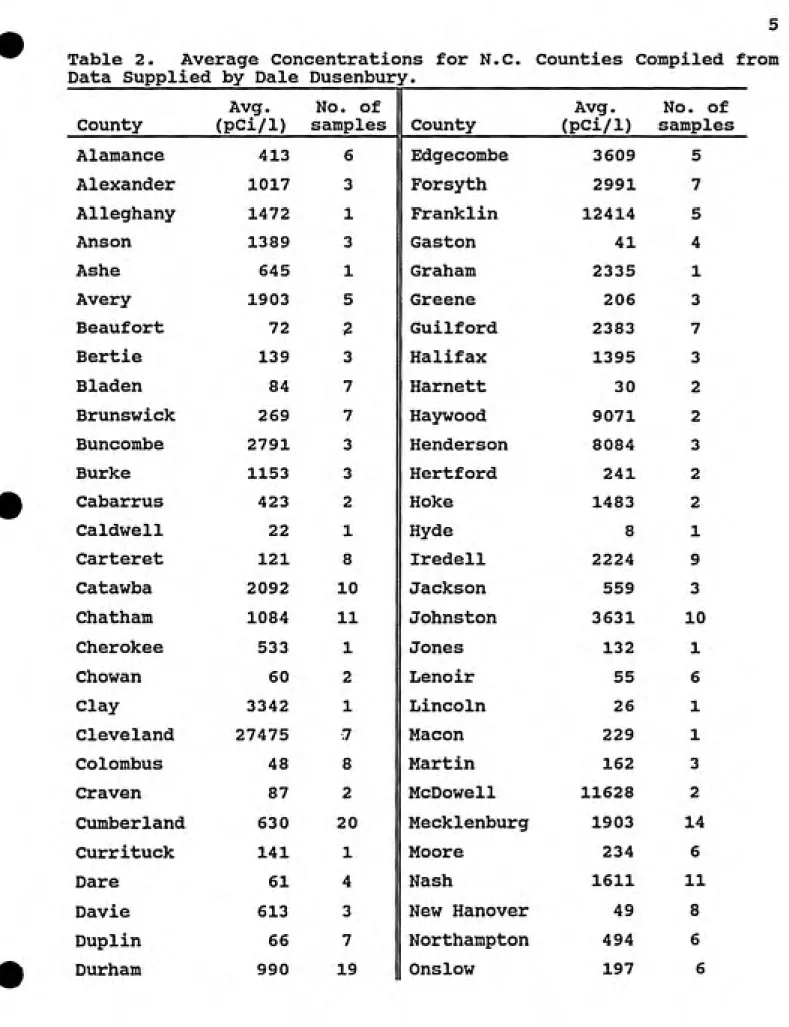
2. Average Concentrations for N.C. Counties Compiled

from Data Supplied by Dale Dusenbury... 5

3 . Summary of Results... 19

List of Figures

Page

1. Map of the three regions of comparison... 17

2 . Map of the counties sampled... 17

3. Frequency distribution of the concentrations

between 0 and 10,000 pCi/1... 20

4. Frequency distribution of concentrations on a log

scale... 21

5. Frequency distribution of concentrations in the

eastern region on a log scale... 22

6. Frequency distribution of concentrations in the

central region on a log scale... 23

western region on a log scale... 24

8. Box plots for the three regions... 26

concentration with a linear regression overlaid.... 29

10. Frequency distribution of the percent

INTRODUCTION

This project was undertaken to achieve two objectives: (1) to

obtain a representative characterization of radon-222 concentra¬

tions of North Carolina groundwater sources used for drinking

water, and (2) to compare radon-222 concentrations in groundwater

sources to the airborne radon-222 concentrations in the homes

served by them.

Physical Properties of Radon-222

Radon-222 (henceforth radon) is a radioactive noble gas that

occurs naturally as a product of the decay of radium, a member of

the uranium series of radionuclides, which is present in most soils

(BEIR 1988). Radon decays by alpha particle emission with a

half-life of 3.82 days to the solid daughter Po-218. Po-218 decays to

Pb-214 by alpha emission; Pb-214 decays to Bi-214 by beta emission.

Bi-214 then decays to Po-214 by beta emission; Po-214 decays almost

instantaneously by alpha emission to the long-lived daughter

Pb-210. This decay series is shown in Table 1. Eguilibrium of the

short-lived daughters with the parent is reached in about 3 hours

(Evans 1969).

Occurrence of Radon in Drinking Water

Table 1. Principal Decays from U-238 to Pb-206 (ICRP 1983) Isotope Half-life Principal radiation Principal alpha energies (MeV) Principal gamma energies (MeV)

U-238 4.5x10^ y alpha 4.198 4.149

(77%)

(23%) Th-234 24.1 d beta

Pa-234m 1.17 min beta

U-234 _{244,500 y} alpha 4.773 4.721

(72%) (27%)

Th-230 _{77,000 y} alpha 4.688 4.621

(76%) (23%)

Ra-226 1,600 y alpha 4.785

4.602

(94%)

(6%) Rn-222 3.82 d _alpha 5.490 _(100%) Po-218 3.05 min alpha 6.003 _(100%)

Pb-214 26.8 min beta gamma

0.2952 (19%)

0.3519 (37%)

Bi-214 19.9 min beta gamma

0.6093 (46%) 1.120 (15%) 1.765 (16%)

Po-214 1.6x10"^ s alpha 7.687 (100%)

Pb-210 22.3 y beta

Bi-210 5.01 d beta

Po-210 138 d alpha 5.297 (100%)

3

varying amounts (EPA 1984). The U.S. Environmental Protection

Agency (EPA) estimates an average U.S. drinking water radon

concentration in the range of 200 to 600 pCi/1 for groundwater

sources. The EPA estimates that the majority of water supplies

served by groundwater have concentrations less than 2,000 pCi/1

(Milvy and Cothern 1990). Radon is not typically found in surface

water sources, and larger public groundwater systems usually have

lower concentrations of radon than smaller systems and private

wells (Milvy and Cothern 90) . A concentration of 750,000 pCi/1 has

been measured in one public water supply (Milvy and Cothern 1990),

and a concentration of 3x10* pCi/1 has been measured in a private

well in Colorado (Lawrence et al. 1992).

An analysis of available radon concentration data performed

by C.T. Hess et al. combined the results from 6,298 samples taken

from U.S. public groundwater supplies and calculated a geometric

mean of 130 pCi/1. In the same study, the results from 454 samples

taken from private wells in the United States had a geometric mean

of 920 pCi/1 (Hess et al. 1985) . The National Inorganics and

Radionuclides Survey (NIRS) randomly surveyed 978 U.S. community

groundwater supplies. Of the systems surveyed, 48% had radon

concentrations greater than 200 pCi/1. Population-weighted

averages of 249 and 2,277 pCi/1 for the United States and North

Carolina, respectively, were obtained from the survey. The smaller

systems that were surveyed averaged higher radon concentrations.

The population-weighted average for U.S. systems serving fewer than

4

North Carolina Data

Radon concentrations in N.C. groundwater sources have been

reported by the EPA, the N.C. Division of Radiation Protection, and

the University of North Carolina. A compilation of 437 sample

results obtained from those sources has been prepared by Dale

Dusenbury (Dusenbury 1992). Concentrations range from 0 to 55,900

pCi/1, with an average of 2,430 pCi/1. County averages computed

from those concentrations are shown in Table 2. A high degree of

variability throughout the state is evident. These samples were

not randomly obtained, and not all of them were from drinking water

sources.

Regional variations in average radon concentrations in water

associated with different rock types have been reported (Loomis

1987) . It has also been shown that geologic region is a good

predictor of radon concentration in North Carolina (Loomis et al.

1987).

Health Risks

The presence of radon in groundwater presents a health risk

to the public. Compared with all other naturally occurring

radionuclides present in drinking water, radon presents the

greatest health risk (Milvy and Cothern 1990). Two routes of

exposure are possible from waterborne radon: ingestion of the

Table 2. Average Concentrations for N.C.

Data Supplied by Dale Dusenbury.

Counties Compiled from

County

Avg.

(pCi/1)

No. of

samples

1 County

Avg.

(pCi/1)

No. of

samples

Alamance 413 6 Edgecombe 3609 5

Alexander 1017 3 _Forsyth 2991 7

Alleghany 1472 1 Franklin 12414 5

Anson 1389 3 Gaston 41 4

Ashe 645 1 Graham 2335 1

Avery 1903 5 Greene 206 3

Beaufort 72 2 Guilford 2383 7

Bertie 139 3 Halifax 1395 3

Bladen 84 7 Harnett 30 2

Brunswick 269 7 _Haywood 9071 2

Buncombe 2791 3 Henderson 8084 3

Burke 1153 3 Hertford 241 2

Cabarrus 423 2 Hoke 1483 2

Caldwell 22 1 _Hyde 8 1

Carteret 121 8 Iredell 2224 9

Catawba 2092 10 Jackson 559 3

Chatham 1084 11 Johnston 3631 10

Cherokee 533 1 Jones 132 1

Chowan 60 2 Lenoir 55 6

Clay 3342 1 Lincoln 26 1

Cleveland 27475 7 Macon 229 1

Colombus 48 8 Martin 162 3

Craven 87 2 McDowell 11628 2

Cumberland 630 20 _Mecklenburg 1903 14

Currituck 141 1 Moore 234 6

Dare 61 4 Nash 1611 11

Davie 613 3 New Hanover 49 8

Duplin 66 7 _Northampton 494 6

Table 2 (continued)

County

Avg.

(pCi/1)

No. of

samples County

Avg.

(pCi/1)

No. of

samples

Orange 1118 8 Stanly 1198 5

Pamlico 40 3 Stokes 2264 4

Pasquotank 27 1 Surry 2067 16

Fender 29 2 _Transylvania 8377 2

Perquimans 120 2 Tyrrell 95 2

Pitt 89 5 Union 1755 1

Polk 11 2 Vance 6797 2

Randolph 278 4 Wake 6540 30

Robeson 50 6 Warren 9580 6

Rockingham 4126 12 _Watauga 1296 3

Rowan 1670 8 _Wayne 610 10

Rutherford 5350 5 Wilkes 946 2

Sampson 71 3 Wilson 1310 6

Scotland 343 1 Yadkin 1167 2

lung cancer risk due to inhalation because of the experiences of

uranium miners (NCRP 1984).

7

inhaled under typical conditions (Cross et al. 1985). However, risk comparisons based on calculations of absorbed dose vary, and it has been suggested that ingestion may be a significant exposure

pathway for waterborne radon (Crawford-Brown 1990).

Proposed Regulation

Currently, the radon concentration of drinking water is not

regulated. The EPA has proposed a maximum contaminant level (MCL)

of 300 pCi/1 based primarily on the inhalation risk from the

contribution of the waterborne radon to the airborne radon

concentration (EPA 1991). Previous studies indicate a waterborne

concentration of 10,000 pCi/1 would contribute an additional

1 pCi/1 to the indoor air concentration of a typical household

(Hess and Beasley 1990). The proposed MCL would affect an

estimated 26,000 public water supply systems in the United States

(EPA 1991). Private wells are not regulated by EPA drinking water

concern prompts the mortgage industry to adopt the MCL as a

standard (Barren 1990) . Removal of radon from water is achievable

with currently available processess. Granular activated carbon

radon in water processed (Lowry 1988).

A radon concentration of 300 pCi/1 in a household water

8

of the household based on a water-to-air transfer factor of 10^.

Lifetime continuous exposure to this concentration yields an

additional lifetime risk of lung cancer mortality of 1.8 x 10"*

based on a risk factor of 350 cancer deaths per 10* Person Working

Level Months, assuming 50% equilibrium of the radon daughters with

the radon and 70 years of exposure (BEIR 1988). A Working Level is

a radon concentration unit equal to 100 pCi/1 of radon in air at

100% equilibrium with the daughters.

By randomly surveying groundwater supplies, it was intended

to investigate the scope and magnitude of radon contamination in

N.C. drinking water supplies derived from groundwater. It was also

intended to determine what percentage of households might be

affected by the EPA's proposed MCL of 300 pCi/1. The comparison of

airborne radon concentrations to waterborne concentrations was not

intended to determine the rate of transfer of radon from water to

air since there are overshadowing contributions to indoor air

concentrations. Instead, the comparison was undertaken to

investigate the possibility of an association between airborne and

MATERIALS AND METHODS

Participant Selection

An address list of participants in the State/EPA survey of

residential indoor air radon concentrations in North Carolina was

obtained from Dr. Felix Fong of the N.C. Division of Radiation

Protection. The State/EPA survey, completed in 1990, randomly

sampled 1,290 residences throughout North Carolina. As part of the

survey those homes served by well water were identified. Five

hundred and eighty-four homes that used well water were included in

the survey.

It was not certain at the beginning of the project whether it

would be feasible to survey all 584 homes with well water.

Therefore, an approach was employed in selecting participants from

the list to preserve the randomness of the survey. Numbers

representing a random ordering of the participants had been

assigned to each participant of the State/EPA survey during the

random selection process. Therefore, participants were chosen in

ascending order according to these numbers.

Sampling was performed in groups of 25 homes each to keep the

processing of samples manageable. Home owners were mailed letters asking them to participate in the survey. If they did not refuse the request, they were mailed a sampling kit. From November 1990 through February 1991, 250 home owners were surveyed in this

10

Sampling Procedure

The sampling kit consisted of a cardboard mailing tube

containing two 20-ml scintillation vials containing 10 ml each of

liquid scintillation counting (LSC) cocktail, instructions for

collecting samples (see Appendix A) , packing material, and a return

address label with postage affixed.

The scintillation vials with LSC solution were preweighed and

marked with unique identification numbers. The scintillation vial

used was a polyethylene cone-capped, glass vial, available from

Fisher Scientific (part no. VWR 66022-128), that had been found to

be a suitable vial for containing radon gas (Hess and Beasley

1990). The scintillation cocktail used was a mineral oil-based

cocktail available from E. I. du Pont NEN (High Efficiency Mineral

Oil Scintillator part no. NEF 957A).

The participants were instructed to choose a faucet in the

home that did not have any attachments, like an aerator, or to

remove the attachment from a faucet if necessary. They were to let

the cold water run for 5 minutes, reduce the flow, then fill each

vial to the neck, capping it immediately. They were instructed to

record the date and time the samples were taken on the instruction

sheet and to return the samples and sheet promptly.

Sample Analysis

When samples were received at XJNC, the volume of water

collected was determined by weighing the samples and then

11

assuming a density of water equal to 1 gram/ml. The dates and

times of sample collections provided by participants were recorded.

Each vial was shaken vigorously for 15 seconds to extract the radon

from the aqueous phase into the organic scintillator phase of the

mixture. After the extraction process, counting was delayed for at

least 4 hours to allow the radon daughters to reach equilibrium

with the radon. Counting was performed with a Packard Tri-Carb 300

liquid scintillation counter. The counter was programmed to count

each vial for either 50 minutes or until 2 standard deviations of

the gross count equaled 2% of the gross count, whichever came

first. See Appendix B for details of the counting procedure.

Two background vials, each containing 10 ml of scintillator

fluid and 10 ml of distilled water, were counted with each batch of

samples. The two background count rates thus obtained were

averaged for each batch of samples. The background values for the

39 batches counted during the survey are presented in Appendix C.

The background values ranged from 29.83 to 32.50 cpm with an

average value of 31.19 cpm and a standard deviation of 0.79 cpm

(2.5%).

Two standard activity vials were counted with each batch of

samples; they were sealed aqueous radium-226 standards of 714 and

952 pCi (Ladrach 1987). Before counting, the standards were shaken

and allowed approximately 4 hours to reach equilibrium in the same

manner as described above for samples. The 4-hour delay was

!^^^»^^B?apsiaM^*i^^

12

and three additional empty vials, which totalled 250 minutes. The

two standard count rates thus obtained were used to determine an

average calibration factor for each batch of samples. A decay

correction was not necessary for this calculation because the

standards were counted about 4 hours from the time they were

shaken. Additionally, it was observed that the measured count

rates of the standards did not decrease with time, suggesting that

the transfer of the radon to the scintillation cocktail was

continuous and independent of the shaking process previously

described. For example, on one occasion the counter malfunctioned

and counted the standards and samples for 13 repetitions over a

54-hour period, and no significant change in the count rates of the

standards occurred. This phenomenon was also observed by EPA

researchers (EPA 1990). The calibration factors for the 39 batches

of samples processed during the survey are presented in Appendix D.

The average calibration factor was 10.0 cpm/pCi, with a standard

deviation of 0.14 cpm (1.4%). The calibration factors ranged from

9.68 to 10.26 cpm/pCi.

Radon concentrations in pCi/1 were calculated from the net

count rates by applying the calibration factor and correcting the

results for decay. The following relationship was used:

13

where:

K = calibration factor (cpm/pCi) V = sample volume (ml)

X = physical decay constant for radon (0.18 days"^)

t = elapsed time between sample collection and analysis

(days)

The concentrations of the two samples obtained from each home were

averaged to determine the concentration for each home. These

average concentrations were reported to the participants by mail.

The standard deviation of the count rate (a) for each result was

calculated based on the standard deviations of the sample and

background count rates using error propagation formulae.

It was necessary to determine the level below which a result

was more likely to be due to statistical fluctuation of the

background than to true radioactivity in the sample. The decision

limit for nondetection was calculated using the relationship given

in NCRP Report No. 58:

Lc = K yf2 ^/B = l.SA. y/2 yfB = 2.32 y/B

where:

Lc= decision limit, net counts

(95% confidence level)

K = 1.64

14

The decision limit is the net number of counts at which there

is 95% probability that any signal below it is false detection.

The complement to the decision limit is the detection limit given

in NCRP Report No. 58:

Ln = K^ + 2 L^ = 2.71 + 4.65 /S

where:

Li,= detection limit, net counts (95% confidence level)

K = 1.64

B = background counts Lc= decision limit

The detection limit is the net number of counts at which there is

95% confidence that a signal above it will be detected.

The decision limit was calculated for each batch of samples

using the background count for that day. For example, a background

count rate of 32.0 cpm obtained over a 50-minute count (1,600 total

counts) would yield:

r = 2.32 y/^'^P^ =1.86 cpm

For a typical 10 ml sample taken 4 days prior to counting and

ͣ 'yy^s=

15

concentration would be determined using the previously given

relationship for calculating concentration as follows:

Lc = (1.856 cpm) ^ / . ^°°° ^y-^ e-'2 = 34 ci/1

Results below the decision limit were so noted, but not discarded.

Discarding values would introduce bias into calculated averages.

Determination of State and Regional Averages

State, regional, and county averages were determined after

applying weighting factors to all results based on infoirmation

supplied with the State/EPA survey data base. The weighting

factors were necessary because the State/EPA survey used different

sampling rates across the state to favor areas of greater interest.

The weighting factors also incorporated other minor adjustments

that resulted from the participant selection process (personal

communication with Dr. Jane W. Bergsten of Research Triangle

Institute).

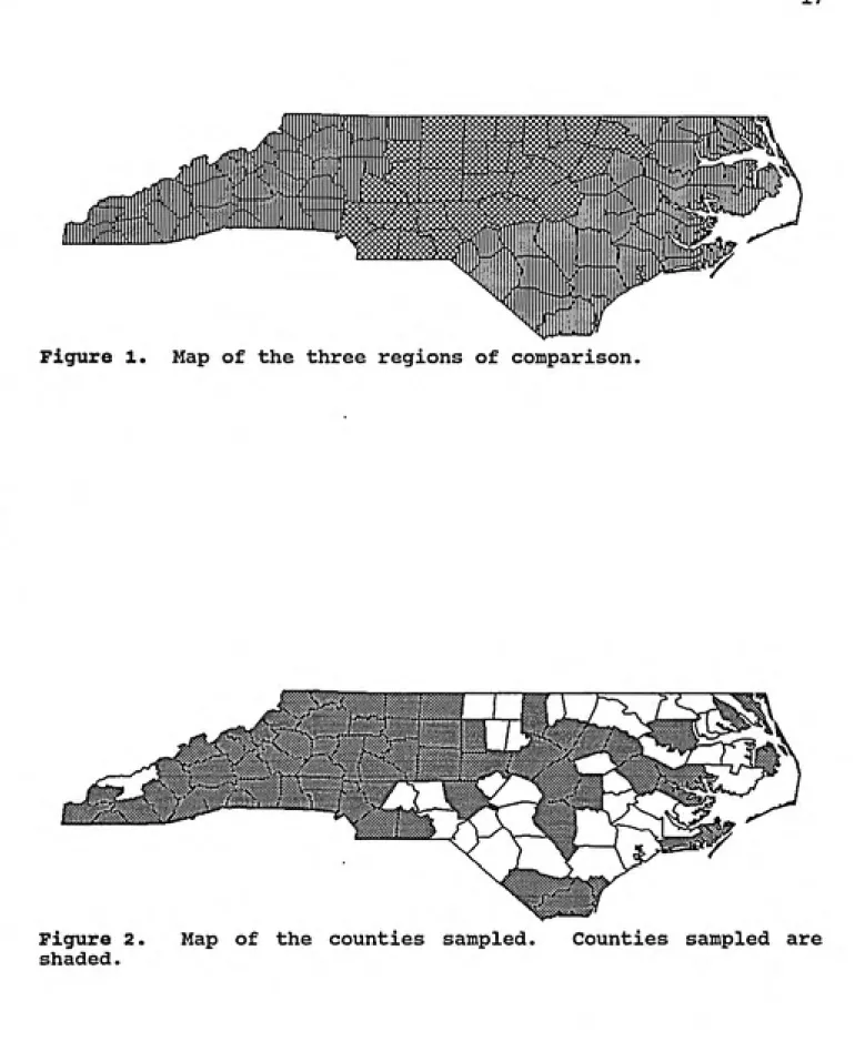
The division of the state into the three regions used in this

study is shown in Fig. 1. The counties that were sampled are shown

in Fig. 2. The division of the state was based on geologic regions

which have been shown to be predictors of radon concentration

(Loomis et al. 1987). The eastern region represents the Coastal

16

Belt, and Raleigh Belt, and the western region is composed of the

17

Figure 1. Map of the three regions of comparison.

A

Figure 2

shaded.

18

RESULTS

Two hundred and fifty homes were originally selected for

sampling. Ten of those were eventually determined to be ineligible

for the study. Ineligible homes included those that responded back

that groundwater was not used and those for which the sample

mailers were returned by the post office as undeliverable. At the

conclusion of the sampling phase, 174 residential groundwater

samples had been collected and analyzed. The collection success

rate was 73% for eligible homes. Samples not collected from

eligible homes were a result of no response by the home owner.

Duplicate samples were requested from each home owner. Of

the 174 homes surveyed, 162 were successfully sampled in duplicate.

Sample pairs received that had one broken vial resulted in singular

samples for 12 of the homes surveyed. The concentration for each

dually sampled home was determined by averaging the concentrations

of the two samples.

The results are listed in Appendix E. The unweighted average

concentration for all samples was 2,298 pCi/1. The weight-adjusted

average concentration for the state was 2,228 pCi/1. The eastern

region of the state had the lowest weight-adjusted average

concentration, 337 pCi/1; the central and western regions had

higher weight-adjusted average concentrations of 3,524 and 2,371

pCi/1, respectively.

A summary of the results is presented in Table 3. Measured

19

presented in this section represent weight-adjusted values. The

results listed in Appendix E are without any adjustments.

Table 3. Summary of Results

Region Number Minimum Maximum _Weighted

mean

Weighted

median

Eastern 24 71 _1,715 337 246

Central 31 55 _19,558 3,524 945

Western 119 21 _59,088 2,371 1,191

State 174 21 _{59,088 2,229} 570

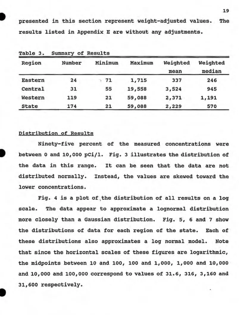
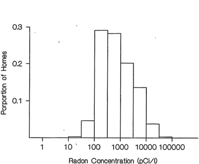
Distribution of Results

Ninety-five percent of the measured concentrations were

between 0 and 10,000 pCi/1. Fig. 3 illustrates the distribution of

the data in this range. It can be seen that the data are not

distributed normally. Instead, the values are skewed toward the

lower concentrations.

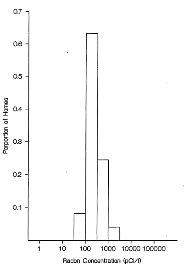
Fig. 4 is a plot of the distribution of all results on a log

scale. The data appear to approximate a lognormal distribution

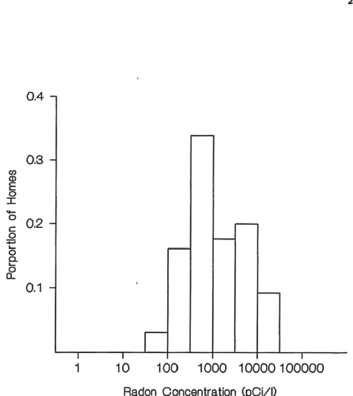
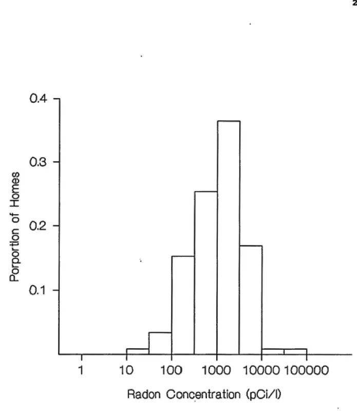
more closely than a Gaussian distribution. Fig. 5, 6 and 7 show

the distributions of data for each region of the state. Each of

these distributions also approximates a log normal model. Note

that since the horizontal scales of these figures are logarithmic,

the midpoints between 10 and 100, 100 and 1,000, 1,000 and 10,000

and 10,000 and 100,000 correspond to values of 31.6, 316, 3,160 and

20

0.7 n

0.6

-0.5

to

I 0.4

X

c

o

a 0,3

0.2

-0,1

0 2000 4000 6000 8000 10000

Radon Concentration (pCi/l)

21

0,3

CO

Q

o 0.2 X

o c

g

-1—>

a 0,1

o

a.

10 ͣ 100 1000 10000 100000

Radon Conoentration (pCi/l)

0.7 n

22

0.6

0.5

-CO

CD

o 0.4 H

X

R 0.3

0.2

0.1

-T 10 100 1000 10000 100000

Radon Concentration (pCi/l)

23

0.4 -1

0,3

CD

E

o

X

g

o ci

i_

o

0.2

0.1

-10 100 1000 10000 100000

Radon Conoentration (pCi/l)

24

CO

O

E

o

X

4—

o

c

o

o o

CL

0.4

0.3

0.2

-0.1

10 100 1000 10000 100000

Radon Conoentration (pCi/l)

25

Regional Comparisons

For the purpose of comparing the results by region, the

medians in Table 3 are more useful than the means owing to the

non-Gaussian distributions. The median value for the eastern region,

246 pCi/1, was significantly lower than the median values of the

central and western regions (945 and 1,191 pCi/1 respectively).

However, the median values of the central and western regions were

similar.

Fig. 8 illustrates the differences and similarities between

the observations for the three regions. The horizontal boundaries

of each box represent the range of the middle 50% of the results,

or midrange, for its region. The horizontal line inside each box

is at the sample median. Vertical lines attached to each end of

each box model the normal range of the data. Each vertical line

reaches to the most extreme result within a range defined as 1.5

midrange widths from the edge of the box. Results that fall

outside this range are considered outliers. Outliers are

represented by asterisks. The midrange for the eastern region lies

below the midranges of the central and western regions with no

overlap, signifying a meaningful difference between the eastern

region and the remainder of the state. The results for central and

western regions, however, appear quite similar.

A statistical analysis of variance between the log-transformed

results for the regions confirms the preceding exploratory

analysis. A comparison between results for the eastern region and

26

100000

10000

b

Q

"S

-t—'

c

CD o

c

o

o

d

o

CO

1000

100

10

*

-•ͣ

CENTRAL EASTERN WESTERN

Region

Figure 8. Box plots for the three regions. Each box shows the

range of the middle 50% of the results, the sample median, and the

27

101, which is well above the critical value of 3.8 for the 95%

confidence level, indicating a significant difference at the 95%

confidence level. The F statistic for the comparison between

results for the central and western regions is 1.4, which is below

the critical value of 3.8 for the 95 % confidence level.

Comparison with the EPA's MCL

The eastern region also differed from the central and western

regions in the percentage of observations above the EPA's proposed

MCL of 3 00 pCi/1. Table 4 shows the percentages of results above

cut points of 300; 1,000; 5,000; and 10,000 pCi/1 for each region

and the state as a whole. Thirty-three percent of the results in

the eastern region were greater than the MCL, while in the central

and western regions 84% and 81%, respectively, exceeded it.

Table 4. Distribution of _{Results (pCi./I)}

Region >300 >1,000 >5,000 >10,000

(%) (%) (%) (%)

Eastern 33 4 0 0

Central 84 47 20 12

Western 81 55 9 2

State 68 38 10 4

Also of interest is the percentage of observations greater

than 10,000 pCi/1, the waterborne concentration that will

28

a home. Statewide, 4% of the results exceeded this level. The

highest regional percentage was 12% in the central region.

Air Concentration Versus Water Concentration

The measured water concentrations were compared with the

available air concentration data from the State/EPA survey. Air

concentration data were available for 164 of the 174 homes

surveyed. Fig. 9 shows a semilog scatter plot of air concentration

versus water concentration for all observations overlaid with a

least-squares linear regression line. The least-squares line has

a positive slope, indicating an increase in air concentration with

water concentration. However, the coefficient of determination ip-,

or model r-square, for the linear regression on the log-transformed

data is 0.195, indicating a weak linear relationship between air

concentrations and water concentrations.

Comparison of Duplicate Samples

Samples were collected in pairs for comparison as a measure

of the precision of the water analysis technique employed. In 12

cases samples were received that had one broken vial. A total of

162 duplicates were compared.

The frequency distribution of percent difference between

results for duplicate samples shown in Fig. 10 best summarizes the

comparison of the duplicates. It can be seen that pairs differing

29

20 r

15

b

c

g

^—'

cd

i_ -1—1

c

o

o c

o

o

<

10

0

-5 J____I___I I I I I II_______I____I___I MINI_______I____I___I I r I I il_______I____I I I I I 1 il 10 100 1000 10000 100000

Water Concentration (pCi/l)

30

0.8

0,7

0.6

0,5

-00

CD

°- 0.4 A

O

C o o

Q. O

1__

CL

0,3

-0,2

0.1

-0 ,2-0 4-0 6-0 8-0

Percent Difference

Figure 10. Frequency distribution of the percent differences of

31

Approximately 75% of the pairs differed by less than 10%. The

proportion of pairs differing by 20% or less, determined by adding

the first two bars, was 0.9, or 90%.

Discussion

It is estimated that 55% of North Carolinians live in homes

served by groundwater (personal communication with William C.

Jeter, Groundwater Section, N.C. Division of Environmental

Management). Therefore, based on the U.S. Census of 1990 which

recorded over 6.5 million residents; approximately 3.8 million

North Carolinians live in homes served by groundwater. The average

radon concentration for groundwater of approximately 2,000 pCi/1

found in this survey translates into a continuous radon inhalation

exposure of 0.2 pCi/1. This waterborne radon contributes an

additional 2 x 10* Person Working Level Months of exposure in the

state each year. Based on the risk estimate of 350 cancer deaths

per 10* Person Working Level Months, 70 additional cancer deaths per

year would be estimated for this level of exposure. It should be

noted that several variables can greatly influence this estimate,

such as the time a person actually spends in the home, the transfer

ratio of radon from water to air, and the degree to which the home

retains radon.

The exposure to airborne radon originating in groundwater

does not appear to present as great a risk as the exposure to radon

32

airborne radon concentration is approximately 0.2 pCi/1, and the

State/EPA survey of North Carolina homes found an average indoor

concentration of 1.4 pCi/1.

It is not surprising that a strong association between

airborne and waterborne radon concentrations was not observed in

this investigation. Indoor air concentrations of radon are

influenced by many factors that could not be controlled or

accounted for by this survey. Waterborne radon contributes to

indoor air concentrations, but the main source of airborne radon is

soil emissions. There are also variables unique to each home that

affect the indoor air concentration, such as the permeability of

the ground floor to soil gases and the rate of air exchange. Even

in the case where waterborne radon is the sole or main contributor,

water usage activities such as showering, clothes washing, dish

washing and the amount of hot water used are variables unique to

each house that affect the rate of transfer of radon from water to

air.

The observation that the eastern region of the state has

lower groundwater concentrations of radon agrees with previous

measurements in North Carolina. Loomis et al. (1987) observed that

the geologic region known as the coastal plain, which comprises the

eastern region delineated in this survey, had significantly lower

radon concentrations in groundwater than the other geologic regions

of the state. Also, the measurements compiled by Dusenbury (1992)

show lower concentrations for most of the eastern counties when

33

Conclusions

One hundred seventy-four homes were successfully surveyed for

groundwater radon concentrations. The statewide average

concentration was 2,229 pCi/1. The eastern region of the state had

a markedly lower average concentration of 337 pCi/1. Sixty-eight

percent of the measured concentrations were above the U.S.

Environmental Protection Agency's proposed maximum contaminant

level of 3 00 pCi/1. The comparison of indoor airborne

concentrations to waterborne concentrations revealed a weak linear

34

REFERENCES

Barren, T. 1990. EPA proposes waterborne radon MCL standard of 300 pCi/1. Radon Industry Review October:3.

Advisory Committee on the Biological Effects of Ionizing Radiation. 1988. Health risks of radon and other internally deposited alpha-emitters. Washington, D.C.: National Academy Press.

Crawford-Brown, D. 1990. Analysis of the health risk from ingested radon. Radon, Radium and Uranium in Drinking Water. Chelsea, Michigan: Lewis Publishers, Inc.

Dusenbury, B. D. 1992. MSPH Technical Report, University of North

Carolina at Chapel Hill.

Environmental Protection Agency. 1984. Evaluation of waterborne radon impact on indoor air quality and assessment of control

options. Washington, D.C: U.S. Government Printing Office;

EPA/600/S7-84-093.

Environmental Protection Agency. 1990. Radon removal techniques for small community public water suplies. Washington, D.C: U.S.

Government Printing Office; EPA/600/S2-90/036.

Environmental Protection Agency. 1991. National primary drinking water regulations for radionuclides. U.S. Government Printing

Office; EPA/570/9-91/700.

Evans, R. D. 1969. Engineers guide to elementary behavior of radon daughters. Health Phys. 17:229.

Groves, B. 1987. Radon in drinking water. Proceedings of the National Water Works Association Conference, April 7-9, 1987.

Chelsea, Mich.: Lewis Publishers, Inc.

Hess, C T., J. Michel, T. R. Horton, H. M. Prichard, and W. A.

Coniglio. 1985. The occurrence of radioactivity in public water

supplies in the United States. Health Phys. 48:553-586.

Hess, C T. and S. M. Beasley. 1990. Setting up a laboratory for

radon in water measurements. Radon. Radium and Uranium in Drinking Water. Chelsea, Michigan: Lewis Publishers, Inc.

Ladrach, K. 1987. The occurrence of radon in some North Carolina

groundwater supplies. MSPH Technical Report, University of North Carolina at Chapel Hill.

Lawrence, E. P., R. B. Wanty and P. Nyberg. 1992. Contribution of

35

Longtin, J. 1990. Occurrence of radionuclides in drinking water, a national study. Radon. Radium and Uranium in Drinking Water. Chelsea, Mich.: Lewis Publishers, Inc.

Loomis, D. P. 1987. Radon-222 concentration and aquifer lithology in N.C. Groundwater Monitoring Review 7.

Loomis, D. P., J. E. Watson, Jr., and D. J. Crawford-Brown. 1987. Predicting the occurrence of radon-222 in North Carolina

groundwater. Water Resources Research Institute Report No. 230.

Lowry, J. D. 1988. Management and operations. Jounal of the

American Water Works Association 80:51-64.

Milvy, P. and C. R. Cothern. 1990. Scientific background for the development of regulations for radionuclides in drinking water. Radon. Radium and Uranium in Drinking Water. Chelsea, Michigan: Lewis Publishers, Inc.

National Council on Radiation Protection and Measurements. 1985.

A Handbook of Radioactivity Measurements Procedures Second Edition. Bethesda: NCRP; NCRP Report No. 58.

National Council on Radiation Protection and Measurements. 1984.

Evaluation of Occupational and Environmental Exposures to Radon and Radon Daughters in the United States. Bethesda: NCRP; NCRP Report

36

APPENDIX A INSTRUCTIONS

1. Preparation

- Check the contents of the mailing tube. DO NOT THROW AWAY THE TUBE. You should have the following items:

Reusable mailing tube Reusable packing material

Return address label and postage

2 glass vials with plastic caps (note: the liquid in the vials is mineral oil and is not hazardous)

- You also need a pencil or pen and a clock.

- Choose a faucet in your house that does not have an aerator or any other attachments. If this is not possible, then remove the

aerator or attachment from a faucet.

2. Taking the samples

- Turn the COLD water on all the way and let it run for five (5)

minutes.

- After five (5) minutes turn the water flow down to a slow

stream.

- Carefully fill each vial to the neck; try not to overfill the

vials.

- Immediately put the cap on each vial. Make sure the caps are

tight.

- Record the date & time below

Date______________ Month/Day/Year

Time________ AM PM (circle one)

ID#_______________

3. Returning the samples

- Carefully wrap the vials in the packing material and place them in the mailing tube.

- Place these instructions in the tube (be sure you recorded the date and time above).

- Attach the return label to the tube.

37

APPENDIX B

PACKARD TRI-CARB 300 LSC PROGRAM SETTINGS

Terminators: minutes=50, 2a % deviation=2

Radionuclide=manual

Windows: A: LL=0 KeV UL=2000 KeV

B: LL=5 KeV UL=1850 KeV C: LL=0 KeV UL=5 KeV

QIP=yes AEC=no

SCR=A/B

# vials/std=l, #vials/sample=l, #counts/vial=l

BKG=manual: A=0, B=0, C=0

% of standard=no

low cpm reject: A=0, B=0, C=0

Divide factor K=l Data mode=cpm

38

APPENDIX C BACKGROUND VALUES

Background

1 no.l (cpm)

Background no.2 (cpm)

Average (cpm)

30.04 29.62 29.83

31.00 28.72 29.86

1 29.04

29.80. 30.32 30.06

31.50 28.90 30.20

30.82 29.62 30.22

30.70 30.02 30.36

30.70 30.16 30.43

31.06 29.80 30.43

1 30.86

31.42 29.66 30.54

30.50 30.74 30.62

30.92 30.34 30.63

30.90 30.38 30.64

31.56 30.18 30.87

31.16 30.70 30.93

30.90 31.14 31.02

32.28 29.78 31.03

31.50 30.70 31.10

31.26 31.02 31.14

32.20 30.26 31.23

31.60 31.12 31.36

32.28 30.56 31.42

32.14 30.86 31.50

32.98 30.10 31.54

39

Background

1 no.l (cpm)

Background no.2 (cpm)

Average (cpm)

30.04 29.62 29.83

1 31.88

1 30.68

32.66 30.86 31.76

32.50 31.10 31.80

32.40 31.50 31.95

32.76 31.26 32.01

31.12 33.16 32.14

32.54 31.96 32.25

31.88 32.72 32.30

33.00 31.64 32.32

32.30 32.48 32.39

32.38 32.56 32.47

40

APPENDIX D

STANDARD COUNTS AND CALIBRATION FACTORS

714 pCi

Standard 1 (cpm)

952 pCi

Standard (cpm)

Calibration Factor

(cpm/pCi) 1

1 7058.39

7045.25 9081.31 9.68

7147.41 9261.91 9.85

7227.61 9191.51 9.86

7091.18 9398.06 9.90

7239.55 9269.52 9.91

7170.37 9339.42 9.91

7203.70 9321.15 9.92

7070.80 9481.55 9.94

7367.67 9190.57 9.94

7239.85 9324.04 9.94

7301.50 9335.24 9.99

7211.94 9433.98 9.99

1 7182.96

7261.94 9444.66 10.03

7327.07 9385.58 10.03 7307.52 9406.80

10.03 1

1 7292.48

7384.85 9375.96 10.06

7231.34 9552.94 10.07

1 7318.04

7283.58 9529.41 10.09

7261.19 9560.78 10.10

7255.97 9582.35 10.11

1 7332.58,

41

714 pCi

Standard 1 (cpm)

952 pCi

Standard

(cpm)

Calibration

Factor

(cpm/pCi)

7058.39 9067.29 9.68

7348.48 9508.74 10.12

7355.30 9510.78 10.12

7244.03 9630.69 10.13

7349.24 9529.41 10.13

1 7334.85

7383.21 9516.67 10.14

7397.71 9524.51 10.16

7493.80 9431.07 10.16

1 7428.24

7280.60 9726.00 10.21

7462.60 9550.98 10.21

7423.26 9639.60 10.24

42

APPENDIX E

INDIVIDUAL SAMPLE RESULTS

EPA Case no. Result no. 1 (pCi/1) Result no. 2 (pCi/1) Average (pCi/1) Standard Deviation a

NC00163 _N/A 377 377 18

NC00166 964 1001 983 17

NC00175 273 197 235 14

NC00176 486 535 510 31

NC00180 1454 1523 1489 22

NC00188 207 215 211 13

NC00198 554 643 598 19

NC00199 849 883 866 18

NC00203 193 209 201 11

NC00204 301 323 312 14

NC00207 587 528 558 16

NC00208 452 420 436 15

NC00228 356 402 379 27

NC00229 120 130 125 10

NC00231 125 85 105 15

NC00236 1553 1609 1581 33

NC00240 513 609 561 14

NC00250 1664 1691 1678 37

NC00254 296 191 243 60

NC00255 416' 111' 263 188

NC00257 225 273 249 10

NC00261 4795 4723 4759 212

NC00269 2109 2117 2113 23

NC00276 4026 4152 4089 32

43 EPA Case no. Result no. 1 (pCi/1) Result no. 2 (pCi/1) Average (pCi/1) Standard Deviation a

NC00281 236 251 243 12

NC00282 22* 21' 21 14

NC00283 14193 13551 13872 100

NC00286 1809 1745 1777 "

NC00316 553 574 563 82

NC00329 241 172 207 23

NC00330 _N/A 268 268 14

NC00333 537 558 548 15

NC00341 2349 2158 2298 19

NC00359 19450 19453 19451 156

NC00383 7099 8225 7662 57

NC00404 293 296 295 21

NC00418 536 500 518 17

NC00422 240 263 251 18

NC00423 3908 3349 3628 53

NC00428 1471 1576 1523 30

NC00439 1148 1089 1119 26

NC00441 498 480 489 12

NC00454 498 _N/A 498 21

NC00465 496 _N/A 497 20

NC00465 1728 1663 1695 17

1 NC00467

96 1

1 NC00475

NC00485 1513 1529 1520 18

NC00492 900 872 886 21

NC00495 1111 1270 1191 45

NC00509 355 218 287 14

44 EPA Case no. Result no. 1 (pCi/1) Result no. 2 (pCi/1) Average (pCi/1) Standard Deviation a

NC00521 247 228 237 23

NC00522 5592 _N/A 5592 97

NC00533 97 109 103 11

NC00536 2616 2494 2555 21

NC00542 1431 1560 1496 64

NC00549 5583 5994 5789 50

NC00550 735 682 708 12

NC00556 201 192 197 22

NC00575 2360 2387 2374 23

NC00578 2393 2424 2408 20

NC00586 1610 1596 1603 26

NC00591 7806 _N/A 7806 132

NC00600 963 943 953 30

1 NC00608

NC00618 268 334 301 10

1 NC00631

NC00636 681 673 677

20 1

NC00663 596 544 570 15

1 NC00668

NC00670 740 670 705 14

NC00674 927 926 926 18

NC00676 1854 _N/A 1854 90

1 NC00679

1 NC00680

NC00683 754 740 747

71 1

NC00686 2875 2817 2846

31 1

NC00693 4643 4728 4685 41

45 EPA Case no. Result no. 1 (pCi/1) Result no. 2 (pCi/l) Average (pCi/1) Standard Deviation a

NC00704 396 240 318 52

1 NC00738

NC00739 40,3 405 404 17

NC00742 3118 2954 3036 31

1 NC00745

NC00752 204 224 214 17

NC00760 3358 3360 3359 44

NC00780 617 _N/A 617 75

1 NC00790

1 NC00798

NCOOBOO 79 63 71 9

NC00802 84 68 76 9

NC00808 40 70 55 12

NC00821 6270 5429 5850 46

NC00823 1196 1133 1164 21

NC00825 1751 1628 1690 17

NC00835 8538 8737 8637 66

NC00838 3597 3507 3552 29

NC00845 1189 _N/A 1189 40

1 NC00877

1 NC00880

1 NC00892

NC00895 152 117 134 12

NC00900 1519 1443 1481 20

NC00907 81 62 71 10

NC00921 249 211 230 14

NC00923 915 899 907 25

46 EPA Case no. II Result no. 1 (pCi/1) Result no. 2 (pCi/1) Average (pCi/l) Standard Deviation a

NC00931 150 164 157 12

NC00934 516 507 511 14

NC00936 2511 2509 2510 21

NC00945 3263 3209 3236 26

NC00948 2180 _N/A 2180 26

NC00953 141 124 133 11

NC00963 167 172 169 19

NC00973 594 666 630 17

NC00975 1162 1199 1181 28

NC00977 634 555 595 22

NC00978 208 205 206 10

NC00989 1796 1692 1744 18

NC00996 1787 2060 1923 21

NC01004 894 825 859 16

NC01007 190 257 224 18

NC01022 92 88 90 10

NC01025 98 90 94 10

NC01051 291 275 283 19

NC01057 19664 19452 19558 142

NC01083 1860 1846 1853 23

1 NC01084

NC01095 4004 3940 3971 32

NC01098 2536 2347 2442 28

NC01104 174 157 166 12

NC01120 892 919 906 13

NC01135 280 247 264 21

NC01136 157 105 131 15

47 EPA Case no. Result no. 1 (pCi/1) Result no. 2 (pCi/1) Average (pCi/1) Standard Deviation a

NC01141 428 463 445 17

NC01147 8242 8724 8483 64

NC01157 14.1 141 141 11

NC01175 241 165 203 IS

1 NC01181

NC01187 68 73 70 8

NC01211 2039 1986 2012 25

NC01212 156 137 146 14

NC01229 4277 4148 4212 35

NC01232 4560 4801 4680 39

NC01235 7107 7071 7089 53

NC01238 1265 1366 1316 30

NC01241 3537 3207 3372 27

NC01250 1065 983 1024 23

NC01251 1735 1694 1715 22

1 NC01254

NC01267 2465 2410 2438 21

NC01279 407 315 361 13

NC01289 4333 4318 4325 35

NC01293 1382 1223 1302 23

NC01297 178 180 179 11

NC01304 161 189 175 19

NC01308 9197 _N/A 9197 96

NC01312 9007 9231 9119 67

NC01325 1193 1258 1225 19

NC01326 1257 1214 1236 21

NC01329 762 721 741 16

48

EPA Case

no.

Result

no. 1

(pCi/1)

Result no. 2

(pCi/1)

Average

(pCi/1)

Standard Deviation

a

NC01340 1283 1352 1317 21

NC01343 2747 2695 2721 25

NC01352 717 778 748 24

NC01362 9352 9429 9391 73

NC01388 1198 1166 1182 26

NC01389 4575 4539 4557 36

NC01396 3122 3058 3090 33

NC01399 6305 5997 6151 47

1 NC01402

13 1