1243.pdf

A multi-level, adaptive finite element model is developed to simulate groundwater

contaminant transport in two spatial dimensions. The results show that this method is

effective in capturing sharp fronts, and is capable of accurately approximating solutions to large-scale problems. A substantial savings in computational cost is achieved as com¬ pared to the single-domain, non-adaptive finite element model, with resultant error being approximately the same. A potential savings in computer storage requirements over the

Acknowledgments

I would like to thank my advisor, Dr. Gass Miller, for his guidance and support,

and Dr. Katherine Murphy and Dr. Francis DiGiano for taking the time to serve on my

committee. Their input to my research is greatly appreciated. I would also like to thank

G.L. Lassiter and Garol Garden for their patience and insight. Finally, I would like to thank

my parents, who have always made sure that I was afforded every possible opportunity.

This research was made possible by grants from the U.S. Army Research Office, the

National Institute of Environmental Health Sciences, and the U.S. Department of Educa¬

1 Introduction... 1

1.1 Purpose and Scope... 1

1.2 Research Objectives... 3

2 Background... 5

2.1 Hydrodynamics... 5

2.2 Advective-Dispersive-Reactive Equation... 7

2.3 Numerical Methods for Solving the ADR Equation... 8

2.4 The Finite Element Method... 13

2.5 Convergence of the Finite Element Method... 15

2.6 Feedback and Adaptivity... . 15

2.7 Sources of Error in the Finite Element Method... 16

2.8 A Posteriori Error Estimates... 17

2.9 Adaptive Mesh Refinement... 19

2.10 Adaptive Finite Element Methods... 24

2.11 Applications of Adaptive Methods... 25

3 Model Formulation... 27

3.1 Motivation... 27

3.2 Adaptive Mesh Refinement... 27

3.3 Error Estimation and Convergence... 28

3.4 Simulation Procedure... 30

3.4.1 Model Inputs... 30

3.4.2 Initial Mesh... 30

3.4.3 Multi-Level Solution Procedure... 33

3.6 Storage and Memory Requirements... 37

4 Model Application and Analysis... 38

4.1 Analytical Solution... 38

4.2 Model Inputs... 38

4.2.1 Physical Properties... 39

4.2.2 Simulation Parameters... 39

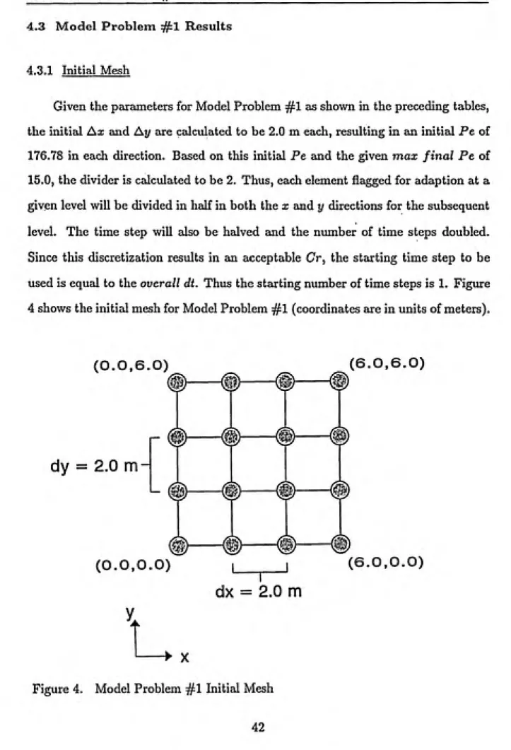
4.3 Model Problem #1 Results... 42

4.3.1 Initial Mesh... 42

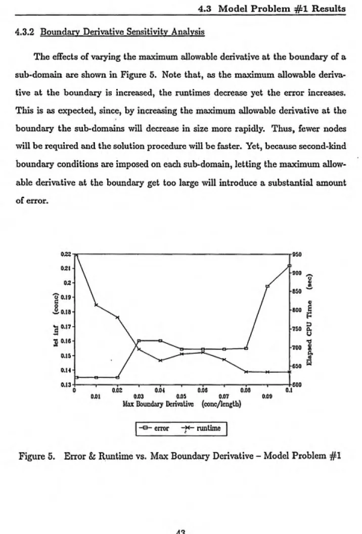
4.3.2 Boundary Derivative Sensitivity Analysis ... 43

4.3.3 Multi-Level Solution Procedure... 44

4.3.4 Error Analysis... 59

4.3.5 Adaptive/Non-Adaptive Comparison... 62

4.4 Model Problem #2 Results... 67

4.4.1 Initial Mesh... 67

4.4.2 Multi-Level Solution Procedure... 69

4.4.3 Error Analysis... 69

4.4.4 Adaptive/Non-Adaptive Comparison... 73

5 Conclusions and Recommendations... 78

5.1 Conclusions... 78

5.2 Recommendations... 79

6 Appendices... 81

6.1 Appendix A: The Finite Element Method - General... 81

1 Sample Initial Mesh... 32

2 Sajnple Refinements... 34

3 Simulation Flowchart... 36

4 Model Problem #1 Initial Mesh ... 42

5 Error & Runtime vs. Max Boundary Derivative - Model Problem #1 .... 43

6 Multi-Level Grid - Model Problem #1, Time Step 1... 45

7 Model Problem #1 Results: Time Step 1 - Levels 1 & 2... 47

8 Model Problem #1 Results: Time Step 1 - Levels 3 & 4... 48

9 Model Problem #1 Results: Time Step 1 - Level 5 k Non-Adaptive... 49

10 Model Problem #1 Results: Time Step 2 - Levels 1 & 2... 50

11 Model Problem #1 Results: Time Step 2 - Levels 3 & 4... 51

12 Model Problem #1 Results: Time Step 2 - Level 5 & Non-Adaptive... 52

13 Model Problem #1 Results: Time Step 3 - Levels 1 & 2... 53

14 Model Problem #1 Results: Time Step 3 - Levels 3 & 4... 54

15 Model Problem #1 Results: Time Step 3 - Level 5 k Non-Adaptive... 55

16 Model Problem #1 Results: Time Step 4 - Levels 1 &; 2... 56

17 Model Problem #1 Results: Time Step 4 - Levels 3 & 4 . ... 57

18 Model Problem #1 Results: Time Step 4 - Level 5 k Non-Adaptive... 58

19 Resultant ||e||2 Error - Model Problem #1... 60

20 Resultant ||e||oo Error - Model Problem #1... 61

21 Adaptive/Non-Adaptive ||e||2 Comparison - Model Problem #1... 63

22 Adaptive/Non-Adaptive ||e||oo Comparison - Model Problem #1... 64

23 Adaptive vs. Non-Adaptive Storage Requirements - Model Problem jfl . . . 65

24 Adaptive vs. Non-Adaptive Rtmtimes - Model Problem ^1 ... 67

26 Resultant ||e||2 Error - Model Problem #2... 71

27 Resultant \\e\\^ Error - Model Problem #2 ... 72

28 Adaptive/Non-Adaptive |le||2 Comparison - Model Problem #2... 74

29 Adaptive/Non-Adaptive ||e||oo Comparison - Model Problem #2... 74

30 Adaptive vs. Non-Adaptive Storage Requirements - Model Problem ^2 ... 76

31 Adaptive vs. Non-Adaptive Runtimes - Model Problem ^2... 77

1 Physical Properties - Model Problems 1 & 2... 39

2 Simulation Parameters - Model Problems 1 & 2 ... 41

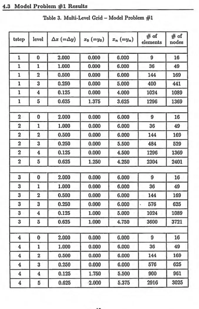
3 Multi-Level Grid - Model Problem #1... 46

4 Resultant ||el|2 Error - Model Problem #1... 60

5 Resultant ||e||oo Error - Model Problem #1 ... 61

6 Adaptive vs. Non-Adaptive Error - Model Problem #1... 62

7 Adaptive vs. Non-Adaptive Storage Requirements - Model Problem #1 . . . 65

8 Adaptive vs. Non-Adaptive Runtimes - Model Problem #1 ... 66

9 Multi-Level Grid - Model Problem #2... 70

10 Resultant ||e||2 Error - Model Problem #2... 71

11 Resultant ||e||oo Error - Model Problem #2 ... 72

12 Adaptive vs. Non-Adaptive Error - Model Problem #2... 73

13 Adaptive vs. Non-Adaptive Storage Requirements - Model Problem ^2 ... 75

1 Introduction

1.1 Purpose and Scope

All water beneath the land surface is referred to as groundwater. The equivalent

term for water on the land surface is surface water. Groundwater occurs in two

different zones. One zone, which occurs immediately below the land surface in most areas, contains both water and air and is referred to as the unsaturated zone. The unsaturated zone is almost invariably underlain by a zone in which all interconnected openings are full of water. This zone is referred to as the saturated zone. Water

in the saturated zone is the only groundwater that is available to supply wells and springs. More than half of the total U. S. population depends on groundwater for

their drinking water supply (Conservation Foundation, 1985). This includes a large

majority of rural residents as well as areas of very large population concentrations such as Long Island and Miami. Thus, the study of groundwater quality is very important not only in terms of environmental protection but also as it applies to

public health and safety concerns.

From the standpoint of groundwater occurrence, all rocks underlying the Earth's surface are classified either as aquifers or confining beds. An aquifer is a rock unit that will yield water in a usable quantity to a well or spring. (In geological us¬ age, "rock" includes unconsolidated sediments.) A confining bed is a rock unit

that restricts the movement of groundwater either into or out of adjacent aquifers

(Heath, 1980). Through either natural or "man-made" processes, many types of contaminants may enter an aquifer and, upon doing so, pose an immediate and/or

long-term threat to human health and the environment. For example, gasohne or other petroleum products may enter soils and groundwater from leaking under¬

groundwater system through agricultural runoff and subsurface drainage. Toxic chemicals may leach out of hazardous chemical storage facilities or hazardous waste landfills and enter the groundwater. Contaminants may also enter a groundwater system through leachate from solid waste landfills. Contamination of aquifers is becoming a major environmental and public health problem, particularly in light of the difficulty involved in attempting to clean-up a contaminated aquifer. Re¬ cent efforts at cleaning-up contaminated aquifers have been less than satisfactory

in achieving their desired results.

In order to adequately assess the implications of groundwater contamination

and recommend a remediation approach, some type of estimate as to the fate and

transport of the contaminant(s) within the groundwater system is necessary. This

is a difficult task, however, due to the complexity of the physical, chemical and biological processes occurring within the subsurface environment. The intrinsic

heterogeneity of porous media present in most groundwater systems complicates the

physics of the groundwater flow, while the possible interaction of many chemical

processes complicates the prediction of the fate of the contaminants.

A particularly valuable tool in estimating the fate and transport of contam¬

inants within an aquifer is mathematical modelling. The fate and transport of

contaminants can be represented in terms of mathematical (governing) equations

derived from the actual physical, chemical and biological processes occurring within

the groundwater system (to the best of our knowledge). These equations then con¬

stitute a mathematical model of what is occurring in the underlying process. This is not an exact model, however, since it is dependent upon the assumptions and

empiricism involved in the derivation of the governing equations.

For contaminant transport problems, the governing equations usually assume

the form of partial differential equations or sets of partial differential equations

1.1 Purpose and Scope

characteristics, boundary conditions, and initial conditions, these equations can be

solved analytically or approximated numerically. The solutions axe then used to estimate the concentration of the contaminant(s) at any given time and location within the domain in question. For many cases, analytical solutions are sufficient

to provide the range of sophistication needed. However, more complex transport problems transcend the available analytical solutions and must be approximated numerically. Even for these more complex problems, analytical solutions axe im¬ portant for preliminary analysis and should also be used to aid in the validation of

the numerical approximation.

In the area of modelling of groundwater systems, many numerical methods have

been shown to accurately approximate solutions to the governing flow equations or

many of these methods fail to remain accurate over all possible conditions and domains. An example of the failure of these numerical methods to accurately reflect the underlying physical process is the so-called sharp-front problem in the transport of a contaminant through a groundwater system. The term "sharp-front" refers to the propagation of a well-defined concentration front through a given domain. These

sharp fronts arise in cases of advective-dominated groundwater flow and for certain biological conditions occurring within the groundwater system.

1.2 Research Objectives

The objectives of this research are to investigate methods used to captture

sharp fronts and to develop a numerical method that will accurately and efficiently

remediation schemes for contaminated aquifers, and to design safe land disposal of

2 Background

2.1 Hydrodynamics

After a contaminant has entered a groundwater system, several mechanisms are

responsible for the migration of the contaminant away from its source. The

ground-water flow field governs the direction and velocity of a contaminant. This process

— the transport of contaminants resulting from the bulk motion (mean rate) of the

groundwater — is referred to as advection. Groundwater velocities in aquifers made

up of sand and gravel typically range between 1 meter/year (m/y) and 1,000 m/y.

In most cases, the flow velocities under natural hydraulic gradient conditions are

probably between 10 m/y and 100 m/y. In the zone of influence of a high-capacity

well, however, the artificially increased gradient substantially increases the local

velocity (Mackay et al., 1985). The lack of agreement between the observed trans¬

port of a conservative (non-reactive, non-decaying) contaminant compared to the

expected migrations due to advection alone is a result of hydrodynamic dispersion.

Hydrodynamic dispersion tends to spread a contaminant in both the longitudinal

(i.e., in the direction of flow) and the transverse directions. It is a dilution process

that occurs as a result of spatial variation in aquifer permeability, fluid mixing, and

molecular diffusion (Roberts et al., 1982). Hydrodynamic dispersion is equal to the

sum of mechanical dispersion and molecular diffusion.

Mechanical dispersion is caused by several phenomena, the first of which can

be explained by looking at the microscopic velocity distribution (velocity profile)

of a fluid flowing through porous media. Because of the effects of friction at the

solid(grain)/fluid interface, a drag force will be imparted on the fluid flowing through

the media. This drag force will increase as the grain surface is approached, thereby

from the solid/fluid interface approaches zero). Midway between grains, the effects

of friction are minimized and the fluid velocity is largest. This variation in drag

forces causes a deviation from mean flow and leads to a distribution of velocities

within the pores. Another cause of mechanical dispersion is the differences in the

size of the openings through which the fluid is flowing and the texture of the soil grains within a porous media. These differences lead to variations in velocities within a porous media, even neglecting the velocity distribution that exists within a single pore opening. This is considered a microscopic phenomenon, but is at a

scale that is somewhat larger than the single pore velocity dispersion phenomenon.

At a slightly larger — but still microscopic — scale, it is found that adjacent pore openings are not continuous. This causes the fluid to follow a circuitous route through the media rather than a direct route as in the case of fluid flowing through

a pipe, for example. This complex flow pattern results in a distribution of total

distances traveled at the microscopic scale to travel an equivalent unit distance in

a macroscopic reference system. If all other processes are incidental, this process

yields a distribution of velocities in the longitudinal direction and spreading of the

contaminant in the transverse directions.

Mechanical dispersion processes are not the only microscopic processes that

lead to dispersion in a porous media. If they were, a contaminant slug in a stagnant

flow field would not disperse, which we know is not the case. The phenomenon that causes such dispersion is Brownian motion and the result of this random motion is

the process of molecular diffusion. The mass flux of a solute from a region of high

concentration to a region of lower concentration resulting from molecular diffusion

is described by Pick's flrst law. Molecvilar diffusion is important only for regions of

low velocity.

2.1 Hydrodynamics

contaminant at a given location significantly earlier than the arrival time that is ex¬ pected solely on the basis of the average groundwater flow rate. In field and column studies, the dispersion parameter must be determined by tracer experiments.

2.2 Advective-Dispersive-Reactive Equation

The advective-dispersive-reactive (ADR) equation is the foundation of simu¬ lating siibsurface transport of solutes. The ADR equation can be generally written

as (Bear, 1979):

^ = V.(D,.VC)-vVC+(^) +r(C) (1)

where C is the concentration of the solute, t is time, T>h is the hydrodynamic

dispersion tensor that includes the effects of mechanical dispersion and molecular

diffusion, v is the mean pore velocity vector, [dC / dt) rxn is a rate of change

degradations, and T{C) is an internal source or sink term.

In the absence of internal sources or sinks, the equation can be simplified to

f = V.(D..VC)-v.VC+(§) (2)

For the case of two-dimensional flow, where advection and dispersion occur in the

X and y directions, the equation becomes

dC ^ d'^C „ d'^C ^ d^C „ d'^C dC dC ^^

2.3 Numerical Methods for Solving the ADR Equation

The ability to acctirately approximate the solution to the ADR equation is the

cornerstone for a successful simulation of solute transport, regardless of whether a deterministic or stochastic approach is used. Many numerical methods have been employed to solve the ADR equation. Most numerical methods can be classified into three major categories: Eulerian, Lagrangian, and mixed Lagrangian-Eulerian approaches (Neuman, 1984). In the Eulerian approach, the equation is discretized by a grid system fixed in space. The finite difference, finite element, collocation, and boundary integral methods are examples of the Eulerian approax:h. In the La¬ grangian approach, either a deforming grid or a fixed grid in deforming coordinates can be used. Particle-tracking methods are examples of the Lagrangian approach. In the mixed Lagrangian-Eulerian approach, a fixed grid is used but with two steps of computations: the first step is to compute the Lagrangian concentrations with particle-tracking methods, and the second step is to compute the final concentration with one of the Eulerian methods (Yeh, 1990).

Experiments have shown that the Eulerian approach using Galerkin finite el¬ ement methods (FEM's), point-collocation FEM's, or finite difference methods

(FDM's) have performed well for dispersion/diffusion dominant transport prob¬

lems. FEM's are widely used in the solution to the groundwater transport equations because of their ability to describe geometrically complex domains. For advective-dominant transport problems, oscillating approximating solutions may result when the Eulerian approach is used in conjunction with FDM's or FEM's. These os¬ cillations are a result of an inadequate discretization in space and/or time. The

two dimensionless numbers that are often used to characterize the discretization in

2.3 Numerical Methods for Solving the ADR Equation

Pe=!^ (4)

and the Courant number, Cr, which is given by

Cr = ^ (5)

The easiest way to eliminate numerical oscillations is to restrict the spatial grid

size. An alternative is to use upwind FDM's (Chaudhari, 1971; Lantz, 1971; Todd

et al., 1972; Bresler, 1973; Chaudhari, 1973; van Genuchten and Wierenga, 1974; Laumbach, 1975; Book et al., 1975; Holly and Preissman, 1977; van Genuchten and Gray, 1978; Ciment et al., 1978; Leventhal, 1980; Lasseter and Karalcas, 1982; Larson, 1982a, 1982b) or upstream FEM's (Huyakorn, 1976; Lapidus and Finder, 1982; Westerink and Shea, 1989; Cantekin and Westerink, 1990) that are able to

eliminate oscillations for 0 < Pe < oo and Cr < 1 (Jensen and Finlayson, 1980). The Lagrangian approach can help avoid the problem of oscillations (Vaxoglou

and Finn, 1982; Botha et al., 1982; O'Neill, 1986), but it has several severe draw¬ backs. First, for a long-term simulation, excessive deformation of the grid system will result, which unfortunately is prone to numerical instability (Yeh and Chou, 1981). Second, when the region of interest is composed of multimedia, the deformed grid may cross the material boundaries, which may cause difficulties in the handling of equation parameters, especially if sorption and chemical reactions are important. Third, when multiple sources are encountered, concentration fronts may propagate in different directions and cross each other at various angles, which would result in mesh tangling so that the simulation is stymied (Yeh, 1990).

the method of characteristics, uses a Lagrangian approach in dealing with the ad¬ vection terms and an Eulerian approach for all other terms in the equation. In the Lagrangian step, particles are released into the domain, each representing a certain concentration, and moved according to the mean rate of groundwater flow

(advection). By tracking these particles within the domain, the concentrations at

each nodal location due to advection alone can then be approximated by taking the average of the concentrations of the particles present at that location. A FDM or FEM is then applied to the dispersive-reactive PDE to approximate the final

concentrations resulting from the additional effects of dispersion/diffusion and re¬

actions. Each particle present at a certain nodal location is then given the value of the concentration at that node, and the process is repeated for as many time

steps as desired. Either continuous forward particle tracking (CFPT) (Konikow

and Bredehoeft, 1978), single-step reverse particle tracking (SRPT) (Molz et al.,

1986), or a combination of both (Neuman, 1984) can be used. The SRPT may in¬

troduce a significant amount of numerical dispersion (Yeh and Tripathi, 1987). For

straightforward, and the constant handling of a large number of particles is trou¬

blesome and time consuming. The combined SRPT and CFPT approach eliminates

some of these deficiencies (Neuman, 1983). Since the solution quality depends on

reduced compared with using CFPT alone (Yeh, 1990). This numerical method

used to solve first-order linear PDE's (and second-order linear hyperbolic PDE's

that can be reduced to a system of first order linear PDE's) based on the geometric

2.3 Numerical Methods for Solving the APR Equation characteristics would be very effective in approximating the solution to the ADR equation in the case of advective-dominant flow. Although this method is effective and rather simple, it poses quite a few problems. First, accurate bookkeeping of a large number of particles is necessary, giving their coordinates and concentration. Second, the method introduces some numerical dispersion when the concentrations

are calculated from the number of particles. Third, there may be a net loss of

solute at the front of the system in a mesh where dispersion introduces solute but where there are no particles. This can be corrected by introducing new particles, but this makes the method even more complex. Fourth, the method does not con¬ verge systematically when the number of particles is increased (Marsily, 1986). The practical difficulties associated with the utilization of the method of characteristics are evident to anyone who attempts to simulate a field situation. The programming sophistication required to generate an efficient yet generally acceptable code is con¬ siderable. Moreover, the method does not have the same degree of mathematical

rigor as that identified with other solution procedures (Huyakorn and Pinder, 1983).

of the DPRW are that it does not involve numerical dispersion since concentra¬ tions are never calculated. It also conserves mass and, moreover, it is possible to take into account reactions during transport, e.g., radioactive decay: the mass of

each particle is simply decreased as a function of time. The difficulties are due to the large number of particles and their bookkeeping, particularly when the velocity

varies a great deal in the medium. Also, the DPRW is unstable when the number of

particles is increased; i.e., the solution oscillates and must be smoothed. Therefore it is often not very accurate (Marsily, 1986). In fact, the convergence of the solution

is a function of y^n^, where Up is the total number of particles, making accurate

solutions costly.

From the above discussion, it is clear that the Eulerian approach (particu¬ larly the FEM due to its ability to describe geometrically complex domains) is still

the simplest and most straightforward way to solve advective-dispersive problems, provided that numerical oscillations, phase errors, numerical dispersion, and damp¬ ening can be eliminated. The easiest way to eliminate these errors is to restrict the spatial grid size such that the mesh Peclet number is less than a certain crit¬

ical number which depends on the numerical scheme used (Jensen and Finlayson, 1980). Using a fine-grid system throughout the entire domain may not be practical for many problems, particularly for large-scale simulations. Since oscillations in the

approximating solution tend to occur in regions where steep gradients of concentra¬

________ 2.3 Numerical Methods for Solving the APR Equation

critical value. A true adaptive procedtire must be based on some type of error esti¬ mator so that the overall error is guaranteed to diminish throughout the course of

a simulation.

Before an adaptive FEM can be formulated, a complete understanding of the

standard Bubnov-Galerkin FEM and the recent developments in the axea of adap¬ tive FEM's, including error estimation and re-meshing schemes, is necessary. The following discussions provide a background in these areas.

2.4 The Finite Element Method

The finite element analysis of a physical problem czin be described as follows

(Huyakorn and Pinder, 1983):

(1) The physical system is subdivided into a series of finite elements that axe

connected at a discrete number of nodal points; this process is often called

"discretization."

(2) A matrix expression is developed to relate the nodal variables of each

element. The resulting matrix is commonly referred to as an "element matrix." For a discrete problem, the element matrix relation can often

be established via direct physical reasoning. For a continuum problem, the element matrix expression must be obtained via a more general math¬ ematical formulation that generally makes use of either a variational or

weighted residual method.

(3) The element matrices are combined or assembled to form a set of algebraic

equations that describes the entire global system. The assembly procedure

is performed in such a way that certain compatibility conditions are satis¬ fied at each node shared by different elements.

(4) Prescribed boundary conditions are incorporated into the assembled or

(5) The resulting set of simultaneous algebraic equations is solved. Here,

many different solution algorithms can be employed, including Gaussian elimination, Choleski decomposition, iterative techniques such as the SOR method, and steepest descent algorithms such as the conjugate gradient

method.

The formulation of the element matrix equations for continuum problems (as op¬ posed to discrete problems) can be accomplished via the use of either a variational

or a weighted residual approach. Early applications of the FEM were formulated

using the variational approach. However, the so-called Galerkin weighted residual

approach gained popularity because of its generality in application, particularly to non-self-adjoint problems, which cannot be cast in variational form.

Various classical weighted residual methods can be generated, depending on the choice of the weighting functions. Examples of these methods include: the point collocation method in which the weighting functions are chosen to be Dirac delta

functions, thus making the integration and assembly of the global coefficient matrix

much simpler (this malies these methods more attractive for non-linear ADR prob¬

lems where the coefficient matrix will have to be formed and re-formed numerous

times); the standard Bubnov-Galerkin method in which the weighting functions are

weighting functions (Huyakorn and Pinder, 1983). (See Appendices A and B for

2.5 Convergence of the Finite Element Method

2.5 Convergence of the Finite Element Method

In finite element analysis, convergence can be achieved in several different ways.

The three basic modes of convergence are:

(1) The basis functions for each element can be fixed and the diameter of

the largest element, /imax? allowed to approach zero. This mode is called

/i-convergence.

(2) The finite element mesh can be fixed and the minimal order of (polynomial)

basis functions, p^^, allowed to approach oo. This mode is called

p-convergence.

(3) Mesh refinement can be combined with increments in the order of polyno¬

mial basis functions.

Convergence has been the basis for justification of the FEM but until recently has

not actually been attempted in the computational process.

2.6 Feedback and Adaptivity

In the application of the FEM, one of the most critical decisions is the design

of the mesh and selection of the elements. The question of whether the choice of

mesh and basis functions is adequate for the purposes of a simulation is not always

addressed directly. Rather, the analyst relies on his judgement and experience to

ensure that the mesh is sufficiently small or the polynomial orders are sufficiently

high so that the error of analysis is small (e.g., Ebner, 1975). Because the analyst's

judgement is not always reliable, there is a growing interest in feedback and adap¬

tivity. A numerical process is called a feedback process when it uses the data in a sequential way so that the flow of computation is determined by some feedback

feedback procedure is advantageous only if it has some useful properties, for ex¬ ample, if it produces the required information by less work and higher reliability

than the nonadaptive process. All the modem ODE solvers for initial value prob¬

lems and quadratures are feedback methods. Feedback methods are increasingly in the focus of interest in the area of numerical solution of PDE's and computa¬ tional mechanics. It seems that successful computation of today's large complex problems cannot be made without some kind of feedback or adaptive approach. A

feedback procedure (method) is said to be adaptive if it is optimal with respect to

a certain performance measure; hence the adaptivity is a relative notion. Adap¬

tivity is essentially comprised of two parts: (1) the determination of the sources of error in the solution and estimation of their magnitude; and (2) the improvement

of the axicuracy of approximation by changing the number or distribution, or both, of the degrees of freedom. The foundation of feedback and adaptivity is explained in Rheinboldt (1983) and surveys of adaptive procedures have been provided by

Thompson (1985) and Babuska et al. (1986). The two main difficulties associated with error estimating and adaptivity are: (1) the cost of computations associated with error estimation; and (2) the virtual impossibility of embracing a fully adaptive structtire into an existing code structure (Zienkiewicz and Zhu, 1987).

2.7 Sources of Error in the Finite Element Method

In a practical finite element analysis the major sources of error are: (1) trun¬

cation error due to the use of low degree polynomials; (2) geometric sovirces of

______________________2.7 Sources of Error in the Finite Element Method

improve upon the solution accuracy correspond to the three modes of convergence. These approaches are: (1) to selectively refine the mesh using low order elements (the /i-version of the FEM); (2) to add progressively higher-order hierarchic basis

functions while keeping the mesh constant (the p-version of the FEM); and (3) a

combination of (1) and (2) (the /i-p-version of the FEM). It is therefore essential to

be able to get a quantitative assessment of the quality of the approximate solution

and the capabilities of refinement. Thus, an integral part of a rational adaptive scheme is some means of estimating a posteriori (after one approximate solution is

obtained for an initial mesh and element family) the local approximation error.

2.8 A Posteriori Error Estimates

The classical approaches to error analysis are computationally expensive. A process for providing a simple error estimator is presented by Zienkiewicz and Zhu

(1987). Zienkiewicz and Craig (1986) explain the advantages of using a p-method

combined with a hierarchic formulation when solving elliptic PDE's. This proce¬ dure simplifies the error estimation process. It also provides for the relative ease of

obtaining fast convergence, improved equation conditioning and possibilities of iter¬

ative solutions of refinement equations (Zienkiewicz and Craig, 1986). However, the

efficiency here involves generally abandoning a standard finite element structure. Oden et al. (1989) address the issue of a posteriori error estimation for h-p FEM's as part of a general approach to the development and implementation of a h-p version of the FEM (Demkowicz et al., 1989; Oden et al., 1989; Rachowicz et

al., 1989). They experiment with five methods for elliptic boundary value problems (BVP's). These five methods are: (1) element residual methods, in which the residual in a numerical solution (the function defining the measure of how much the

local error; (2) duality methods, valid for self-adjoint elliptic problems, in which the theory of convex optimization is used to derive upper and lower bounds of the element errors; (3) subdomain-residual methods, where the local BVP for the error in a given element is formulated over a patch of elements surrounding the element; (4) interpolation methods, which use the interpolation theory of finite elements in Sobolev norms to produce rapid (and sometimes crude) estimates of the local error over individual elements; and (5) post-processing methods, where an estimate is obtained by comparing a post-processed version of the approximate solution with

the approximate solution.

Progress has been made in developing a posteriori error estimates based on the computation of residuals, and the survey of Babuska (1984) provides a detailed discussion of such approaches for a restricted class of problems. One of the main

features of these a posteriori error estimates is that they involve local, rather than

global, computations. They are given in an asymptotic form which guarantees ac¬ curacy when linked to adaptive refinement algorithms as /i —> 0, but experience has shown that they can provide information about the errors on a finite grid. The work for Unear, self-adjoint boundary value problems is now well founded (Kelly et al., 1983). Alternatively, Diaz et al. (1983) proposed an error-estimation method based

on interpolation error estimates for finite elements. This method has the advantage

that it does not require the solution of local auxiliary problems for error indicators for each element, but, among other things, it has the disadvantage of requiring the estimation of higher-order derivatives over each element and being nonlocal. Demkowicz et al. (1985) present an /i-type adaptive scheme which employs er¬ ror estimators based on interpolation estimates and extraction formulas (Babuska and Miller, 1984a, 1984b) for highly accurate estimates of second derivatives. This

2.8 A Posteriori Error Estimates

Babuska, Rheinboldt and their co-workers developed a posteriori error esti¬ mates for the bilinear element which are sufficiently robust to reliably indicate when the error is small (Babuska and Rheinboldt, 1978a, 1978b, 1979a, 1979b). Closely related to this work was the development of adaptive schemes that auto¬ matically enrich the finite element mesh on the basis of local error indicators to give convergence to near-optimal meshes and re-solve until a pre-specified accuracy is achieved. These mathematical processes lead to the question of the local as well as global interpretation of the error and the definition of optimality in the finite el¬ ement mesh, since the contribution of elements to the total error of approximation generally vaiies from element to element. Thus, a posteriori error estimates are not only important for an assessment of the reliability of the results, but also provide a

means for adaptive optimization of the finite element mesh.

2.9 Adaptive Mesh Refinement

The need to solve large two- and three-dimensional boundary-value problems efficiently and accurately has led to an increased research interest in mesh refine¬

ment strategies for finite element computations (Babuska et al., 1986). Much of the

focus of this work has been directed to the analysis of a posteriori error indicators (e.g., Babuska and Rheinboldt, 1978a) and to efiicient iterative solution (e.g. Carey and Seager, 1985). For remeshing, two aspects are important. An adequate mea¬ sure must be introduced to decide whether remeshing is required and the logic for

automatic remeshing must be determined for practical applications.

spacing is small only in regions where the solution exhibits sharp fronts needing fine-scale spatial resolution. Since the sharp fronts move, it is necessary to refine the grid

adaptively, so that the refined zone follows the front. Since this drastically increases

the problem size and cost (particularly in the case of two- or three-dimensional

domains), user-defined selective refinement in areas of sharp velocity or pressure

gradients is commonly used for large scale simulations (Dannelongue and Tanguy, 1990). This requires however some a priori knowledge of the solution. As this is

not generally the case, adaptive techniques that automatically determine the areas

of insufficient accuracy and refine the mesh accordingly are viewed as one of the

promising solutions for the reduction of computational cost.

Recently, much progress has been made with the introduction of numerical grid generation methods that control the mesh size and allow the nodes of the grid to move smoothly with the critical regions that require their presence. In the numerical analysis literature some criteria of grid generation used are: the con¬

centration of the nodes in the regions with high gradients (Dwyer and Sanders, 1978; Larouturou, 1985), Lagrangian approaches where the nodes are moved at mean fluid velocity or at some other characteristic velocity in the fluid (Ramos, 1983), and moving Galerkin finite elements (Miller and Miller, 1981; Miller, 1981). Oliveira and Oliveira (1988), in considering finite difference discretizations of trans¬

port equations and advective-diffusive equations, proved that if the mesh density is proportional to the spatial gradient and the nodes are moved at the advection speed, then the spatial truncation error is minimized. Thus the "optimal grid" has the same characteristics as the physical problem: the density of the grid corresponds

to the spatial gradient and the speed of the grid corresponds to the advection speed.

2.9 Adaptive Mesh Refinement

approximate solution. The approximate problem on the new mesh is then solved and

the refinement step is repeated. The successive solution and refinement calculations

axe repeated until a satisfactory solution is achieved. Dannelongue and Tanguy

(1990) found that, for a given error level, an iterative sequence of meshes will be

more economical than a single remeshing.

Much effort has been put into the determination of optimal meshes in the sense that the error is minimized for a given number of degrees of freedom (Turcke and Mc-Neice, 1972; Carroll and Barker, 1973; Babuska, Rheinboldt and Mesztenyi, 1975; Melosh and KiUian, 1976; Sewell, 1976; Babuska, 1976; FeUppa, 1977, 1978). With the cost of this optimization being prohibitive, general guidelines, frequently used in practice, were established to obtain efficient meshes (Oliveira, 1971; Tvucke and McNiece, 1974; Turcke, 1976; Melosh and Killian, 1976; Melosh and Marcal, 1977; Melosh, 1980; Shepard, 1980; Shepard et al., 1980). Starting from an arbitrarily defined mesh, several questions can immediately be raised. At one extreme a suffi¬

ciently refined mesh can be presented such that the error tolerance is immediately

satisfied and no further refinement is needed. At the other, a very crude mesh can be used as a starting point and a large number of iterations be necessary to achieve the pre-specified error tolerance. The path to follow will obviously depend on the computational costs. Another question can be raised in relation to the number of degrees of freedom introduced at each step. The final choice has to be a function of the cost since the more restrictive the method is, the more solution steps will be necessary to achieve a given accuracy. The important fact is that a process of this nature followed by evaluation of the error at each stage will lead to an arbitrar¬

ily reduced error (apart from computer limitations). The process will be stopped

(Babuska and Rheinboldt, 1979b). Error estimates showing the dependence of the rate of convergence on the mesh size are well-known (Ciarlet, 1978).

An important observation is that the finite element solution on a given coarse

mesh provides an appropriate initial guess for iterative solution on the next (re¬ fined) mesh. Accordingly, the simplest strategy is to use the finite element solution

and interpolate the finite element basis to produce an initial vector for iterative

solution on the new mesh. It has been observed that, even though the finite ele¬

ment interpolant provides a good estimate of the solution on the next mesh, the iterative method is still not as fast as desired. This is particularly true for problems with steep local gradients and layer zones since the coarse mesh solution provides a poor starting iterate for the refined problem in these regions. Carey and Seager

(1985) examined alternative approximation techniques to improve the starting iter¬ ate and accelerate convergence. These techniques involve the introduction of local

elliptic projections to provide improved local approximations to the finite element solution of boimdary-value problems. This approach yields a composite global ap¬ proximation that is more accurate and provides a good starting value for iterative

solutions.

Allen and Curran (1989) present an adaptive local grid refinement scheme for use in finite element collocation models for highly advective fluid flows. Of special

interest in this scheme are the algorithmic aspects of the procedure, which is readily amenable to implementation on parallel-architecture computers.

A series of articles by Brackbill and Saltzman (Brackbill, 1982; Saltzman and Brackbill, 1982; Brackbill and Saltzman, 1982) presents a generalization of the

conformal-map technique, which couples mesh generation in an intuitive way with

the resolution of the approximate problem. This method lacks precise mathematical

2.9 Adaptive Mesh Refinement

objection faced by the Diaz method is that the functional being minimized supplies

us only with a very rough estimate of the interpolation error, which was, even then, developed only for the purpose of an a priori error estimate. In other words, all the information about the dependence of the interpolation error upon the mesh geometry is stored only in a maximal size of a current element (parameter h) which is very imprecise information. Demkowicz and Oden (1986) attempt to couple both of these methods. In minimizing the interpolation error, they do not attempt to determine an optimal mesh. Rather, they are interested in suboptimal meshes that result in a better FE approximation, not necessarily the optimal one. Thus, their method is a generalization of the mesh generation technique.

Kikuchi (1986) develops a theory of adaptive finite element grid-design methods for finite element approximations, which can assure that the approximated solution to a given problem meets some pre-specified level of accuracy. In this approach, numerical grid-generation methods are coupled with adaptive finite elements in order to design a better finite element grid, in the sense that it reflects the solution characteristics, and to improve the accuracy of the finite element approximations

at the same time.

Although much of the focus of the work in mesh refinement strategies in FEM computations has been directed to the analysis of a posteriori error indicators and to efficient iterative solution, an important aspect is the actual refinement scheme and the data structure that supports it. These issues strongly influence the prac¬ tical feasibility of adaptive refinement, code complexity, storage "overhead" and

related considerations (Carey et al, 1988). There have been several studies of spe¬

bricks in three dimensions. Both linear (bilinear) and quadratic element types axe developed. The refinement scheme is self-adaptive and proceeds automatically to subdivide the mesh locally and yield a graded unstructured grid.

2.10 Adaptive Finite Element Methods

An adaptive FEM can be schematically described as a feedback process where the automatic construction of a quasi-optimum mesh (with respect to the involved

number of degrees of freedom) is performed in the course of the computations. In

this context, the selective and local refinement of the mesh throughout the compu¬ tations arises as a natural and desirable feature, which has induced a change in the rather static classical grid generation approach, whose main goal was the construc¬

tion of a fixed discretization of the geometry with any desired resolution (Rivara, 1989). The objective of an adaptive FEM is to control the discretization error by

increasing the number of degrees of freedom in regions where the previous finite element model is not adequate and to achieve the specified accuracy, proceeding in a most economic manner. The most efficient error reduction technique is that for which the path on the error reduction versus cost is the steepest.

Significant advancements have been made on the theory and computational algorithms for the development of adaptive strategies in the FEM in recent years. Mathematical work by Babuska and his co-workers (Babuska and Dorr, 1981; Gui and Babuska, 1986; Guo and Babuska, 1986; Babuska and Quo, 1988) shows that,

in h-p refinement, it is possible to achieve an exponential rate of convergence to

the exact solution for all problems, even those with corner singularities. The p-version also shows a higher convergence rate than the /i-p-version (Babuska, Szabo and Katz, 1981) and its implementation in different adaptive analysis strategies has

been presented by different authors (Zlenkiewicz et al., 1983; Kelly et al,, 1983;

2.10 Adaptive Finite Element Methods

Szabo, 1986b). However, the practical implementation of the optimal h-p strategy is

difficult. The reason for this is the meshing requirement and high p degrees needed,

as indicated by the analysis (Gui and Babuska, 1986; Guo and Babuska, 1986).

Zienkiewicz et al. (1989) present an effective and practical /i-p-adaptive FEM in

2.11 Applications of Adaptive Methods

Several methods have been developed that are very effective in approximat¬

ing solutions to elliptic PDE's. Adaptive multigrid methods have been proposed

by Brandt (1977). Adaptive FEM's have been developed by Babuska and

Rhein-boldt (1978b), Bank (1981), and Bank and Sherman (1981). These methods are

not as effective when applied to the time-dependent cases, or parabolic and hyper¬

bolic PDE's. Gannon (1980), Sherman and Seager (1981), and Davis and Flaherty

(1982) concentrated on parabohc and hyperbolic PDE's in developing their adap¬

tive FEM's. Miller and Miller (1981) derived moving FEM's, which they appHed to

both hyperboHc and parabolic PDE's.

Adaptive grid methods for hyperbolic equations in one space dimension have

also been considered (Harten and Hyman, 1983). Gropp (1980) and Berger and

Oliger (1984) considered local refinement finite difference methods for solving

one-and two-dimensional hyperbolic problems, one-and Flaherty one-and Moore (1985) de¬

veloped a local refinement finite element procedure for solving one-dimensional parabolic problems. In each case, uniform, fine, space-time meshes were recur¬ sively added to coarser ones tintil either an estimate of the discretization error was

boundaries of the finer grids are defined using interpolation procedures applied to

Gannon (1980), Bieterman and Babuska (1982a, 1982b), and Adjerid and Fla¬

herty (1986a, 1986b, 1986c) developed adaptive method of lines procedures for

parabolic problems that locally added and deleted finite elements in space while

performing a global refinement in time. Adjerid and Flaherty (1986a, 1986b) fur¬

ther added mesh motion to their one-dimensional procedures. The methods of

Gannon (1980) and Adjerid and Flaherty (1986c) are applicable to two-dimensional

problems on stationary meshes and axe similar in many respects to those of Babuska,

Miller and Vogelius (1983) and Bank et al. (1986) for elliptic problems.

Arney and Flaherty (1989) developed an adaptive local mesh refinement method

for time-dependent PDE's (hyperbolic and parabolic) that identifies and groups re¬

gions having larger local error indicators into rectangular clusters. The time step

and computational cells within clustered rectangles are recursively divided until a

prescribed tolerance is satisfied. The refined meshes are properly nested within

coarser mesh boundaries, thus simplifying the prescription of interface conditions

3 Model Formulation

3.1 Motivation

The goal of this research is to develop an adaptive FEM in two spatial dimen¬ sions that will provide accurate approximations to sharp-front problems. The prob¬ lem of solute transport in grovindwater systems in two spatial dimensions arises from the case where a contaminant is released from a line source; i.e, a fully-penetrating well. The release may be instantaneous, resulting in a slug source; or it may be such that a constant concentration is maintained at the point of release, resulting

in a step source.

3.2 Adaptive Mesh Refinement

This method will incorporate a multi-level, adaptive re-meshing scheme based

on a simple error estimator. The re-meshing will allow for solutions to be approxi¬

mated over a series of successively smaller domains (levels) within a given time step. These successively smaller domains will "zoom-in" on the sharp front and therefore provide a more accurate approximating solution without having to use a fine-grid system throughout the entire domain.

Yeh (1988) used a very effective zooming procedure in the "Zoomable and Adaptable Hidden Fine-Mesh Approach" (ZAHMFA) in one spatial dimension, in

which a region of the domain (which could be as small as a single element) is more

finely discretized and is treated as a hidden fine mesh. After a partial reduction of

the hidden fine-mesh system of equations, it is possible to substitute this information

back into the global system of equations and arrive at an updated approximating

does not easily extend to two spatial dimensions, due to the occiirrence of irregular nodes at the adapted region/non-adapted region interface (see Figure 1).

An alternative is to use a multi-level, adaptive procedure. One such approach is based on the convergence of the approximating solution at each node within the domain. This method, in essence, re-formulates the problem at each level, where the boundary conditions can be found from the lower levels' convergent nodes and the initial conditions can be found from the information at the previous time step. The adaption process is automatic, i.e., it does not require any input as to where a sharp front may be located within the domain a priori, or before any computations axe made. The self-adaptive procedure will automatically zoom-in on any region that requires additional discretization in order to reduce the overall error.

3.3 Error Estimation and Convergence

3.3 Error Estimation and Convergence

storage requirements substantially. Another problem with this approach is that it is

not possible to specify exactly the boundary conditions. That is, since the number of time steps is being doubled for each new sub-domain, there is no means of assigning accurate first-kind boundary conditions at each time step. This is because previous level values for convergent nodes exist only for every other time step on the current

level. In order to assign boundary conditions, some interpolation is then necessary. As the sub-domains begin to shrink to the point where the boundary values are

significantly greater than the background concentration, the error introduced by this interpolation may become substantial. Interpolation is also required to assign values at irregular nodes lying on a boundary.

Another approach to evaluating convergence of the nodes is to use a uniform

convergence criteria as opposed to the pointwise convergence criteria previously

discussed. In this approach, the boundary conditions for the initial domain (level

0) are as specified for the original global domain. The boundaries for the

each element. If the derivative is below a certain pre-specified limit then it need not

be included in the next level's domain. Then, second-kind boundary conditions can

be imposed on each of the sub-domains. In order to determine when convergence is achieved, the L^o norm of the difference vector between successive domains can be calculated and checked to see if it is below a pre-specified limit. If so, then it can be assumed that the approximating solution has converged for the given time

step. This approach is advantageous because second-kind boundary conditions can

be imposed on all the sub-domains (natural, no-flux boundary conditions if the

derivative limit is small enough). This simplifies the coding and, if natural no-flux

boundary conditions can be used, avoids the interpolation required in imposing first-kind boundary conditions. The limitation of this approach is that the sub-domains

show, however, that this is adequate. Even when using a pointwise convergence approach, when the sub-domain shrinks down to the region of the plume, most of the error has been eliminated.

A variation of the uniform convergence approach that can be used to reduce the

storage requirements and computational cost is to establish a target Peclet number limitation initially and run the simulation until the discretization is such that this criteria is satisfied. This target Peclet number approach will be used in this model.

3.4 Simulation Procedure

Using first-derivatives across elements as an indication of error, and the target

Peclet number convergence criteria, the simulation proceeds as described in the

following sections.

3.4.1 Model Inputs

To start the simulation, inputs are required for the physical characteristics of the groundwater contaminant transport system and for the simulation parameters (see Section 4.2 for tables of the input variables used in a simulation).

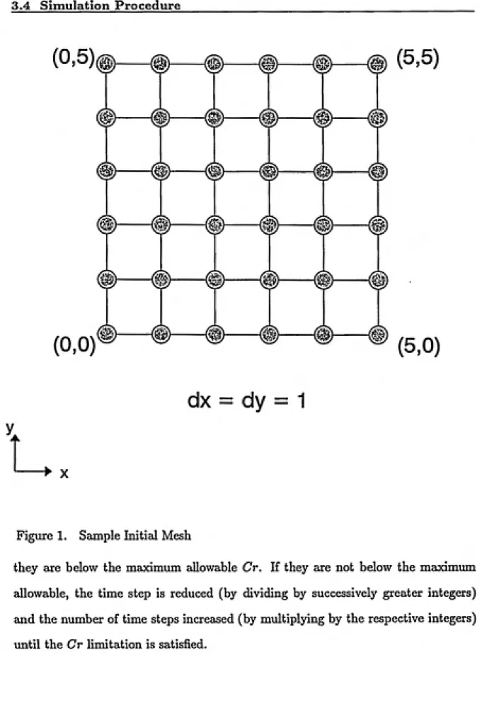
3.4.2 Initial Mesh I

At each level of the solution process, a uniform mesh is set up consisting of rectangular elements aligned with the x-y coordinate system. To determine the

initial mesh. Ax and Ay are chosen such that a node will be present where the

peak of the plume is located at the start of the simulation. This will ensure that

a non-zero value will be picked-up initially, regardless of how sharp the front is.

These Ax and Ay will also be chosen such that the maximum initial Pe limitation

is satisfied. Thus the boundaries of the domain are determined by the initial peaJc

3.4 Simulation Procedure

These variables represent the maximum x-coordinate of the left side of the domain

(vertical line), the minimum x-coordinate of the right side of the domain (vertical

line), the maximum y-coordinate of the bottom of the domain (horizontal line), and

the minimum y-coordinate of the top of the domain (horizontal line) respectively.

Once this initial discretization is established, the next step is to determine the

integer by which the elements will be divided from one level to the next. This is done by using the initial Pe, the maximum final Pe, and the total number of levels

available according to the following formula:

,. . . / initial Pe \l/nlevela-l

division > I---——;---1 (6)

\max final Pe/

The smallest integer satisfying the above expression is then used as the divider. Next, using the initial grid and the divider, a check is made to see if the Ax and Ay at any level will be less than or equal to the distance traveled by the plume

in one overall time step. If the Ax or Ay at any level will be less than the distance

traveled by the plume in one overall time step, an adjustment is made to ensure equality. If an adjustment is made, then the calculation of the divider is repeated. Adjustment of the Ax and Ay and recalculation of the divider are repeated until no

further adjustments are necessary. Once Ax and Ay are established, the boundaries

Thus an initial uniform mesh (level 0) is now in place, consisting of rectangles aligned with the x-y coordinate system. An example of such a mesh is shown in

Figure 1.

Inputs are now required concerning the magnitude and number of time steps

to be carried out. Using the given overall At (length of time intervals for desired

output), the discretization parameters Ax and Ay, and the given velocities in the

(0.5)0—m—o

m—© (5,5)

^1

(0,0)

(5,0)

dx = dy = 1

> X

Figure 1. Sample Initial Mesh

they are below the maximum allowable Cr. If they are not below the maximum

allowable, the time step is reduced (by dividing by successively greater integers)

and the number of time steps increased (by multiplying by the respective integers)

^^fl^^*^w^l^''

3.4 Simulation Procedure

3.4.3 Multi-Level Solution Procedure

The FEM is then applied to this initial mesh using given initial values and

boundary conditions to yield an approximate solution at the initial nodes. Deriva¬

tives are then calculated in both the x and y directions between adjoining nodes.

The boundaries of the next level's domain are determined by comparing these

derivatives with the maximum allowable de;rivative. Those areas where the deriva¬

tives exceed this limitation are included in the subsequent domain. Steps are taken

in this process to ensure that the domains at every level will be rectangular. Work¬

ing with rectangular domains greatly simplifies the code, however it does sacrifice

some of the efficiency of the model in using more nodes than is absolutely necessary.

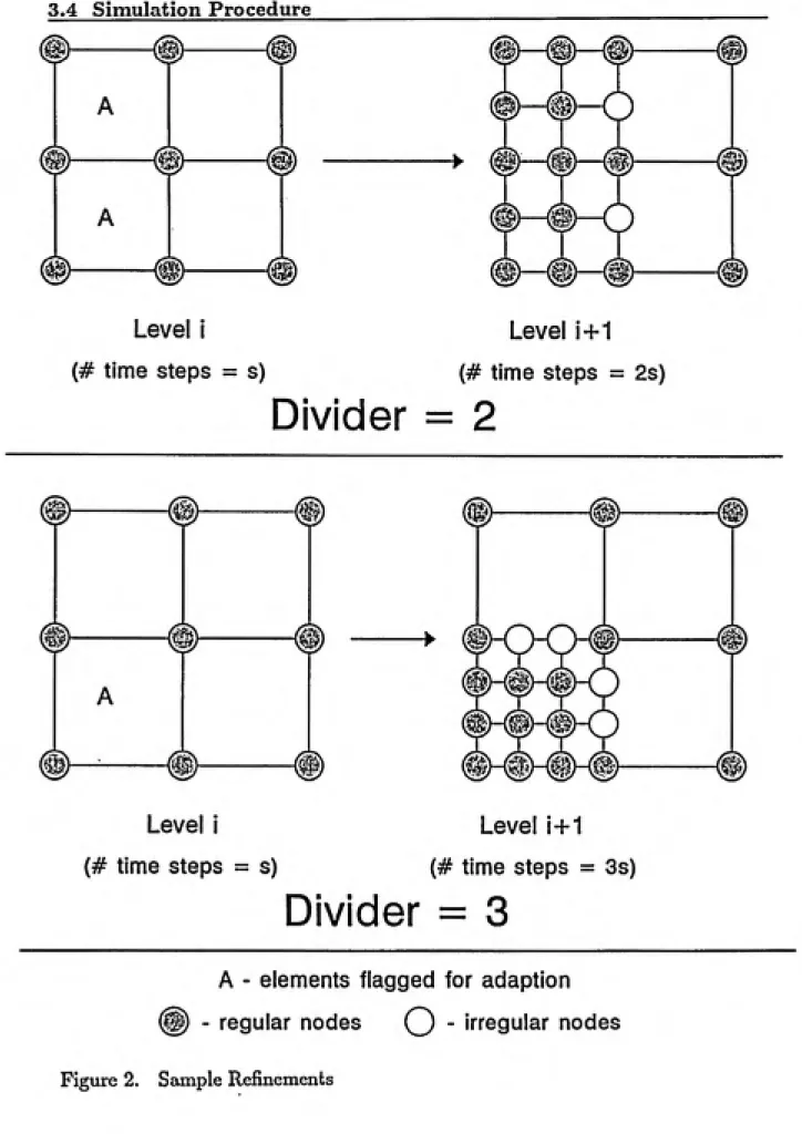
The new domain is then refined by dividing each element by the previously

calculated divider in both the x and y directions. Examples of the refinement of a

grid using a divider of 2 and a divider of 3 are shown in Figure 2. The FEM is then

carried out on this refinement (level 1) of the original mesh, again using the given

initial values but now the boundary conditions to be used are natural (second-kind,

no-flux) boundary conditions wherever the sub-domain boundary does not coincide

with a global domain boundary. Also, for this new mesh the time step is halved

and the number of time steps doubled to ensure that the Courant number remains

less than the minimum allowable — in fact it stays constant.

This refinement method will ensure that for each of the nodes in the original

mesh there will be a node in the refined mesh that assumes the same spatial location.

Because of this, it is possible to (if storage allows) compare the values obtained for

the independent variable (concentration in our case) on the original mesh to those

obtained on the refined mesh. Moreover, the convergence of the approximation on

Level I

(# time steps = s)

Level i+1

(# time steps = 2s)

Divider = 2

#

Level i

(# time steps = s)

Level i+1

(# time steps = 3s)

Divider = 3

A - elements flagged for adaption

- regular nodes Q " 'tegular nodes

3.4 Simulation Procedure

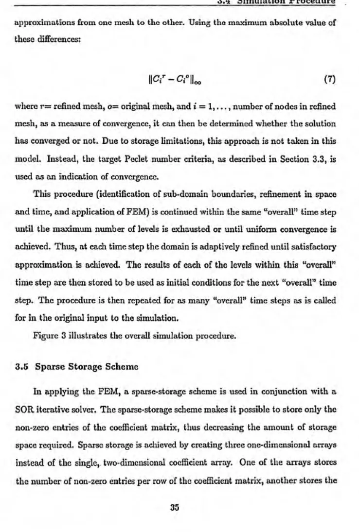
approximations from one mesh to the other. Using the maximum absolute value of

these differences:

WCi'-Ci^W^ . (7)

where r— refined mesh, o= original mesh, and i = 1,..., number of nodes in refined

mesh, as a measure of convergence, it can then be determined whether the solution

has converged or not. Due to storage limitations, this approach is not taken in this

model. Instead, the target Peclet number criteria, as described in Section 3.3, is

used as aji indication of convergence.

This procedtire (identification of sub-domain boundaries, refinement in space

and time, and application of FEM) is continued within the same "overall" time step

until the maximtmi nvimber of levels is exhausted or until uniform convergence is

achieved. Thus, at each time step the domain is adaptively refined until satisfactory

approximation is achieved. The results of each of the levels within this "overall"

time step are then stored to be used as initial conditions for the next "overall" time

step. The procedure is then repeated for as majiy "overall" time steps as is called

for in the original input to the simulation.

Figure 3 illustrates the overall simulation procedure.

3.5 Sparse Storage Scheme

In applying the FEM, a sparse-storage scheme is used in conjimction with a

SOR iterative solver. The sparse-storage scheme makes it possible to store only the

non-zero entries of the coefficient matrix, thus decreasing the amount of storage

space required. Spaxse storage is achieved by creating three one-dimensional arrays

[Parameter Input |

Determine Initial a x and Initial a y Using Peak at Initial Time & Max Initial Pe |

Determine Divider Using Initial a x,

Initial a y, Max Final Pe, and Max # Levels

Check Tliat AX, Ay Will Equal Distance Between Peaks

No Yes

Adjust Init ax, Init Ay So That ax. Ay Will Equal Distance Between Peaks Using Divider

Determine Locations of Global (Level 0) Boundaries Determine Starting a t and # Time Steps Using Max Cr

Initialize to Level 0 - Initial a x. Initial a y, Global

Boundaries, Starting a t and # Time Steps

Get Initial Values From Previous TS

Solve Using FEM (Sparse Storage SSOR) '

Determine Sub-Domain Boundaries Store Information for Level

1

Is Level >

Max # Levels? No Yes

Store_{Information for Time Step |}

Is Time Step > Max # Time Steps

No

Yes

Stop

3.5 Sparse Storage Scheme

actual non-zero values, and the third stores the column number of each of the non¬ zero entries. These three arrays contain all the information necessary to perform the SOR iterations. This provides a substantial savings in computer storage since there will be at most nine non-zero entries per row in the coefficient matrix using rectangular elements aligned with the x-y coordinate system. The coefficient matrix in this case is block-tridiagonal with each block being a tridiagonal matrix. Thus, for a large-scale simulation, the fraction of non-zero entries in the coefficient matrix

will be very small.

3.6 Storage and Memory Requirements

4.1 Analytical Solution

To validate the results of the model, the known analytical solution is compared

to the approximating solution for two "model" problems. The first model problem

is a small-scale simulation that is well-suited for graphical display of the output.

The second is a larger-scale simulation that will show more emphatically the savings

in computational cost and storage associated with the multi-level, adaptive method.

Both of the model problems are two-dimensional (line source), slug-source problems.

The analytical solution for the case of a slug source in two dimensions is given

by (Crank, 1975):

where M' is the mass of the line source per unit depth of the aquifer, n is the porosity

of the aquifer, U/,^ is the longitudinal dispersion coefficient (in the direction of the

flow), Dh^ is the transverse dispersion coefficient, Vj, is the velocity in the direction

of the mean pore velocity vector, and all other terms are as previously defined.

4.2 Model Inputs

Two types of input are required for this model. The first type will describe the

physical characteristics of the groundwater contaminant transport system. These

characteristics include the properties of the porous media and of the contaminant(s).

The second type of input specifies how the simulation will be set up and performed;

i.e., the spatial domain, the time intervals for desired results, the starting time, lim¬

4.2 Model Inputs

the FEM, the maximum number of levels to use in the multi-level procedure, and

the maximum allowable derivative at the sub-domain boundaries.

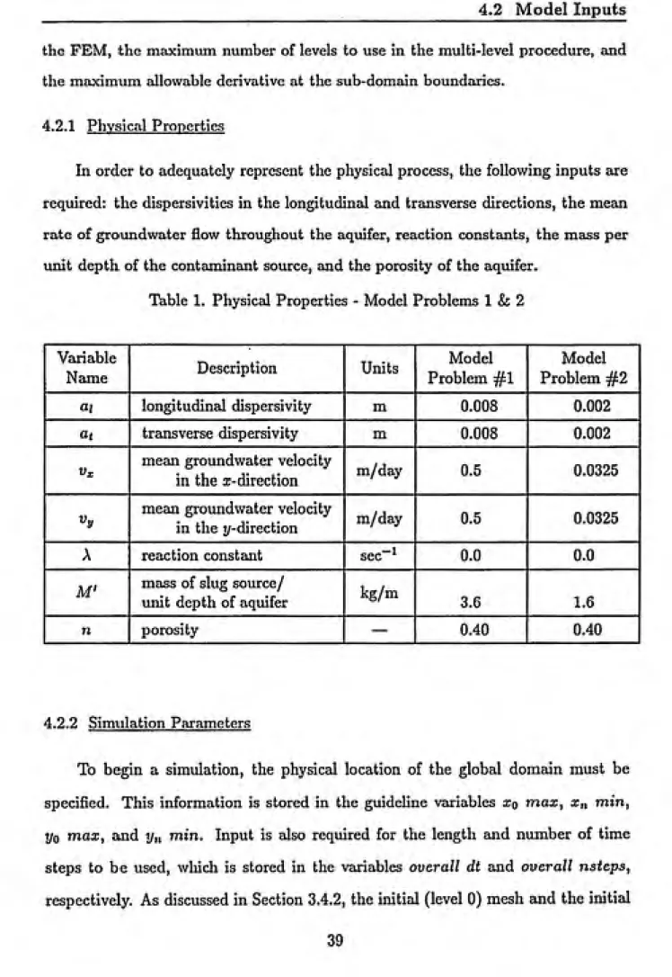
4.2.1 Physical Properties

In order to adequately represent the physical process, the following inputs cire required: the dispersivities in the longitudinal and transverse directions, the mean rate of groundwater flow throughout the aquifer, reaction constants, the mass per unit depth of the contaminant source, and the porosity of the aquifer.

Table 1. Physical Properties - Model Problems 1 & 2

Variable Name Description Units Model Problem #1 Model Problem #2

ai longitudinal dispersivity m 0.008

0.002 1

at transverse dispersivity m 0.008

0.002 1

Vx mean groundwater velocity

in the a;-direction m/day 0.5

0.0325

^y

mean groundwater velocity

in the y-direction m/day

0.5 0.0325

A reaction constant sec~^ 0.0

0.0 1

M' mass of slug source/

unit depth of aquifer kg/m 3.6

1.6 1

n _porosity 0.40

0.40 1

4.2.2 Simulation Parameters

To begin a simulation, the physical location of the global domain must be specified. This information is stored in the guideline variables xq max, x„ m.in, j/o m,ax, and y,i m,in. Input is also required for the length and number of time steps to be used, which is stored in the variables overall dt and overall nsteps,

time step to be used at each overall time step are calculated based on the limits imposed on the initial Pe and Cr numbers. These limits are input and stored in

the variables, max initial Pe and Cr^naxi respectively.

Thus, based on the given variables xq max, a:„ min, yo max, yn min, overall dt, max initial Pe, and Crmax-, ^t^ initial mesh and initial time step are calculated. The actual boundaries of the initial mesh (xq, a;„, yoj and yn) may not be the same as the guideline variables, (xq max, x„ min, t/o m,ax, and y„ min), but they will be constructed so that the initial mesh covers an area equal to or greater than that specified by the guideline variables. The initial time step that is calculated will be

less than or equal to the given overall dt.

In order to get initial values at the first time step, an input is required for the initial time variable, which represents the elapsed time from the release of the contaminant to the start of the simulation. This initial time, together with the physical location of the contaminant source, will determine the initial values at

every spatial location in the domain.

In performing the simulation, variables must be set up that will control the solution procedure and determine when the simulation should be terminated. The variables ui, 9, and max deriv are used to control the multi-level, adaptive pro¬

cedure. These variables specify how the elemental matrices are set up (implicitly

vs. explicitly), how the solution of the resulting system of linear equations is to be performed, and how the boundaries of the sub-domains are to be determined, respectively. Inputs to the variables max final Pe and nlevels establish the pre-specified level of accuracy that is desired, and thus serve as guides in terminating

the simulation.

The specific values of each of these simulation parameters for the two model