Sharif University of Technology
Scientia IranicaTransactions B: Mechanical Engineering http://scientiairanica.sharif.edu
Research Note
A new algorithm to solve sinusoidal steady-state
Maxwell's equations on unstructured grids
S. Azimi and M.S. Saidi
School of Mechanical Engineering, Sharif University of Technology, Tehran, Iran.
Received 28 September 2015; received in revised form 13 November 2016; accepted 31 May 2017
KEYWORDS Maxwell's equations; Numerical solution; Unstructured grid; Yee's method; Enclosed volume
Abstract. A new approach for attaining numerical solution to sinusoidal steady-state Maxwell's equations is developed. This approach is based on Yee's method, and can be applied on unstructured grids. A problem is solved by the method and the results show good agreement with the available analytical solution. This method can be improved to be applicable for general unsteady problems.
© 2018 Sharif University of Technology. All rights reserved.
1. Introduction
The rst method to numerically solve Maxwell's equa-tions was Finite Dierence Method (FDM) developed in 1966 by Yee [1]. Because of its simplicity, FDM has been widely used and modied over time. For instance, Taove developed FDM for steady-state si-nusoidal problems [2], and Taove et al. applied FDM to problems involving geometrically complicated radar surfaces [3]. Generally, the nite dierence method can be applied to structured grids that can be constructed in simple geometries very well, but their construction in complicated geometries will usually result in high numerical errors [4]. Therefore, in these geometries, unstructured grids should be constructed.
There are several methods to solve Maxwell's equations on unstructured grids. Finite Volume Method (FVM) is one of the methods developed in 1995 by Shang [5]. This method is being widely used to solve Maxwell's equations. For instance, Jahandari et
*. Corresponding author. Tel.: +98 21 6616 5558; Fax: +98 21 6600 0021
E-mail address: [email protected] (M.S. Saidi) doi: 10.24200/sci.2017.4334
al. solved Maxwell's equations for transferring waves on earth, using Yee's method and FVM [6]. Lebedev et al. discussed a second order accurate FVM [7]. Another popular method for unstructured grids is Finite Ele-ment Method (FEM) [8]. FEM is highly accurate, but very complicated. Moreover, its computational cost is very high [9].
Although FVM and FEM can be used for un-structured grids, because of their complexity and high computational cost, FDM is preferred. In order to make this method applicable to unstructured grids, based on Yee's method, a new method is introduced for the unstructured grids [10-12]. The problem with this method is that, in addition to the main grid, a secondary grid, normal to the rst grid, should be con-structed. Consequently, this method is complicated, and because of this dual mesh, computational cost is high.
In this paper, based on Yee's method, a new ap-proach for attaining a numerical solution to Maxwell's equations for the sinusoidal steady-state case on un-structured grids is introduced. This numerical ap-proach is capable to be applied to a single unstructured grid, which makes it simpler and less expensive than the dual mesh methods. In the following sections, rst, the governing equations are specied and, then,
the numerical method is introduced. Finally, by comparison of numerical and analytical solutions to a specic problem, the numerical approach is validated.
2. Governing equations
Maxwell's equations consist of two vectors and two scalar equations. Derivative forms of Maxwell's equa-tions in an isotropic environment are [13]:
r: ~E = ; (1)
r: ~H = 0; (2)
r ~E = @ ~H
@t ; (3)
r ~H = @ ~E
@t + ~J: (4) In these equations, is permittivity and is perme-ability of the environment. ~E, ~H, and ~J are electric eld vector, magnetic eld intensity vector, and electric current density vector, respectively, which generally depend on both the location and time. In most cases, Maxwell's equations should be solved numerically. There are only 6 unknowns in these equations, namely, 3 components of electric eld and 3 components of magnetic eld. Therefore, to obtain the results, the solution to Vector Eqs. (3) and (4) suces. Based on Eqs. (3) and (4), in an enclosed environment, if the input current is harmonic in time, after damping the unsteady terms, the solution will also be harmonic in time. Therefore, the forms of electric current density, electric eld, and magnetic eld intensity are:
~
J(~r; t) = ~~J(~r) sin(!t); (5) ~
E(~r; t) = ~~E(~r) cos(!t); (6) ~
H(~r; t) = ~~H(~r) sin(!t): (7) In these equations, ! is the variation frequency of the current density. By substituting the above equations in Eqs. (1) to (4) and simplifying, the amplitude's equations are specied as
r: ~~E(~r) = 0; (8)
r: ~~H(~r) = 0; (9)
r ~~E(~r) = ! ~~H(~r); (10)
r ~~H(~r) = ! ~~E(~r) + ~~J(~r): (11)
If the current is periodic but not harmonic, since the Maxwell's equations are linear, it is possible to solve Eqs. (8) to (11) for each component of the Fourier series expansion of the current and then, add the component solutions to obtain the nal solution.
It is more convenient to work with dimensionless form of the equations.
Therefore, dimensionless variables can be dened as:
~r = ~rL; ~J(~r) = ~~J(~r)^ J ;
~E(~r) = ~~E(~r)
!L2J^; ~H(~r) =
~~H(~r)
L ^J : (12) where L is a length scale, such as the order of the chamber's dimensions, and ^J is the order of the imposed electric current density. By applying these variables to Eqs. (8) to (11), the dimensionless forms of these equations are obtained as:
r: ~E = 0; (13)
r: ~H = 0; (14)
r ~E = ~H; (15)
r ~H = (!L
c )2~E + ~J: (16) In Eq. (16), c = p1 is the light velocity in the
environment.
3. Numerical approach
By integrating Eqs. (13) to (16) in a control volume, the integral forms of the equations are specied as:
Z
S ~E:~ds = 0; (17)
Z
S ~H:~ds = 0; (18)
I
~E:~dl = Z
S ~H:~ds; (19)
I
~H:~dl =Z
S
!L c
2
~E + ~J!: ~ds: (20) By applying Eqs. (17) and (18) to a tetrahedral mesh and using the mean amount of elds on the surfaces
of each volume, the numerical continuity equations can be found as:
4
X
i=1
Ei;nAi= 0; (21)
4
X
i=1
Hi;nAi= 0: (22)
In these equations, Ai is area of the ith surface on a
given volume, and Ei;n and Hi;n are the mean normal
components of E and H on that surface, respectively. By applying Eqs. (19) and (20) to the triangular surfaces of the mesh, and using the mean amount of elds on the edges of the surfaces, the numerical curl equations can be determined as:
3
X
i=1
Ei;lLi= HnA; (23)
3
X
i=1
Hi;lLi=
!L c
2 En+ Jn
!
A: (24)
In these equations, Li is length of the ith edge on a
given surface, A is area of that surface, and Ei;l and
Hi;l are the mean parallel components of E and H on
the edge, respectively. The positive direction of the elds on the edges should follow the right-hand thumb rule.
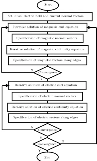
The suggested algorithm for attaining a numerical solution to Maxwell's equations is shown in Figure 1 and summarized as follows:
1. By using the initial amount of electric eld and current density on the nodes, their normal vectors on the surfaces of the grid are determined by averaging.
2. By using these normal amounts of electric eld and current density, the right-hand side of Eq. (24) is calculated for all grid surfaces. Then, this equation should be numerically solved for all surfaces. For attaining the numerical solution to this equation, an iterative method is applied. It means that for every surface, the elds on the left-hand side of Eq. (24) change in a way that this equation is satised for those surfaces. It means that the edges eld should change by Eq. (25).
Hi;l;new= Hi;l+
(RHS of Eq. (24)) P3
i=1
Hi;lLi 3
P
i=1Li
: (25)
The index \new" indicates the new amount of mag-netic eld obtained through iteration. Iterations continue until convergence is reached.
Figure 1. Suggested algorithm for attaining numerical solution to sinusoidal steady-state Maxwell's equations. 3. By new amount of magnetic eld along the edges,
new amounts of magnetic eld on the nodes and, then, normal to the surfaces are specied.
4. In order to increase accuracy of the result, the con-tinuity equation for magnetic eld in Eq. (22) must be satised. Similar to the method determined in stage 2, continuity equation must be satised iteratively.
In this case, new amounts of normal vectors should be changed in a way that continuity equation for the volume is satised. Thus, the following relation should be used:
Hi;n;new= Hi;n 4
P
i=1
Hi;nAi 4
P
i=1Ai
: (26)
Again, iterations continue until convergence is reached.
5. By new amounts of magnetic eld normal to the surfaces, new amounts of magnetic eld on the nodes and, then, along the edges are specied.
6. Stages 2 to 5 should be repeated until the results converge and satisfy both Eqs. (22) and (24).
7. Having normal vector of magnetic eld obtained through previous stages, the right-hand side of Eq. (23) is calculated. Then, this equation should be solved similar to Eq. (24) by the method that was mentioned in stage 2.
8. Normal vectors of the electric eld on the surfaces are specied as in stage 3.
9. Again, to increase the accuracy, the continuity equation for electric eld in Eq. (21) should be satised. This is done as in the method determined in stage 4.
10. Similar to stage 5, by new amounts of electric eld normal to the surfaces, new amounts of electric eld on the nodes and, then, along the edges are determined.
11. Stages 7 to 10 should be repeated until the results converge and satisfy both Eqs. (21) and (23).
12. Having new amounts of electric eld in the envi-ronment, stages 2 to 11 should be repeated until the results become convergent and satisfy Eqs. (21) to (24), simultaneously.
4. Validation of the method
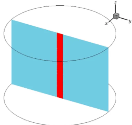
In order to validate the suggested method, a problem whose analytical solution is available will be numer-ically solved and the results will be compared with the analytical solution. A schematic of the problem is provided in Figure 2. A non-metal straight wire with radius of 0:1 (dimensionless units), located in the center of a cylinder with radius of 1:5 and height of 2, conducts a sinusoidal current with maximum amount of 1. The
Figure 2. The considered problem for validation of the method.
materials of the wire and the surrounding environment are considered to be dierent so that !L
c for wire is 1
and for surrounding environment is 0:1. The wall of the chamber is metallic, so normal magnetic eld and parallel electric eld on the wall are zero.
The analytical solution to this problem is (the details are discussed in the appendix):
8 > > > < > > > :
Ez= 1 1:0166J0(r) r 0:1
Ez=0:0041J0(0:316r)
+ 0:0080Y0(0:316r) r > 0:1
(27)
8 > > > < > > > :
H= 1:0166J1(r) r 0:1
H= 0:0013J1(0:316r)
0:0025Y1(0:316r) r > 0:1
(28)
where J0, J1, Y0, and Y1 are Bessel functions. This
problem is also numerically solved by the suggested numerical method. Figure 3 shows the grid used for the numerical solution. This grid consists of about 48000 nodes that are distributed with higher density around the surface of the wire where an acute change in the solution is expected. The same simulation is performed on two more resolved grids with the numbers of nodes of about 179000 and 312000 without any signicant change in the results, which means the solution is accurate enough with respect to the grid resolution.
Although the problem has axial and rotational symmetries, the numerical method does not exploit these symmetries. In other words, since the grid is unstructured, the numerical domain is not symmetric, and the symmetries and simplicity of the problem do not aect the numerical procedure. Therefore, a simple cylindrical geometry is used for validation of the method because of two reasons: rst, the simplicity of the problem is not relevant to the numerical method and, second, there is an analytical solution to this problem that can be referred to for validation.
Figure 3. The grid used for numerical solution to the case problem.
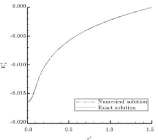
Figure 4. Comparison of the analytical and numerical solutions. The analytical and numerical solutions are very close to each other and it is dicult to distinguish them.
Figure 5. Comparison of the analytical and numerical solutions. The analytical and numerical solutions are very close to each other and it is dicult to distinguish them.
In Figures 4 and 5, the analytical and numerical solutions are compared. Based on these gures, the numerical solution is very close to the analytical so-lution. Since the grid is unstructured, simplicity of the problem does not aect the numerical solution. Therefore, it is concluded that the numerical approach is accurate enough, and can be used to solve Maxwell's equations.
5. Conclusion
A heuristic approach to numerically solve Maxwell's equations was suggested. This method was based on Yee's method, but could be applied to unstructured grids. This paper proposed the method for attaining a numerical solution to sinusoidal steady-state
prob-lems, but it is also possible to apply this method to fully unsteady problems. For unsteady problems, the suggested algorithm should be utilized in every time step. Further investigation could be done to increase the accuracy of the method by improvement of the transferring and averaging mechanisms.
Nomenclature
E -component of E
En Mean normal component of E on a
given surface
Er r-component of E
Ez z-component of E
Ei;l Mean parallel component of E on the
ith edge of a given surface
Ei;n Mean normal component of E on the
ith surface of a given volume
H -component of H
Hn Mean normal component of H on a
given surface
Hr r-component of H
Hz z-component of H
Hi;l Mean parallel component of E on the
ith edge of a given surface
Hi;n Mean normal component of H on the
ith surface of a given volume
Jn Mean normal component of J on a
given surface
Permittivity (C2.N 1.m 2)
^
J Order of imposed electric current density into the chamber
Permeability (N.A 2)
! Fields variation frequency (rad.s 1)
Electric charge volume density (C.m 3)
~E Dimensionless amplitude of electric eld vector
Y1 First order Bessel function of the
second kind
~H Dimensionless amplitude of magnetic eld intensity vector
~J Dimensionless amplitude of electric current density vector
~r Dimensionless location vector ~~E Amplitude of electric eld vector
~~H Amplitude of magnetic eld intensity vector (A.m 1)
~~J Amplitude of electric current density vector (A.m 2)
~
E Electric eld vector (V.m 1)
~
H Magnetic eld intensity vector (A.m 1)
~
J Electric current density vector (A.m 2)
~r Location vector (m)
Ai Non-dimensional area of the ith surface
of a given volume c Light velocity (m.s 1)
J0 Zero order Bessel function of the rst
kind
J1 First order Bessel function of the rst
kind
L Length scale of the chamber
Li Non-dimensional length of the ith edge
of a given surface t Time (s)
Y0 Zero order Bessel function of the
second kind
Acknowledgement
The authors would like to thank Dr. Asghar Molayi Dehkordi and Dr. Mehrdad Taghizadeh Manzari for their comments on the method suggested in this paper.
References
1. Yee, K. \Numerical solution of initial boundary value problems involving Maxwell's equations in isotropic media", IEEE Transactions on Antennas and Prop-agation, 14(3), pp. 302-307 (1966).
2. Taove, A. \Application of the nite-dierence time-domain method to sinusoidal steady-state electromagnetic-penetration problems", IEEE Transactions on Electromagnetic Compatibility, 3, pp. 191-202 (1980).
3. Taove, A. and Umashankar, K. \Radar cross section of general three-dimensional scatterers", IEEE Trans-actions on Electromagnetic Compatibility, 4, pp. 433-440 (1983).
4. Inan, U.S. and Marshall, R.A., Numerical Electro-magnetics: The FDTD Method, Cambridge University Press (2011).
5. Shang, J.S. \Characteristic-based algorithms for solv-ing the Maxwell equations in the time domain", IEEE Antennas and Propagation Magazine, 37(3), pp. 15-25 (1995).
6. Jahandari, H. and Farquharson, C.G. \A nite-volume solution to the geophysical electromagnetic forward problem using unstructured grids", Geophysics, 79(6), pp. E287-E302 (2014).
7. Lebedev, A.S., Fedoruk, M.P., and Shtyrina, O.G.V. \Finite-volume algorithm for solving the time-dependent Maxwell equations on unstructured meshes", Computational Mathematics and Mathemat-ical Physics, 46(7), pp. 1219-1233 (2006).
8. Fahs, H., Fezoui, L., Lanteri, S., and Rapetti, F. \Preliminary investigation of a nonconforming discon-tinuous Galerkin method for solving the time-domain Maxwell equations", IEEE Transactions on Magnetics, 44(6), pp. 1254-1257 (2008).
9. Um, E.S., Harris, J.M., and Alumbaugh, D.L. \3D time-domain simulation of electromagnetic diusion phenomena: A nite-element electric-eld approach", Geophysics, 75(4), pp. F115-F126 (2010).
10. Bossavit, A. and Kettunen, L. \Yee-like schemes on staggered cellular grids: A synthesis between FIT and FEM approaches", IEEE Transactions on Magnetics, 36(4), pp. 861-867 (2000).
11. Bossavit, A. and Kettunen, L. \Yee-like schemes on a tetrahedral mesh, with diagonal lumping", Inter-national Journal of Numerical Modelling Electronic Networks Devices and Fields, 12, pp. 129-142 (1999). 12. Sazonov, I., Hassan, O., Morgan, K. and Weatherill,
N.P. \Yee's scheme for the integration of Maxwell's equation on unstructured meshes", In ECCOMAS CFD 2006: Proceedings of the European Conference on Computational Fluid Dynamics, Egmond aan Zee, The Netherlands, September 5-8, 2006, Delft University of Technology; European Community on Computational Methods in Applied Sciences (ECCOMAS) (2006). 13. Lehner, G., Electromagnetic Field Theory for
Engi-neers and Physicists, Springer Science & Business Media (2010).
Appendix
Analytical solution to the considered problem First, the problem of a wire with innite length located in the center of a cylinder is considered. Because of the symmetry in the problem, the -direction and z-direction derivatives are zero, and the elds only depend on r-direction. As a result, Eqs. (15) and (16) yield:
0 = Hr; (A.1)
@ Ez
@r = Hheta; (A.2) 1
r @
@r(r E) = Hz; (A.3)
0 =
!L c
2
@ Hz
@r =
!L c
2
E; (A.5)
%1r@r@ (r H) =
!L
c 2
Ez+ Jz; (A.6)
Based on Eqs. (A.1) and (A.4), the r-components of the elds are zero. Boundary conditions for the problem are:
8 > < > :
E1;= bounded r = 0
E1;= E2;; H1;z= H2;z r = 0:1
E2;= 0 r = 1:5
(A.7)
8 > < > :
E1;z = bounded r = 0
E1;z = E2;z; H1;= H2; r = 0:1
E2;z = 0 r = 1:5
(A.8)
In these equations, the index 1 indicates the location inside the wire and the index 2 indicates outside of the wire. Based on Eqs. (A.3), (A.5), and the boundary condition (Eq. (A.7)), the -component of the electric eld and the z-component of magnetic eld are zero. Combining Eqs. (A.2) and (A.6) gives the nal equation for z-component of electric eld:
r2@2Ez
@r2 + r
@ Ez
@r +
!L c
2
r2E
z= r2Jz: (A.9)
This equation is the Bessel dierential equation whose analytical solution is available. Solving this equation for wire and the surrounding environment, separately, and using Eq. (A.2) give the analytical solution to the
innite-length wire problem: 8
> > > < > > > :
Ez= 1 1:0166J0(r) r 0:1
Ez=0:0041J0(0:316r)
+ 0:0080Y0(0:316r) r > 0:1
(A.10)
8 > > > < > > > :
H= 1:0166J1(r) r 0:1
H= 0:0013J1(0:316r)
0:0025Y1(0:316r) r > 0:1
(A.11)
Since in this problem, E, Er, and Hz are zero,
the solution satises the boundary conditions of the considered problem. Thus, the results satisfy Eqs. (15) and (16) and the boundary conditions of the considered problem. Consequently, the results of the case problem are the results of the innite-length wire problem. Biographies
Sajjad Azimi obtained his BS degree in 2012 and MS degree in 2015 in Mechanical Engineering from Sharif University of Technology, Tehran, Iran. He is now a PhD student at Ecole Polytechnique Federale de Lausanne, Lausanne, Switzerland. His elds of study are biouids, microfabrication, and boundary layer ows.
Mohammad Said Saidi received his PhD degree from Massachusetts Institute of Technology, USA, in 1979, and is currently Professor of Mechanical Engi-neering at Sharif University of Technology, Tehran, Iran. His research interests include, but are not limited to, CFD, micro and macro multiphase ows in human body, experimental design, and mathematical modeling of transport of nano- and micro-scale aerosol particles.