ABSTRACT
UNCMOBILE4 is a mobile source emission factor model that has been designed
to include the benefits of a fuel switch toward methanol fuel in future scenarios. UNCM0BILE4 is a modified version of EPA's emission factor modelM0BILE4. MOBILE4's overall structure is kept. Two vehicle classes, Light
Duty Flexible fueled vehicles running on Methanol (LDFM) and Light Duty
Flexible fueled vehicles running on Gasoline (LDFG), have been added to the
original eight vehicle classes of the EPA model. UNCMOBILE4 provides HC,
CO and NOx average emission rates from in-use methanol-fueled cars and from
vehicle fleets of changing composition under a wide range of conditions. The
LDFM and LDFG calculations are mostly based on data from Gabele (1990).
Some correction factor calculations are the same as for Light Duty Gasoline
Vehicles (LDGV) until explicit research data becomes available. The model has
been prepared in a way that the extensive but not yet released data from the
TABLE OF CONTENTS
1. Introduction 1
2. Methanol cars 3
2.1 Methanol car technology and economy 3 2.2 Composition of methanol car emissions 4
2.3 Methanol car emissions and urban ozone 5
2.4 Other environmental impacts 7
3. The current M0BILE4 Program 9 3.1 DataBase 10 3.2 M0BILE4 and UAM 10 3.3CLEAN4 11 3.4 Performance of M0BILE4 12 4.UNCMOBILE4 15 4.1 Technical differences to M0B1LE4 15 4.1.1 DataBase 16 4.1.2 Execution Summary 18
4.1.3 Modeling of emissions 22
Hydrocarbon exhaust
Hydrocarbon evaporative Hydrocarbon refueling losses
Hydrocarbon running losses
Carbon monoxide exhaust
Nitrogen oxide exhaust
4.2 User's guidance for UNCM0BILE4 31
4.3 Performance of UNCM0BILE4 335. Recommendations for further changes of UNCM0BILE4 36
6. Bibliography 38
Appendix A: UNCM0BILE4 Example Input 39
Appendix B: UNCM0BILE4 Example Output 40
Appendix C: Source code of subroutine EFCALX 41
Appendix D: Source code of subroutine HCCALX 45
Appendix E: Source code of subroutine EVMET 50
LIST OF ABBREVIATIONS
ATP Anti-Tampering Program
CF Correction Factor CO Carbon Monoxide
DR Deterioration Rates
EPA (U.S.) Environmental Protection Agency
EF Emission Factor
FFV Flexible Fueled Vehicles (=LDF)
FTP Federal Test Procedure
gpg grams per gallon gpm grams per mile HC (total) Hydrocarbons
HDDV Heavy Duty Diesel Vehicles HDGV Heavy Duty Gasoline Vehicles LDDT Light Duty Diesel Trucks LDDV Light Duty Diesel Vehicles
LDF Light Duty Flexible Fueled Vehicles
LDFG Light Duty Flexible Fueled Vehicles running on gasoline
LDFM Light Duty Flexible Fueled Vehicles running on M85
LDF Light Duty Flexible Fueled Vehicles (=FFV) LDGTl Light Duty Gasoline Trucks class 1
LDGT2 Light Duty Gasoline Trucks class 2 LDGT Light Duty Gasoline Trucks
LDGV Light Duty Gasoline Vehicles
M85 Blend of 85% methanol and 15% gasoline
MC Motorcycles
mpg miles per gallon
NOx Nitrogen Oxides, sum of nitrogen monoxide and niti^ogen dioxide RVP Reid Vapor Pressure
SIP State Implementation Plan VRS Vapor Recovery System
1. INTRODUCTION
Mobile source's emissions of hydrocarbons, nitrogen oxides, and carbon monoxide are considered to be important contributors to urban ozone. Control
devices for gasoline cars have been employed to reduce emissions of new and in-use vehicles by 92 and 78 percent, respectively, over the past 20 years. The associated
development of new vehicle emission standards is shown in TABLEl. Further
efforts to reduce emissions from cars powered with conventional gasoline "must now
contend with a law of diminishing returns" [Gabele, 1990].
Cleaner fuels are currently being examined to determine their ability to
improve air quality. Alternative, carbon-based fuels might have the potential to mitigate urban ozone and carbon monoxide levels during the inevitable transition
toward electrically-powered and hydrogen-powered transportation. At this time, the most promising alternative fuel with both economically and environmentally attractive attributes appears to be methanol [Gabele, 1990]. Methanol fuels are also
being considered because of their ability to reduce American dependency on foreign oil and to reduce gases contributing to global warming.
As a crucial step in determining future air quality, complex photochemical
models such as the Urban Airshed Model need realistic and reliable emission
inventories for in-use highway fleets. For this task, the United States Environmental Agency developed the MOBILE series of vehicle emission rate models of which M0BILE4 is the latest version. M0BILE4 is a very complex set of 151 FORTRAN
subroutines, functions, and block data which calculates emission factors in units of
g/mile under a wide range of user-specified environmental conditions.
This paper introduces the vehicle emission model UNCM0BILE4 that has been designed to be able to include the benefits of a fuel switch toward methanol
blends in future scenarios. UNCMOBILE4 is a modified version of EPA's
MOBILE4 and provides additionally HC, CO and NOx emission rates from in-use methanol-fueled cars and from vehicle fleets of changing composition under a wide range of conditions.
Two vehicle classes, Light Duty Flexible fueled vehicles running on Methanol
(LDFM) and Light Duty Flexible fueled vehicles running on Gasoline (LDFG),
have been added to the original eight vehicle classes of the EPA model. While the
overall structure of MOBILE4 is kept, numerous subroutines had to be changed and
many others added to account for base emission rates and dependencies different
Introduction_________________________________________________________________________UNCMODII,i:4
TABLE 1: Exhaust and evaporative emission standards for new Light Duty
Vehicles
Exhaust Exhaust Exhaust Evaporative
Year HC CO NO^ HC
1972 3.4 gpm 39 gpm
-2.0 g/test
1973-74 3.4 gpm 39 gpm 3.0 gpm 2.0 g/test
1975-76 1.5 gpm 15 gpm 3.1 gpm 2.0 g/test
1977 1.5 gpm 15 gpm 2.0 gpm 2.0 g/test
1978-79 1.5 gpm 15 gpm 2.0 gpm 6.0 g/test
1980 0.41 gpm 7 gpm 2.0 gpm 6.0 g/test
1981 3.4 gpm 3.4 gpm 1.0 gpm 2.0 g/test
Notes:
1 Different test procedures have been used since the early days of emission contol which vary in stringency. The appearence that standards were relaxed is incorrect and arises from test
procedure changes.
UNCMOBILE4 cannot yet be assumed to provide reliable emission factors for future methanol cars since it is not based on the most recent data and it partly
reUes on unchecked assumptions. So far, mostly data from Gabele (1990) has been utilized. Thus, the model has been prepared in a way that the extensive but not yet released data from the Auto/Oil study on flexible fueled cars can be inserted. UNCMOBILE4 can also serve as a pattern for including other vehicle classes
2. METHANOL CARS
2.1 Methanol Car Technology and Economy
Flexible fueled vehicles (FFV) are designed for using gasoline fuel or any alcohol/gasoline blend up to 85% methanol. An electronic sensor in the fuel
delivery system senses the methanol content of the mixture, and engine parameters
are adjusted appropriately for proper combustion. Like all methanol cars, they also
need modified fuel tanks and fuel delivery systems to withstand methanol's corrosive
nature. Although FFV cannot provide the same emission benefits as dedicated
vehicles, they are likely to be used during a transition period when gasoline is
phased out and alternative fuel is phased in.
Dedicated methanol vehicles can only use fuel composed of at least 85%
methanol. These vehicles, if running on MlOO (100% methanol), promise the greatest emission benefits but are difficult to start at ambient temperatures below 60 F. If this problem can be solved, they might become the best option for future use.
Because of its high oxygen content methanol contains only about one-half of
the energy per gallon of gasoline. Thus, methanol cars yield comparably much lower
miles per gallon values. But other properties make methanol a more energy efficient fuel than gasoline. Its higher octane rating permits a higher compression ratio, its wide flammability limits allow good combustion while operating lean, and its higher energy output permits smaller engines while providing the same performance. These effects are believed to add up to a 30 percent increase in overall vehicle efficiency for dedicated vehicles. [EPA, 1989]
Methanol fuel prices can be competitive with gasoline at current world oil
prices. M85 pump prices could be 68 to 74 cents per gallon, including costs for distribution, retail markup, and fuel taxes. The lower energy content of M85 and its
slightly higher efficiency yield to a projected gasoline retail price equivalent of 114
to 124 cents per gallon. MlOO's pump price could be 60 to 67 cents per gallon.
Considering the lower energy content and the 30 percent higher efficiency expected
for an optimized, dedicated vehicle, the projected gasoline retail price equivalent
yields to 92 to 103 cents per gallon. The retail prices can be lowered even further if
methanol is produced on larger scale. Thus, the price for M85 and MlOO is
competitive with todays gasoline prices and even lower than those for premium
gasoline, which is the natural competitor for the high octane methanol fuels
Introduction__________________________________________________________________________________UNCMOBILE4
EPA estimates the costs for dedicated methanol vehicles as the same as for
future gasoline vehicles. Flexible fueled vehicles might be up to $300 more
expensive, among other things because a fuel sensor is needed [EPA, 1989].
2.2 Composition of Metlianol Car Emissions
The precise forecasting of emissions from future methanol cars and fleets is
extremely difficult, since the emissions depend on numerous factors. Exhaust,
evaporative, refueling, and miming loss emissions are substantially different for
dedicated methanol vehicles and flexible fueled cars. For the latter ones, the
emissions are a factor of the fleet portion actually rurming on a methanol blend, and for both vehicle classes a function of the gasoline content of the fuel supplied.
The methanol car technology is still evolving, and parameters for the
eventual, optimized methanol vehicle are not yet known. The emission levels finally attainable and the cars fuel efficiencies are still hard to predict. Also emission standards and required control technologies as well as which vehicle classes will be
affected is not yet exactly known.
There is strong evidence that far lower emissions than for gasoline vehicles
finally can be achieved by at least certain kinds of methanol vehicles [EPA,1988]. Therefore future standards for these cars might adjust to the advanced technology. The currently proposed standards for light duty methanol vehicles are the same as for LDGV, for HC on a carbon mass basis [Dunker, 1990]. Modeling on the basis of
these standards would mean that only the composition of the emitted hydrocarbons
changed. The other approach, taken by UNCMOBILE4, is to utilize actual test data
for calculating the model's base emission rates and corrections.
Whether or not methanol vehicles will play a role as a future vehicle fuel,
and the applied technology, and the future emission rates, are a function of
enviroimiental and economic policies on federal and state level. A switch to any kind of alternative fuel requires major and cost-intensive changes and perhaps market share losses in two of the biggest and most influential industrial branches.
The automobile industry and possibly even more the oil industry will be highly
affected. They might prefer a transition to oxygenated fuels, so strong opposition
might arise from them.Nevertheless, a number of research projects on methanol cars have been
conducted and allow qualitative and quantitative assessment of their emissions. It
Introduction__________________________________________________________________________________UNCMOBILE4
ozone forming potential, is the composition of the emissions and to a lesser extend
their absolute amounts.
The emissions from flexible fueled vehicles running on MO, that is pure gasoline, are generally considered to be the same as for regular light duty gasoline vehicles. Blends containing more methanol produce similar amounts of exhaust regulated emissions (organic material, carbon monoxide, and nitrogen oxides). Ambient temperature affects the emission rates in the same matter as for gasoline cars: organic and CO emissions increase strongly at lower temperatures whereas NOx is less affected. Mass exhaust emissions stay virtually constant above 75 F.
[Gabele, 1990]
Gabele (1990) tested flexible fueled cars with MO, M25, M50, M85, and MIOO. He states that, while increasing the fuel's methanol content, "formaldehyde and methanol comprise increasingly greater portions of the material while hydrocarbons comprise less." Both compounds also increase strongly at lower temperatures. [Gabele, 1990] Testing an early model FFV, Gabele found that benzene, 1,3-butadiene, and acetaldehyde emissions are lower for M85 use than for MO use. Exhaust methane increases with increasing methanol content, whereas the composition of the remaining hydrocarbons is not significantly affected. Gabele found similar portions of paraffins, olefins, and aromatics of total HC for MO and
M85. [Gabele, 1991]
Evaporative emissions increase with fuel volatility, that is with decreasing
methanol content, and increase with temperature. Diurnal emissions are much greater in magnitude and more sensitive with respect to temperature and fuel volatility than hot soak emissions. The gasoline portion of methanol fuel blends, even if small, contributes significantly to the emissions. 40 % of the M85 exhaust carbon is gasoline related. [Jeffries, 1991] Gabele also found the hydrocarbon
component of evaporative emissions from M85 to dominate over the methanol
component. [Gabele, 1990]
Methanol is released into the atmosphere as unburned fuel in exhaust and
evaporative emissions. Aldehyde derivates such as formaldehyde are combustion products in the exhaust gas. A great portion of the total formaldehyde emissions occur during the first part of the cold start mode. [Gabele, 1990]
2.3 Methanol Car Emissions and Urban Ozone
Introduction_________________________________________________________________________UNCMOBILE4
Quality Standard (NAAQS) for ozone is a 1-hour averaged concentration of ozone of 0.12 ppm not to be exceeded more than once per year at any location over a three year period. It is still violated in 60 major urban areas in the United States. Los Angeles has exceeded the standard in the late eighties some 140 times per year
(Seinfeld, 1988).
The hope that a switch toward methanol as an automobile fuel could reduce
ambient ozone levels arises mostly from the altered composition of the alternative fuel exhaust and particularly of its organic emissions. The volatile organic compounds (VOC) are expected to show a lower degree of reactivity than those from gasoline emissions. Methanol makes up a large portion of the organic exhaust and evaporative emissions and is considered to have a much lower reactivity than other organic compounds. The fraction of methane, another low reactive compound, is increased for methanol vehicles. Also formaldehyde is emitted at a higher rate than by gasoline cars. Formaldehyde is considered to be a very reactive compound
and a strong source of radicals.
Extensive research projects are underway to verify and quantify the benefits of the relative reactivity of methanol car emissions. They utiHze smog chamber experiments and complex photochemical models such as the Urban Airshed Model (UAM). It is difficult to reliably predict the effects of alternative fuels because of
the complexity of the concept of reactivity.
Reactivity is defined as "the extent to which a compound or a mixture of
compounds contributes to atmospheric oxidation of VOC, oxidation of NO to NO 2, and subsequent O3 production in the ambient atmosphere" [Jeffries et al., 1991]. It arises from complex interactions among all reacting species. Thus, it is a non-linear function of numerous atmospheric conditions such as the NOx-HC-ratio, and any
"reactivity scale" for VOC compounds is necessarily relative.
To illustrate the complexity of the issue, Jeffries states that most of the ozone
is formed by the least reactive compounds. CO, methane, and alkanes, form up to
half of the urban O3 simply because of their high concentrations. Highly-reactive
species such as olefines, xylenes, and emitted aldehydes are the primary source of
"new radicals", which are required for ozone formation. The reactions for only very few of these compounds are precisely understood. Thus, further research has to be done to refine the chemical mechanisms utilized in the computer models that could evaluate alternative fuels. [Jeffries et al., 1991]
Currently, alternative fuels can be included in future air quality scenarios and
Introduction_________________________________________________________________________UNCMOBILE4
Motor Vehicle Emission Reductions from the Use of Alternative Fuels and Fuel
Blends" (1988), and represent relatively old research data. This document describes methods and assumptions for estimating the impact from the use of gasohol. Methyl Tertiary Butyl Ether (MTBE) blends, compressed Natural Gas (CNG), and
methanol blends - including M85 and MlOO - on vehicle HC, CO, and NOx
emissions.
The actual credit for methanol car use would depend on the emission levels
of the proposed vehicle technology for that area. EPA specifies the reductions for methanol vehicles just meeting the emission standards, for those well below the
standards, and for those with intermediate emission levels. The credit is to be applied to MOBILE4's non-methane HC exhaust and evaporative model year
emission factors; CO and NO^ emission levels are unchanged.
2.4 Other Environmental Impacts
Whereas all carbon-based fuels necessarily emit gases contributing to the greenhouse effect, their amount can be reduced if gasoline is replaced by alternative
fuels. Whether using methanol could yield global warming benefits, depends mostly on the way it is produced.
Currently, the production from natural gas is economically favored. If natural
gas which is now vented or flared is used, a large warming benefit will accrue, since
such gas is currently being wasted while adding huge amounts of carbon dioxide and
methanol to the greenhouse gas burden. Using coal as a methanol feedstock with current technologies could nearly double greenhouse gas emissions due to large losses at the mine and at the production plant. The greatest benefit would arise from using cellulose, biomass or other renewable feedstock, since such materials are not stored carbon. Their growth would remove the same amount of carbon dioxide
from the atmosphere as their combustion would emit. [EPA, 1989]
Significant reductions in the number of cancer cases are projected for
replacing gasoline by methanol since emissions of hydrocarbon air toxics such as benzene, 1,3-butadiene or polycyclic aromatic matter would be reduced or
eliminated. Methanol is not generally considered a toxic air pollutant.
Formaldehyde is classified by EPA as a probable human carcinogen. This issue is
often raised as a concern since the levels of initially emitted formaldehyde are
higher for tested methanol cars, even though control technology could reduce them
to gasoline levels. Methanol is not expected to increase the number of cancer cases
Introduction__________________________________________________________________________________UNCMOBILE4
3. THE CURRENT MOBILE4 PROGRAM
MOBILE4 is a computer program designed to estimate average mobile
source emissions in units of g/mile. The model provides both current and future
emission rates from highway vehicle fleets under many environmental conditions. The model weights emissions from vehicles of the most recent 20 model years to obtain fleet emissions as of January 1 of the requested calendar year. The emission
factors are adjusted to compensate for numerous factors. Speed, temperature, and
cold/hot driving mode mix are most influential, tampering and fuel volatility also
have a major impact.The results are split into the following compound classes: total HC, exhaust HC, evaporative HC, refuel losses HC, running losses HC, exhaust CO, and exhaust NOx- The emission factors are also specified for eight vehicle classes: Light Duty Gasoline Vehicles (LDGV), Light Duty Gasoline Trucks 1 (LDGTl), Light Duty Gasoline Trucks 2 (LDGT2), Heavy Duty Gasoline Vehicles (HDGV), Light Duty Diesel Vehicles (LDDV), Light Duty Diesel Trucks (LDDT), Heavy Duty Diesel
Vehicles (HDDV), and Motorcycles (MC).
MOBILE4 consists of an integrated set of 151 FORTRAN subroutines. It is
the most recent of EPA's MOBILE series of motor vehicle emission factor models.
MOBILE4.1, which allows the evaluation of oxygenated fuels, is expected to be
released very soon.
MOBILE4 provides a flexible analytical tool for a wide range of air quality planning functions. Except for California, EPA requires the motor vehicle emission inventories in all ozone, CO, and NO 2 SIP revisions to be based on the latest MOBILE version.
MOBILE4 suppUes four types of formatted reports. Two types of "numeric"
output are suitable for use as an input file for subsequent computer analysis. Two
types of "descriptive" output are more suitable for visual inspection and analysis and
MOBILE4___________________________________________________________________^___________UNCMOBILE4
3.1 Database
The program uses the calculation procedures and extensive emission factor data presented in EPA's "Supplement A to Compilation of Air Pollutant Emission
Factors - Volume II: Mobile Sources" (1991). For current exhaust emission rates, dynamometer tests under conditions of the Federal Test Procedure (FTP) were performed. The data is specified into three sampling bags for the three operating
modes: cold start, hot start, and hot stabilized mode. New as well as on-road
vehicles were tested to determine zero mile level and deterioration rates.
Exhaust, hot soak, diurnal, crankcase, refueling loss, and running loss emissions as well as idle exhaust emissions were determined. Special emission testing programs were performed to determine various correction factors. For future
emission rates, federal new-vehicle emission standards based on FTP are assumed.
M0BILE4 contains extensive driving pattern data from chase car surveys determining the mix of operating modes as a function of average route speed as well
as data for trips per day and miles per trip.
3.2 Mobile4 and UAM
MOBILE4 is utilized to provide mobile sources emission input for complex
photochemical air quality models such as SAI's Urban Airshed Model (UAM), and thus is a crucial step in predicting future air quality, and in evaluating control
strategies.
For use in the UAM, mobile sources inventories must be temporally,
spatially, and chemically resolved to the level of the other modeling inputs: cells of 4 to 25 km2 for hourly emission estimates in species recognized by the Carbon Bond
Mechanism Version IV (CB4).
This is done by the UAM's Emission Preprocessor System (EPS) which
produces a gridded binary emissions file for input in the UAM. The emissions are allocated to the grid cells of the modeling region and split into the CB4 species NO,
NO2, OLE, PAR, TOL, XYL, FORM, ALD2, ETH, MEOH, ETOH, and ISOP.
The applied factors are derived from EPA's Air Emission Species Manual (1988).
The emission rates are transformed into hourly emission rates by diurnal variation
factors and adjusted for the weekday by weekday variation factors. Among other
data, HC, CO, and NO^ exhaust and evaporative emission factors, fractional vehicle
miles travelled (VTM) and motor vehicle adjustment factors generated by
MOBILE4 are is used as input for EPS.
MOBILE4________________________________________________________________^_______UNCMODILR4
3.3Clean4
Based on MOBILE4, EPA developed CLEAN4, an emission factor model for evaluating "clean fuels". It applies adjustments that account for emission reductions from any two kinds of alternative fuel, for instance from M85 and MlOO
fuels.
The emission reduction factors for HC, CO, and NOx, and for diurnal, hot soak, refueling, and running loss emissions are specified by the user in the one-time data entry. CLEAN4 does not contain any estimates of the effect of alternative
fuels, but supplies the algorithm for evaluating them. The user also specifies sales
fractions for the two alternative fuel vehicle classes for model year from 1993 on. The adjustments are applied as multiplicative correction factors to light duty
gasoline vehicle and trucks' emission factors. Thus, all internal MOBILE4
corrections apply unchecked as well for the "clean" vehicles. CLEAN4 does not
MOBII,H4 UNCM0BILn4
3.4 Performance of M0BILE4 '
The sensitivity of M0BILE4's output emission factors for several input parameter
is shown in FIGURE 1 through FIGURES.
2.4
2.2
~ 2.0 h U)
1,
Q 1.6
o cd o
'^ 1.2
Q) 1.0 B
M 0.8 o
a
E 0.6 o
o
0.4
0.2
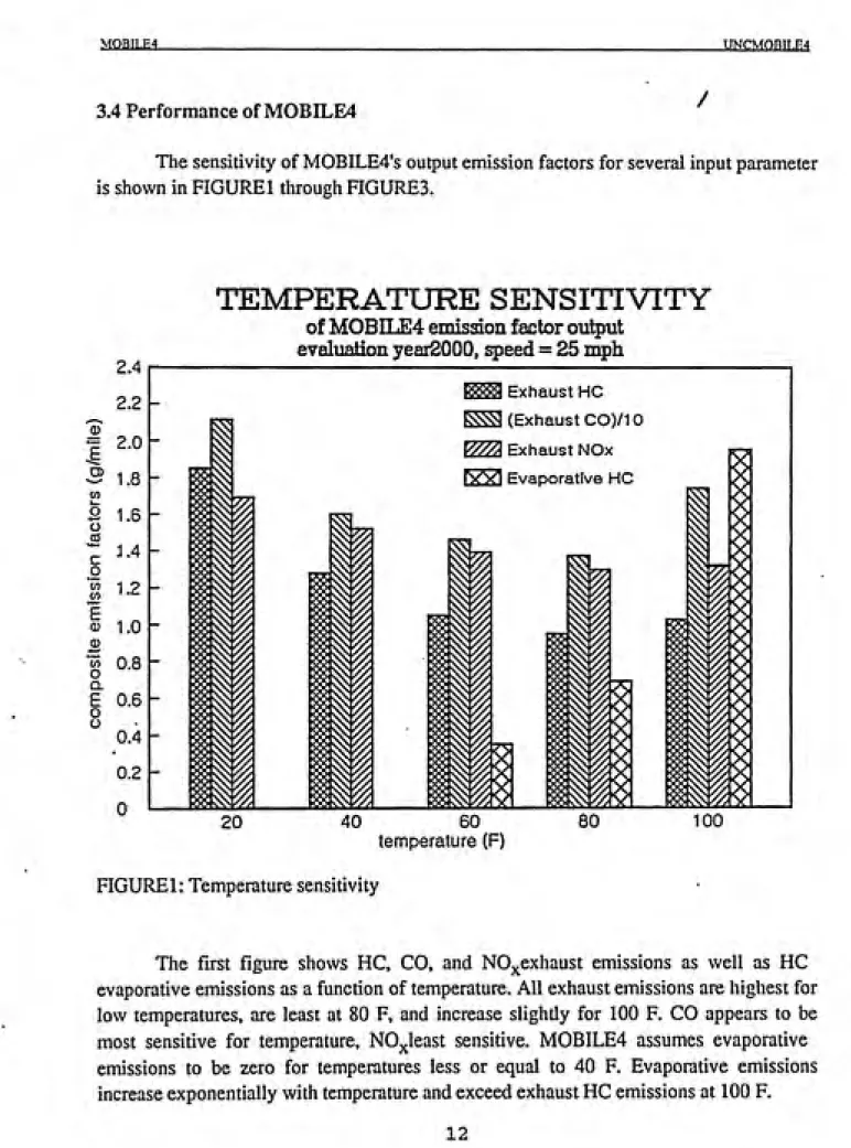
TEMPERATURE SENSITIVITY of M0BILE4 emission factor output
evaluation yeaiSOOO, speed = 25 mph
Exhaust HC
^S (Exhaust CO)/10
P?^ Exhaust NOx
rWI Evaporative HC
20 40 60
temperature (F)
80 100
FIGURE 1: Temperature sensitivity
The first figure shows HC, CO, and NOj^exhaust emissions as well as HC evaporative emissions as a function of temperature. All exhaust emissions are highest for low temperatures, are least at 80 F, and increase slightly for 100 F. CO appears to be
most sensitive for temperature, NOj^least sensitive. M0BILE4 assumes evaporative
MOBILE4 UNCMORTI.E4
E
3
i
_ 5
4
c
.2 3
"6
<p
ͣ
^ 2
o o.
E
8 .
SPEED SENSITIVITY
of M0BILE4 exhaust emission factor output evaluation year 2000, temperature = 80 F
FIGURE2: Speed sensitivity
Exhaust HC
1^^ (Exhaust CO)/10
P^^^ Exhaust NOx
25 35 speed (mph)
Exhaust emissions are also a function of average vehicle speed. M0BILE4
MOBILE4 UNCMOB11-H4
EVALUATION YEAR SENSITIVITY
of M0BILE4 exhaust emission factor output
temperature = 80 F, speed = 25 mph
^ 4 05
3
-u.
O
.-•
o
i5
c g
'w
w
"E
<D CD W O Q.
E o 1
Exhaust HC
g^^ (Exhaust CO)/10
K^^ Exhaust NOx
li
1982 1992 2002
evaluation year
2012
FIGURES: Evaluation year sensitivity
The emission factors decrease with time, as shown here for fleet average
composite exhaust HC, CO, and NOx emission factors. The per-cai- emissions decrease since older vehicles, built for higher emission standards, phase out and are replaced by
newer vehicles. MOBILE4 does not contain projections for lower future emission
standards. The zero mile emission levels for future cars are assumed to be the same as for
current vehicles since no explicit information on future standards is available yet. Therefore, the calculated emissions approach and finally reach a constant level, after all
old higher-standard vehicles are replaced.
However, it is important to note that MOBILE4 models average per-cai" emission factors rather than summed-up total emissions from the entire fleet. Total fleet emissions
might stay constant or even go up despite of decreasing average emission levels, if the
number of vehicles grows.
UNCMOBILE4_______________________________________________________________________________UNCMOBIT,E4
4.UNCMOBILE4
4.1 Technical Differences to M0BILE4
The vehicle emission model UNCM0BILE4 has been developed to include
flexible fueled cars in future vehicle fleet emission scenarios. It is a modified version of
EPA's M0BILE4 which does not offer this opportunity.
Two vehicle classes. Light Duty Flexible fueled vehicles running on Methanol
(LDFM) and Light Duty Flexible fueled vehicles running on GasoHne (LDFG), have
been added to the original eight vehicle classes of the EPA model. Thus, the calculation
of composite emission factors becomes possible for a vehicle fleet stepwise or partly switched toward methanol vehicles. The user only needs to specify annual sales fractions for FFV, the portion of FFV actually running on M85, M85's Reid Vapor Pressure, and to set two execution controlling flags.
The calculations for the eight old classes are kept unchanged. Only their vehicle
miles travelled (VMT) share is reduced by the internal calculated VMT portion of LDFM
and LDFG for each calendar year. As far as the currently available FFV emission factor
data allows, the LDFM and LDFG calculations follow the pattern of those for the LDGV. Since this data is not as detailed as those utiUzed by M0BILE4, they are simplified at
some points. Other correction factor calculations are taken unchanged from LDGV until explicit research data becomes available, if they can be assumed to be similar. Driving pattern data such as vehicle age specific accumulated mileage, trips per day, and miles
per day are the same as for LDGV. It is important to note that UNCM0BILE4's HC emission factor output reflects the total organic emissions, including hydrocai'bons, methanol, and formaldehyde.
The advantage of keeping the original MOBILE4 structure is that as soon as new
data such as those from Auto/Oil becomes available, it can easily be included in
UNCM0BILE4's data basis. Depending on the nature of this data, further changes to the
algorithm might be conducted. The LDF calculations finally become as sophisticated and detailed as for the other vehicle classes. This is unlike EPA's CLEAN model which only applies multiplicative correction factors to M0BILE4's vehicle classes to account for
emission reduction due to alternative fuels. UNCM0BILE4 can also serve as a pattern
for including other vehicle classes instead of, or additional to, FFV into M0BILE4 or
UNCMOB1LE4________________________________________________________________________________UNCM0BILE4
No information is available yet about in-use tampering rates and tampering effects for FFV. Nevertheless, it appears to be necessary to include tampering in the emission factor calculations since the arising excess emissions can be considerable. UNCM0BILE4 provides the opportunity to consider those effects for either one or both
of the vehicle classes. If the control flags are set appropriately, tampering is assumed to
add the same portion to the non-tampered emissions as for LDGV.
FFV running on gasoline are usually believed to produce the same g/mile emissions as LDGV. Depending on a control flag setting, all LDFG model year emissions can be set equal to those for conventional gasoline vehicles of that model year. Differences between LDGV and LDFG composite emission factors then arise only from
different age distributions, that is registration mixes for the two classes.
The optional user input opportunities provided by M0BILE4 are not yet fully
extended to cover the two new vehicle classes. The use of some of the control section
flags is restricted to keep the comparability of the new and the old classes.
4.1.1 Data Base
The basic emission rates and correction factors for LDFM and LDFG calculations are mostly based on data published by Gabele (1990) who examined emissions from FFV. He measured HC exhaust and evaporative emissions as well as CO and NOx exhaust emissions for the gasoline/methanol blends MO, M25, M50, M85, and MlOO at
40 F, 75 F, and 90 F.
The test vehicle investigated was a 1988 General Motors Variable Fuel Corsica
with a 2.8-1 six cylinder engine having a compression ratio of 8.9:1. The fuel system was
port injection, the control loop was closed, and the mileage was 4500 miles. The test
fuels were MO (100% gasoline, 0% methanol) and M85 (15% gasoline, 85% methanol).
The gasoline portion was indolene (certification fuel), the methanol was of laboratory
grade specification. MO had a Reid Vapor Pressure (RVP) of 9.0, M85's RVP was 8.0.
The fuel economy was 22.0 mpg running on MO and 13.4 mpg running on M85.
Data on emission rates and fuel economy were obtained both the Federal Test
Procedure (FTP) and the Highway Fuel Economy Test. Three replicate tests were run for
each temperature/fuel type combination. The organic emissions are calculated in
accordance to the carbon mass equivalent method. The HC data utilized in
UNCMOBILE4________________________________________________________________________________UNCMOBILE4
TABLEl: Exhaust emissions (g/mile)
HC CO NOx
40 F
FFV on M85 1.86 8.50 0.28
FFV on MO 0.93 8.80 0.20
75 F
FFV onM85 0.43 2.60 0.26
FFV on MO 0.32 2.60 0.22
90 F
FFV on M85 0.51 2.40 0.31
FFV on MO 0.36 2.8 0.26
TABLE2: Hot soak and diurnal emissions (g/test)
HS DU
40 F
FFVonM85 0.14 0.19 FFV on MO 0.19 0.26
75 F
FFVonM85 0.25 0.49 FFV on MO 0.28 0.54
90 F
UNCMOBILE4________________________________________________________________________________UNCMOniLI-:4
TABLE3: Non-methane portion of HC exhaust
40 F 75F 90F
FFVonM85 0.85 0.75 0.81
FFVonMO 0.90 0.90 0.87
The basic emission rates and correction factors for LDFM and LDFG calculations are mostly based on data published by Gabele (1990) who examined emissions from
FFV. He measured HC exhaust and evaporative emissions as well as CO and NOx exhaust emissions for the gasoline/methanol blends MO, M25, M50, M85, and MlOO at
40 F,75 F, and 90 F.
4.1.2 Execution Summary
UNCM0BILE4's structure and thus also the program execution are virtually the same as M0BILE4's. Its source code consists of 158 subprograms. These subroutines, functions, and block data are called by the program's driver MAIN or by other
subprograms and may in turn call other subprograms. MAIN loops through three
sections: input, calculation, and output. The most important subroutines are briefly
described below. Subroutine's names are written in upper case.
Input
This section reads in the input and prepares the parameters and data for the
subsequent calculation section. During one run, UNCM0BILE4 can evaluate several
different scenarios, but only the first scenario can include methanol cars. The program
utilizes one input data set that provides program control information and the data describing the scenarios. The user determines by the setting of the first flag (PROMPT)
whether the program reads in by prompting the user for each following input or by
reading a prepared, formatted input file. The input data set consists of three distinct
sections.
UNCMOniLM________________________________________________________________________^_________UNCMOBII.E4
input, output format, and execution of the program and consists of 17 flags. The flag setting also controls the format of the remainder of the input stream format of the output.
The One-time section is optional and is used to alter internal UNCM0BILE4
estimates to be locality-specific. This can include information on tampering rates, annual mileage accumulation rates or registration distributions by vehicle tjrpe and age, base emission rates, VMT mix, tampering parameters, inspection and maintenance program
credits, anti-tampering program parameters, refuelmg emission controls, fuel volatility,
and flexible fueled cars. ONESEC checks the flag values whether one-time data is
expected and reads it in by calling other subroutines. This data is used for all scenarios of
a run and replaces the corresponding default values hardcoded in BLOCK DATA.
GETMET reads in the methanol car related user input. It screens the values for being in
the ranges expected and calls QUITER if not.
The Scenario section details the individual scenarios of a run and reads in, among others, information on calendar year of evaluation, temperature, region (high or low altitude), and average speed by repeating PARS EC, GETSCl, and LOCAL for each scenario. LOCAL applies the same weathering to M85's RVP as to gasoline's RVP. Here calculated exhaust and evaporative temperatures are later also applied to LDF.
REGMOD calculates the evaluation year January 1 registration mix for the
vehicles of each model year. LDGV's and LDDV's share is reduced by LDF's sales share of that model year, the light duty gasoline/diesel ratio stays the same. REGMOD also figures the vehicle age specific mileage accrual rates and evaluation year January 1 accumulated mileages. From that, REGMOD constructs vehicle age and class specific miles per day and trips per day values. In UNCM0BILE4, the data underlying these
driving pattern calculations is the same for LDF and LDGV. YRTEST checks whether given years are in the allowed ranges. QUITER prints out error, warning, or comment
messages and, depending on the severity of an error, may terminate the run.
Calculation
This section generates the requested composite emission factors. The calculation
is performed for each vehicle type, each model year, and each of the compound classes. The algorithms for the two new vehicle classes are virtually the same as for LDGV and
are described in detail in Chapter 4.1.3.
Base exhaust emission rates are calculated from the zero mile levels and
UNCMOBII.F,4_______________________________________________________________________________ UNCM0BILE4
fractions to generate emission factors by vehicle type and pollutant class, and then again
weighted together by the normalized vehicle miles travelled (VMT) to produce a composite emission factors for each pollutant for the requested calendar year.
The calculation section is driven by EFCLAX. Fkst, additive offsets and
multiplicative correction factors are assembled in each scenario. GETCUM generates the
average January 1 cumulative mileage distribution. TAMPER, by contioUing the 16
tampering-related group of subroutines and functions, calculates tampering rates and
emission impacts. BIGCFX and the associated subroutines figure the correction factors
and corrections for speed, temperature, Reid Vapor Pressure (RVP) etc.
HC emission factors are calculated by HCCALX. It loops through each vehicle type and model year case, computing, correcting, weighting, and adding that case's
contribution to the composite results. IGSFPT provides the gas/diesel sales fraction,
IMSFPT points the LDF sales fraction year groups. BEF extracts the basic exhaust
emission rate and applies correction factors. LDF exhaust emission factors are corrected
for temperature by function EXTCOR. Function CH4COR determines the
temperature-specific non-methane portion.
CCEVRT returns evaporative HC emission factors for all gasoline and methanol vehicles and motorcycles utilizing HOTSOK (hot soak emissions), DIURNL (diurnal),
and CRANKC (crankcase), weighted by trips per day and miles per day. LDF hot soak
emissions are extracted by subroutine EVMET and EVRVPC, and temperature corrected
by function EVTCOR. RULOSS provides the running loss HC emission factors for gasoline and methanol vehicles. The refueling loss HC emission factors for the same vehicle classes are looked up in the table previously calculated by REFUEL. For
calculation of CO and NOx emission factors, EFCALX loops through each pollutant,
vehicle type, and model year case, utilizing BEF.
Output
On each successful scenario pass, OUTPUT routes the results to report unit 4.
0UTHD4 echoes the run title and the field headers. Subroutines echo the optional user
supplied input, like OUTMET does for methanol car input. OUTPOL selects which
pollutant's values are to be printed, and 0UTDT4 prints out user-supplied scenario data
and the calculated emission factors.
Subroutines GETMET, IMSFPT, EVMET, EVRVPC, EVTCOR, EXTCOR,
UNCMOBTLE4________________________________________________________________________________UNCMOBILE4
and extended. Most subroutines experienced minor changes. EFCALX, HCCALX,
UNCMOBILE4_______________________________________________________________________________UNCMOBII.F,4
4.1.3 Modeling of emissions
Hydrocarbon exhaust emissions
HC exhaust emissions are modeled for all vehicle classes. In MOBILE4 as well as
in UNCMOBILE4, they depend on vehicle mileage, temperature, tampering effects,
speed, location-specific adjustments, and the fuel's RVP.
The uncorrected base emission rate for each model year/vehicle class group is
determined from zero mile emission level (zml) and the deterioration rate (dr). Zml
(g/mile) and dr ((g/mile)/l 0,000 miles) are assumed to be the same for both low and high
altitude and are assumed to be constant for all model years.
The zero mile levels for LDFM and LDFG are the test results for the flexible
fueled test vehicle investigated under Federal Test Procedure (FTP) conditions by Gabele (1990), running on M85 and MO, respectively. Since there is no data on deterioration rates yet, they are assumed to yield the same portion of the zml as for 1993 model year LDGV. Alike LDGV, LDF HC emissions have higher dr above a mileage of 50,000. The
vehicle-age specific accumulated mileage for each model year, multiplied by tlie deterioration rates, is the same as for LDGV.
A correction factor is applied to the base emission rate to account for
temperatures deviating from the FTP temperature (75 F). The multiplicative correction is figured by 2-point interpolation based on Gabele's FFV exhaust tests for 40,75, and 90 F.
If the temperature is below 40 F, the 40 F factor is applied, accordingly for temperatures
above 90F.
If non-methane emission factors are requested, a temperature-dependent,
multiplicative correction factor, generated also by 2-point interpolation from Gabele's
(1990) data, is applied. If user-requested, an additive tampering offset is applied that yields the same portion of the non-tampered emission factor as for the LDGV of that
model year. The tampering correction includes the effect of an anti-tampering program if
one applies for the evaluation year.
Then, the emission factors are multiphed by the LDGV speed and optional
adjustinent correction factor. It accounts for an average speed different from the FTP
UNCMOBILE4 UNCMOBILF,4
also accounts for optional location-specific conditions such as a/c use, extra load, and
trailer towing.
The multiplicative fuel volatility exhaust correction factor for LDFG is the same
as for LDGV. The gasoline RVP correction is neutral for RVP less or equal to 9.0 psi. Considering that M85's vapor pressure is relatively low (RVP=8.0 psi for Gabele's M85),
there is no fuel volatility correction for LDFM exhaust. Neither one of the LDF vehicle
classes have an open loop correction, they are assumed to have closed loop technology,
like Gabele's FFV.
Finally, the emission rates are weighted by travel fraction and summed up over all
model years to obtain the vehicle class composite emission factor.
Algorithm for LDF HC exhaust emissions:
EFEXHv EXHHCiv BEFivp BASEEXivp BASEEXivp where is: EFEXHv EXHHCiv BEFivp SALHCFivp RVPCFivp TFiv BASEEXivp EXTCORivpt: CH4C0Rivt FOMTAMivp ZPOINTvp SLOPE Ivp VMTAGEiv SL0PE2vp ABOVESOiv
= SUM {EXHHCiv}
= BEFivp*SALHCFivp*RVPCFivp*TFiv
= BASEEXivp*EXTC0Rivp*CH4C0Riv+F0MTAMiv for mileage less or equal to 50,000:
= ZPOINTvp+SLOPElvp*VMTAGEiv for mileage above 50,000:
= ZPOINTvp+SLOPElvp*5+SLOPE2vp*ABOVE50iv
: composite HC exhaust emission factor of vehicle class
V
: HC exhaust emission factor for model year i of vehicle class v
: exhaust emission rate for model year i of vehicle class v and poUutant p
corrected for temperature and tampering
: speed and optional adjustment correction factor for model year i of vehicle class v and pollutant p
: fuel volatility correction for model year i of vehicle class v and pollutant p (equals 1.0 for LDFM)
: model year i's fraction of total vehicle class v VMT
: uncorrected HC exhaust emission rate for model year i of vehicle class v and pollutant p
temperature correction for model year i of vehicle class v and pollutant p
at temperature t
: non-methane portion of HC exhaust for model year i of vehicle class v at
temperature t
: tampering offset for model year i of vehicle class v and pollutant p
: zero mile level for vehicle class v and pollutant p
: deterioration rate for vehicle class v and pollutant p for less or equal to
50,000 miles
: accumulated mileage for model year i of vehicle class v
UNCMOBILE4________________________________________________________________________________UNCM0BTI.E4
Hydrocarbon evaporative losses
Evaporative emissions consist of three components: Hot soak emissions are
evaporating fuel from either the carburetor system (carbureted vehicles) or from the fuel tank (fuel-injected vehicles) at the end of each trip. Diumal emissions result from increases of ambient temperatures during the diumal temperature cycle. The air-fuel mixture in a partially filled fuel tank expands and additional fuel vapor is generated and released into the atmosphere. Crankcase emissions come from the crankcase when tlie
engine is ranning.
M0BILE4 calculates hot soak diumal, and crankcase emissions for all gasoline
vehicle classes and for motorcycles. Hot soak and diumal emissions are the sum of
excess RVP effect, RVP dependent malmaintenance and defect effect, FTP standard levels, and insufficient capacity effect. In UNCM0BILE4, evaporative emissions are
determined for the two FFV classes in the same way.
The FTP condition base emission rates (g) for hot soak and diurnal emissions are obtained from Gabele (1990). The excess RVP effect and the malmaintenance and defect
effect are figured by linear or quadratic equations using the same equation parameters as
for 1981-f- port fuel injected LDGV and the insufficient capacity effect is also zero. For LDFM, the weathered M85 RVP is applied in the equations, for LDFG the gasoline RVP. The effects are then normalized so that they yield the same portion of uncorrected rates
as for LDGV.
The multiplicative offset to correct for deviating temperatures is figured by
2-point interpolation in function EVTCOR, based on Gabele's evaporative emission tests at
40, 75, and 90 F. Crankcase emissions are assumed to be zero for FFV since they are
expected to have crankcase emission controls. If the user requests, hot soak and diurnal rates are also corrected for tampering. The offset is additive and yields the same portion
of the untampered emission factor as for port fuel injected LDGV of the same model
year.
The rates, still in units of grams per test are converted to weighted emission
UNCMOBILH4 UNCM0BILE4
Algorithm for LDF evaporative emissions:
EFEVAPv = SUM {CCEVRTiv*TFiv} CCEVRTiv = [(HSiv*TPDiv+DUiv)/MPDiv]
HSiv =(EVLDFeiv+EXev+DMev)*EVTCORevt+HSTAMi
DUiv = (EVLDFeiv+EXev+DMev)*EVTCORevt+DUTAMi
where is:
EFEVAPv : composite evaporative emission factor of vehicle class v CCEVRTiv : evaporative emission factor for model year i of vehicle class v
TFiv : model year i's fraction of total vehicle class v VMT HSiv : hot soak emissions for model year i of vehicle class v
DUiv : diurnal emissions for model year i of vehicle class v
EVLDFeiv : evaporative base emission rate under FTP conditions for evaporative
type e (hot soak or diumal) and model year i of vehicle class v EXev : excess RVP effect on evaporative type e for vehicle class v
DMev : malmaintenance and defect effect on evaporative type e for vehicle class
V
EVTCORevt : multiplicative temperature correction for evaporative type e and vehicle class V at temperature t
HSTAMi : hot soak tampering offset for model year i DUTAMi : diumal tampering offset for model year i
Hydrocarbon refueling losses
Refueling emissions, also termed Stage n emissions, consist primarily of
displacement losses during vehicle refueling when the gasoline vapor in the fuel tank is displaced by incoming fuel. A lesser amount of vapor is released into the atmosphere due
to spillage and subsequent evaporation. Refueling losses can be considerable. "EPA estimates that vehicle refueling emissions account for approximately two percent of the
overall inventory of HC emissions in urban areas". Refueling emissions can be limited by
either Stage II vapor recovery systems (VRS) at the service station, or onboard VRS.
[EPA, 1989]
In M0BILE4, refueling losses are calculated for LDGV/T and HDGV. Constant
grams per gallon (gpg) values are given for displacement and spillage. The vehicle
class/model year emission factors are a function of the vehicles fuel economies,
UNCMOBII.F,4________________________________________________________________________________UNCM0PILB4
The algorithm for LDF in UNCM0BILE4 is virtually the same as for the other
vehicle classes. The emission factors for each vehicle class/model year group can be calculated for all five settings of flag RLFLAG. For the LDFM calculation, it is assumed
that refueling M85 results in the same (gpg) displacement and spillage losses as refueling gasoline. This assumption seems reasonable at least for the spillage losses. There is no switch to in-use RVP for LDFM, that is the user-supplied RVP for M85 is not dependent
on the evaluation year as it might be for gasoline vehicles.
If the user requests onboard VRS tampering to be considered for either one or both LDF classes and an onboard vrs is required for the model year, a vehicle-age dependent, multiplicative offset is applied. The offset yields the same as for LDGV and is corrected for the effects of an anti-tampering program (ATP) if there is one for tlie
evaluation year. The vehicle class/model year emission factors are subsequently weighted
by travel fraction and summed up to yield the vehicle class composite emission factor.
Algorithm for LDF refueling loss emissions:
EFLOSSv = SUM {RLRATEiv*TFiv}
for RLFLAG=1: uncontrolled emission rates for all model years:
RLRATEiv = (DISPL+SPILL)/ROADFEiv
for RLFLAG=2: Stage II VRS requirement:
RLRATEiv =(S2LEFTv*DISPL-i-SPILL)/R0ADFEiv
for RLFLAG=3: onboard VRS requirement:
RLRATEiv = (l-(l-HTOBiv)*OBED)*DISPL-hOBES*SPILL)/ROADFEiv
for RLFLAG=4: both Stage n and onboard VRS requirements:
Calculation like for only onboard control.
for RLFLAG=5: zero-out refueling emissions:
in this case. Stage U emissions are considered to be stationary sources.
where is:
EFLOSSv : composite refueling loss emission factor of vehicle class v
RLRATEiv : refueling loss emission factor (g/mile) for model year i of vehicle class v TFiv : model year i's fraction of total vehicle class v VMT
UNCMOBILE4 ______________________________________________________________________________UNCMOB1LE4
SPILL : spillage component (grams per gallon). Both DISPL and SPILL are assumed to be the same for gasoline and M85.
ROADFEiv : road fuel economy rates (mpg) for model year i of vehicle class v S2LEFT : portion of gasoline pumped that has Stage II controls applied
HTOBiv : onboard vrs tampering offset for model year i of vehicle class v
OBED : onboard vrs displacement loss efficiency
OBES : onboard vrs spillage loss efficiency. OBED and OBES are assumed to be
the same for all 6 vehicle classes
Hydrocarbon running losses
Running loss emissions are evaporative emissions occurring while the vehicle is driven. They seem to result from insufficient evaporative canister purging during vehicle operation. When the canister reaches saturation and more fuel evaporates due to fuel tank
temperature increase, these vapors are released into the atmosphere. Also fuel system
leaks and other sources may contribute to the running loss emissions.
EPA test programs have shown that running loss HC emissions are considerable at the lower speeds representative of urban driving when less canister purging occurs, but very low at highway speeds. They have been determined to be a non-linear function of temperature, fuel volatility, and average speed. Other factors are vehicle type, vehicle age, and the evaporative control system. The tests were conducted for three different driving cycles, each representing a different average speed, at several different
temperatures and fuel volatilities.
In M0BILE4, running loss emission factors are calculated for LDGV/T and
HDGV. Diesel vehicles and motorcycles are assumed to generate no running loss
emissions. UNCMOBILE4 determines running losses for each model year group of
LDFM and LDFG in the same way as for the other vehicle classes.
The emissions are modeled by 4-point interpolation as a function of running loss temperature and running loss (weathered) fuel volatility. Due to insufficient data, they are
not yet modeled as dependent on vehicle speed. The base emission factors used in
M0BILE4 are composites of the results of the three driving cycle tests, weighted on the basis of urban travel characteristics. Model year and vehicle age dependent coirection factors, also determined by 4-point interpolation, are applied for canister disconnect and
gas cap tampering.
UNCMOBILE4________________________________________________________________________________UNCMOBILE4
underlying assumption is that, given the same RVP and temperature, M85 and gasoline produce the same amount of running loss emissions. For LDFM applies the user specified
RVP of M85, after lowered somewhat to account for weathering, whereas for LDFG the
gasoline RVP applies.
If user requested, the running loss emission factors are also corrected for canister
disconnect and gas cap removal tampering. The multiplicative offsets are the same as for
LDGV of the same model year and includes the effects of an ATP if there is one for the evaluation year.
Algorithm for LDF refueling loss emissions: EFRUNLv = SUM {RNGLOSiv*TFiv}
RNGLOSiv = RULOSSiv*FCANOFi*FCAPOFi
where is:
EFRUNLv : composite running loss emission factor of vehicle class v
RNGLOSiv : running loss emission factor (g/mile) for model year i of vehicle class v TFiv : model year i's fraction of total vehicle class v VMT
RULOSSiv : untampered running loss rate for model year i of vehicle class v,
calculated by 4-point interpolation FCANOFi : canister disconnect tampering offset FCAPOFi : gas cap removal tampering offset
CO and NOx exhaust emissions
CO and NOx exhaust emission rates are modeled very similar to HC exhaust emissions. They are calculated for all vehicle classes depending on vehicle mileage,
temperature, tampering effects, speed, location-specific adjustments, and the fuel's RVP.
The uncorrected base emission rate for each model year/vehicle class group is calculated
using zero mile emission level (zml) from Gabele's FFV tests under FTP conditions. The
deterioration rates yield the same portion of the poUutants zml as for 1993 model year
LDGV. The CO emissions have higher dr above 50,000 miles. Zml and dr are the same
for both low and high altitude and constant for all model years.
The temperature correction factor used is also determined by 2-point interpolation
based on Gabele's tests for 40, 75, and 90 F. If user-requested, an additive tampering
UNCMOBILE4 __________________________________________________________________________UNCMOB1LE4
one applies for the evaluation year. The LDGV correction factor for a speed deviating
from the FTP average speed and for optional location-specific conditions is also applied. LDFG CO and NOx exhaust emission factors have the same multiplicative fuel
volatility correction as LDGV and there is no fuel volatility correction for LDFM
exhaust. LDF CO and NOx calculations have no open loop correction. The emission
rates are finally weighted by travel fraction and summed up to obtain the vehicle class
composite emission factor.
Algorithm for LDF CO and NOx exhaust emissions: EFFTPvp =SUM{COMPEFivp}
COMPEFivp = BEFivp*SALHCFivp*RVPCFivp*TFiv
BEFivp = BASEEXivp*EXTCORivpt+FOMTAMivp for mileage less or equal to
50,000:
BASEEXivp = ZPOINTvp+SLOPElvp*VMTAGEiv for mileage above 50,000: BASEEXivp = ZPOINTvp+SLOPElvp*5+SLOPE2vp*ABOVE50iv
where is:
EFEXHvp : composite exhaust emission factor of vehicle class v and pollutant p COMPEFivp : exhaust emission factor for model year i of vehicle class v and pollutant
P
BEFivp : exhaust emission rate for model year i of vehicle class v and pollutant p corrected for temperature and tampering
SALHCFivp : speed and optional adjustment correction factor for model year i of vehicle class v and pollutant p
RVPCFivp : fuel volatility correction for model year i of vehicle class v and pollutant
p (equals 1.0 for LDFM)
TFiv : model year i's fraction of total vehicle class v VMT
BASEEXivp : uncorrected exhaust emission rate for model year i of vehicle class v and
pollutant p
EXTCORivpt: temperature correction for model year i of vehicle class v and pollutant p
at temperature t
FOMTAMivp : tampering offset for model year i of vehicle class v and pollutant p
ZPOINTvp : zero mile level for vehicle class v and pollutant p
SLOPElvp : deterioration rate for vehicle class v and pollutant p for less or equal to
50,000 miles
UNCMORlI,K4________________________________________________________________________________UNCMORII,K4
ABOVESOiv : accumulated mileage above 50,000 miles for model year i of vehicle
UNCMOBn,F.4_________________________________________________________________________________UNCMOB1LE4
4.2 USER'S GUIDANCE FOR UNCMOBILE4
As in M0BILE4, the user determines by the setting of the PROMPT flag whether he will be prompted for the remainder of the input stream or whether he supplies a prepared, formatted input file. In order to obtain emission factors for methanol cars, the user sets METFLG, the very last flag of the control section to 2. If he does not want to
include methanol cars, METFLG is to set to 1. If METFLG's setting is 2, the user is
required to supply information on the FFV fleet at the very end of the one-time input section. Six additional input records referring to methanol cars are required. An
UNCM0BILE4 example input is shown in Appendix A.
A. FFV sales fractions
The first two records contain information on the annual sales shares of Light Duty Flexible fueled vehicles fi-om model year 1993 onward. The numbers required are the flexible fueled cars fraction of total light duty vehicles (gasohne, diesel, and FFV) sold. The first record covers the model years 1993 through 2002, the second one 2003 through 2012. Like light duty gasoline cars, FFV model year sales are assumed to start in October, that is the model year sales are those from 10/(my-l) through 9/my. The FFV sales fractions for model years before 1993 are assumed to be zero, for model yeais 2013+ to equal those of 2012. The format for record one and two is (10F6.4).
B. Fraction of FFV running on M85
This record contains information on the fraction of FFV running on M85, that is the fraction of vehicle miles travelled (VMT) actually using M85 in the evaluation year.
The format is (F6.4).
C. Fuel volatility of M85
This record contains the Reid Vapor Pressure (psi) of the utilized M85. The value can be anywhere between 7.0 and 15. psi. The format is (F4.1).
D. Control flag for LDFM calculation
UNCMOBILE4_________________________________________________________________________________UNCMOBILE4
accordingly to Light Duty Gasoline Vehicles (LDGV). For each model year/pollutant group, the LDFM tampering effect yields the same portion of the untampered emission factor as for LDGV of the same model year. That is, the relative effect of tampering is assumed to be the same for both vehicle classes. The input format is (II).
E. Control flag for LDFG calculation
MCH0S2, the flag controlling the emission factor calculation for Light Duty Flexible fueled vehicles running on Gasoline (LDFG) can be set to 1, 2, or 3. If MCH0S2 equals 1, the LDFG emission factors do not include the effects of tampering. If MCH0S2 equals 2, the LDFG emission factors include the impact of tampering. For each model year/pollutant group, the LDFG tampering effect yields the same portion of the untampered emission factor as for LDGV of the same model year. That is, the relative effect of tampering is assumed to be the same for both vehicle classes. For MCH0S2 equal to 3, all LDFG model year/pollutant emission factors are assumed to be the same as for LDGV. This opportunity is given since LDFG and LDGV emissions are usually
assumed to be the same. The input format is (II).
Some restrictions apply for UNCM0BILE4's optional user input:
The user should not supply any of the optional input specified below: VMT mix (VMFLAG), annual mileage accumulation rates and registration distributions (MYMFLG), basic exhaust emission rates (NEWFLG). OUTFMT's only valid setting is 4 because the 94-column descriptive output is the only one adjusted to UNCM0BILE4. IDLFLG needs to set to 1, no idle emissions can be calculated for LDF yet.
If the user supplies tampering rates (TAMFLG=2), different speeds for the eight vehicle types (SPDFLG=2), inspection/maintenance programs (IMFLAG=2), optional corrections for A/C, extra load, trailer towing, and humidity (ALHFLG=2 or 3), or anti-tampering program (ATPFLG=2), the LDGV rates also apply for LDF.
REFLAG, the flag controlling refueling emissions can be set to all values. The user specifies whether onboard vapor recovery systems apply for LDF, and specified Stage II gasoline vrs parameter also apply for M85. Both settings of temperature correction flag (TEMFLG) can be applied, the specified temperature calculation applies also to LDF. RVP information supplied in the local area parameter record only applies to gasoline. All flag settings are permitted for PROMPT, PRTFLG, NMHFLG, and
MORTT.F.4 UNCMOBILE4
4.3 Performance of UNCM0BILE4
An example output of IJNCM0BILE4 is shown in Appendix B. A scenario is evaluated in which M85 is introduced and LDFM are the predominant light duty vehicle
class. The first portion of the output echoes the user input associated with methanol cars. In this scenario, the sales fractions of FFV increase from 5% in 1993 to 95% in 2001 and stay constant after that. 905 of the FFV actually run on M85. The Reid Vapor pressure of M85 is 8 psi, as it is for Gabele's test M85 fuel. The calculations for both vehicle classes
include tampering.
I
CO
Q
o c
00 w
E <D
'i/t
o Q. E o
o
The next section of the output shows other user input such as the evaluation year 2013. The user-specified average speed is 25 mph. As can be seen by looking at the VMT shares, the LDFM make up the greatest portion of the fleet. They account for 57.7% of total miles driven, whereas the share of LDGV went down to 7.9%. Finally, the emission
factors are displayed, for each vehicle class/pollutant combination as well as the
composite fleet emission factors.
TEMPERATURE SENSITIVITY
of UNCM0BILE4 non-methane exhaust HC
evaliiation year 2000, speed = 25 mph
3.0
i
m
0.6
-LDGV
^Sldfm ^LDFG
60
temperature (F)
MOBn^4 UNCMOBILE4
The sensitivity of UNCM0BILE4's output emission factors for temperature and evaluation year is shown in FIGURE4 and FIGURES. They also illustrate differences between the three light duty vehicle classes. The scenario described above is run whUe varying only temperature and evaluation year for FIGURE4 and FIGURES, respectively.
FIGURE4 shows HC exhaust emissions of LDGV, LDFM, and LDFG as a function of temperature. LDF's exhaust emissions appear to be more temperature sensitive than those of LDGV. The winter mass emissions are higher for FFV, whereas
the summer emissions, important for the ozone issue, are shown to be higher for LDGV. For high temperatures, the HC mass emissions of LDFG are modelled to be lowest, but it needs to be considered that their composition is expected to be less favorable than of
those from LDFM.
0
CD
CO
o c o
'm
(/)
E <D B
GO
O Q. E o o
EVALUATION YEAR SENSITIVITY
of UNCM0BILE4 non-methane exhaust HC
tenq)eiBtiiie = 80 F, speed = 25 mph
LDGV
^Sldfm
^LDFG
rgS?1 FLEET
1993 2003
evaluation year
2013
MORILE4___________________________________________________________________________UNCM0BILE4
FIGURE 5 illustrates the development of HC exhaust emissions, for LDGV,
LDFG, and LDFM as well as the fleet composite emissions. In 1993, LDF are all newest model year, therefore they show very low emission factors and almost no deterioration. The fleet emissions are still dominated by LDGV which include many old cars, build for higher emission standards. In 2003, the LDGV become in average somewhat cleaner since old cars with higher standards are phased out. LDF emissions increase due to the
increasing average age of the LDF. In 2013, the age of the LDF fleet and therefore also
their emission factors increased further. The composite fleet emission factors are now
Recommendations__________________________________________________________________________________________UNCMOBIIJ.4
5. Recommendations for Further Changes of UNCM0BILE4
UNCMOBILE4 does not yet provide reliable emission factors for flexible fueled
cars since the data currently utilized is not based on the most advanced technology, and is not necessarily representative for a future FFV fleet. Furthermore many assumptions underlying the numerous correction factor calculations are adopted unchecked from light duty gasoline cars. Considering M85's low volatility, particularly RVP effects should be checked against test results. Also those of speed, temperature, and driving mode, should be proved in order to refine the calculations. The mass emission rates of FFV running on gasoline will have to be investigated whether they can be assumed to be the same as for
conventional light duty vehicles.
If once released, methanol car data from the Auto/Oil study could supply the test
data basis to refine UNCM0BILE4's emission factor calculations. This extensive,
well-funded research program is initiated by three domestic auto companies and fourteen petroleum companies. Its objective is to develop data for use by regulators on the potential benefits from reformulated gasoline, various other alternative fuels, and developments in automobile technology on vehicle emissions and air quality, primarily
focussed on ozone.
Auto/Oil examines exhaust, evaporative, and running loss emissions from current
and older vehicles. It provides detailed data on mass and composition (151 species) of
organic emissions and on mass of CO and NOx emissions. The data is also specified for
the three FTP driving modes cold start, hot stabilized, and hot start and for the idle mode.
Flexible and Variable Fuel vehicles are examined for several methanol/gasoline blends, including two slightly differing M85 blends.
The data on M85 emissions will have to be checked to see whether it is
representative for a future FFV fleet, for instance in terms of engine size and fuel economy. Appropriate adjustments might have to be conducted. The current
UNCM0BILE4 base emission rates for exhaust, evaporative, and running loss emissions can then be replaced.
If Auto/Oil provides test results for different temperatures and speeds, those can
be inserted for the current base for correction factor calculations. Auto/Oil's two M85
fuels have vktually the same RVP (8.6 and 8.8 psi), thus this data can not be utilized to determine the impact of fuel volatility. If the data contains information on in-use
deterioration rates for FFV, those can be utilized instead of the LDGV-like deterioration
Recommendations__________________________________________________________________________________________UNCMORILE4
Auto/Oil will not provide any data on tampering. Considering proposed FFV technology, detailed estimates will have to be made about expected tampering effects and rates and about possible benefits from inspection/maintenance and anti-tampering
programs, based on those impacts for LDGV.
UNCMOBILE4, once refined by using the research results from Auto/Oil, will
have to be checked against emission rates from in-use methanol vehicles. On-road
measurements such as tunnel studies could finally validate its emission factor output. So it could be made reliable enough to be the basis for the important and costly decision on
wether or not to utilize methanol fuels.
Useful further changes to the program structure are: fully including LDF in the
optional Onetime user input, allowing the use of all four output formats, and allowing