OPTIMIZATION ON
BY COGGINS-FIBONACCI
METHOD
*M.R. ODEKUNLE AND T.A. BADRU
Department of Mathematics and Computer Science, Federal University of Technology
PMB 2076, Yola, Adamawa State, Nigeria, 640001 *Corresponding author: [email protected]
n
The aim of all n-dimensional minimization techniques is to find a, the smallest
non-negative value of a, for which the function
attains a local minimum.
(1) If the original function f(x) is expressible as an explicit function of x i (i = 1, 2, …, n), we
can readily write expression (1), for any specific vector s and then solve to obtain a in terms of x and s. However, in many practical problems, the function F(a) cannot be expressed explicitly in terms of a. In such cases the interpolation method can be used to find the value of a.
The Fibonacci and Coggins search methods (two-point search methods) can be used to solve unconstrained problems. The two
) (
)
( f x s
F
0 ) (
d df
ABSTRACT
A computational procedure called Coggins-Fibonacci method for the optimization of unconstrained functions in is developed. The method is found to be more efficient and converges faster than either of the conventional Coggins or Fibonacci search methods.
Keywords: Search direction, Fibonacci search, Coggins method. n
INTRODUCTION
Many search methods for unconstrained problems in optimization require searching for the minimal (maximal) point in a speci-fied direction. These methods can be classi-fied into two broad categories as direct search method and descent methods. The direct search methods require only objective function evaluation and do not use partial derivatives of the function in finding the minimum or maximum and are hence called the non-gradient methods. All the uncon-strained minimization or maximization methods are iterative in nature and hence they start from initial trial solution x0 and proceed towards the optimum point in a sequential manner. It is important to know that all the optimization methods differ from one another only in the method of generating new point xi+1 from xi and in
testing the point xi+1 for optimality.
Journal of Natural Sciences, Engineer-ing and Technology ISSN - 2277 - 0593
methods are efficient, requiring few func-tions evaluafunc-tions and use unequally spaced points to bracket the minimum, followed by successive quadratic approximations, which result in rapid convergence to the optimum.
FIBONACCI SEARCH METHOD
This search technique is considered to be the best among the minimax methods (Foulds, 1981). It has the largest interval reduction of all of the procedures (Wallstreetcosmos.com, 2008). Unimodality is assumed and it requires that the number of experiments be specified in advance, which may be inconvenient. The deficiency has led to the development of other meth-ods such as golden section search, lattice search, even block, odd block, golden block search and others. Walsh (1985) defined Fibonacci sequence {Fi} as,(2) Fibonacci sequence was first discovered by Leonardo of Pisa (1175-1230) during an investigation of the rabbit population prob-lem. It can be used to find optimal point of a function of one-variable even if the func-tion is not continuous.
Fibonacci search direction
Suppose brackets a required minimum of f(x), the points , are
(3) symmetrically placed in this interval so that
1 = F F 0, = F 2), (i F + F =
Fi i-1 i-2 0 1 2
) , (x1 x2
3
x x4
By computing ,
either giving
as the new bracket or
giving as the new bracket where
If N is the total number of function evalua-tions to be performed, the test point for the ith iteration are
and
COGGINS SEARCH METHOD
The method is a combination of a single variable technique proposed by Davies et al. (1974) and Powell. The algorithm proceeds as follows [10 and 13]:i. A starting point is chosen and the objec-tive function evaluated.
ii. The independent variable is incremented a distance and the objective func-tion evaluated again. If a funcfunc-tion im-provement is obtained, the step size is doubled for the next function evaluation. If a function improvement is not ob-tained on the first step, the direction is reversed and the next point located a distance from the starting point.
... 3, 2, 1, i ),
(xi
f
) ( )
(x4 f x3
f (x3,x2)
) ( )
(x3 f x4
f
) , (x1 x4
i i i
F F2
) ( 2( ) 1( )
1 1 )
( 3
i i
i N
i N i
x x F
F
x
) ( ) ( 1 ) ( 2 1 )
(
4 ( )
i i i i
i N
i N i
x x
x F
F
x
x
x
= (1-
α
i) x1+ αiX2 =α
ix
1+(1-α
i)X23
x
4
multi-variables objective function based on the formalism of the one variable method while Bamgbola (2004) gave the theoretical backup. On Bamgbola (2004), taking note of the importance of the search direction which was omitted in [18] a better result was ob-tained. The details of the generalization and the algorithm can be found in Subramaniam (1994).
COGGINS-FIBONACCI
METHOD
The classical search method, which obtains the optimum of a given function, requires several functions evaluation. In order to have fewer functions evaluation in obtaining the optimum, the Coggins-Fibonacci method was suggested for single variable and multi-variable optimization.
The original formulations of Fibonacci and Coggins methods take care of optimization in one dimension. For extension to higher dimensions, there are many different direc-tions that can be explored leading possibly to different results Bunday, 1984.
The inclusion of Fibonacci search direction in place of Coggins search direction makes Coggins-Fibonacci to have a better and faster convergence than Coggins method as illustrated in the accompanying numerical examples.
Algorithm for single variable Coggins-Fibonacci method
i. A starting point is chosen and the objec-tive function evaluated.
ii. A suitable trial step length ai is found along the directions si to obtain a new point xi1 xi isi where i. After the first step, the step size is
dou-bled if a function improvement is ob-tained and halved if a worse function evaluation is obtained.
ii. When a local optimum is encountered, the procedure will yield three points straddling the opti-mum. An additional point is then
located where is
the current step size. The best three points are then retained (say
iii. A quadratic function is then curve fitted to the three retained points. The opti-mum x* is then located by setting
so that
(5) The objective function at x* is then com-pared with the best previous point subject
to a convergence limit
vi. If the above criterion is satisfied, the procedure stops. If not, the worst point is replaced by x* and a new quadratic surface fitted and the local optimum obtained. This process is repeated until the conver-gence criterion is satisfied.
Extended Coggins method
Even though Coggins method was devel-oped for one variable objective function, (Reju, 2991) and Subramaniam et al. (2002) have generalized the algorithm to that of
) , ,
(xk xk1 xk2
1
k x
2 1 1
x k
k x
x
x
) ,
, 2 3
1 x x
x
(1,2,3) i
, 0
i x f
) ( ) ( ) ( ) ( ) ( ) (
) ( ) ( ) ( ) ( ) ( ) ( 2 1 *
3 2 1 2 1 3 1 3 2
3 2 2 2 1 2 2 1 2 3 1 2 3 2 2
x f x x x f x x x f x x
x f x x x f x x x f x x x
it x
x* i(best) lim
surface fitted and the local optimum obtained.
This process is repeated until the conver-gence criterion is satisfied.
Algorithm for multi-variables Coggins-Fibonacci method
The algorithm to find the optimum value of a function with more than one variable is listed in the steps here. As an illustration, consider an n-dimensional case.
i. The objective function is evaluated using the initial value
and the trial value .
ii. The third point
is obtained as
(6)
where, is the step length, Fi is found by specifying the initial trial step length ε and the boundary values (a, b) to ascertain the starting value of the Fibonacci sequence {Fi}.
) ,..., , (
X 0( )
) 2 ( 0 ) 1 ( 0 (0) n x x x ) ,..., ,
( 1(1) 1(2) 1( ) ) 1 ( n x x x X ) ,..., , x
( (1)2 2(2) (2 ) ) 2 ( n x x X ) ( ) ( 1 ) ( 1 ) ( 0 ) ( 2 ) 2 ( ) 2 ( 1 ) 2 ( 1 ) 2 ( 0 ) 2 ( 2 ) 1 ( ) 1 ( 1 ) 1 ( 1 ) 1 ( 0 ) 1 ( 2 ) 1 ( ... ) 1 ( ) 1 ( . . . ) 1 ( ... ) 1 ( ) 1 ( ) 1 ( ... ) 1 ( ) 1 ( n n i n n i n i n i n n i n i i i n i n i i i x x x x x x x x x x x x x x x i i i F F2
and (Kahya,
2006 and Subasi et al., 2004)
iii. After the first step, the step size, ε, and the difference between the initial values are used to determine the Fibonacci se-quence.
iv. When a local optimum is encountered,
the procedure will yield three points straddling the opti-mum. An additional point is then located by
where is the current step size. The best three points are then retained (say
.
v. A quadratic equation is then curve fitted to the three retained points. The opti-mum location x* is obtained by setting
so that
The objective function at x* is then compared with the best previous point
subject to a convergence limit
vi. If the above criterion is satisfied, the procedure stops. If not, the worst point is replaced by x* and a new quadratic
i i i
F F2
) (b a i
F
) , ,
(xk xk1 xk2
1 k x i k i i k i i
k x x
x 1 (1 ) 1
i
) ,
, 2 3
1 x x
x 1,2,3) (i , 0 i x f ) ( ) ( ) ( ) ( ) ( ) ( ) ( ) ( ) ( ) ( ) ( ) ( 2 1 * 2 1 0 1 0 2 0 2 1 2 2 1 2 0 1 2 0 2 2 0 2 2 2 1 x f x x x f x x x f x x x f x x x f x x x f x x x it x
x* i(best) lim
iii. The new value and the initial values are used to evaluate the function as the first iteration.
iv When a local optimum is obtained, the procedure will yield three points say
) 2 (
X X(0),X(1)
) ,..., , ( ) ,..., , ( ), ,..., ,
( \(1) (2) ( 1) \(11) (21) ( 1) ( 2) \(12) (2)2 ( )2
) ( n k k k k n k k k k n k k k k x x x X and x x x X x x x
straddling the optimum. Then an additional point is located using (Foulds, 1981). The best three points say are retained.
v. A quadratic equation is then curve-fitted to the three retained points and the optimum point is located by setting
(Bamigbola, 2004)
vi. The values of the objective function at are compared with the best previous point subject to the convergence criteria
where, and
are the best previous points. If the inequality is satisfied, the procedure stops otherwise, the worst points are replaced by and a new quadratic surface is fitted and local optimum obtained.
Computational Examples
To illustrate the computational details as well as checking the workability and efficiency of our proposed method, the method was tested on various problems of various dimensions and the performance compared with some other known unconstrained minimization meth-ods. The numerical examples used are the classical test cases used by earlier authors.
Minimize
1 Starting values are (0, 0)
Problems 5.2 – 5.5 are from [4]. 2
Starting values: (1, 0.5)
3 Gottfried function: Starting values are (0.5, 0.5)
4 Sisser’s function: Starting values are (1, 0.1)
) ,..., ,
( 1
) 2 (
1 ) 1 (
1 )
1
( n
k k
k k
x x
x
X
) 2 ( )
1 ( ) 0 (
,X and X
X
*
X
0 ... () ()
) 2 ( ) 2 ( ) 1 ( ) 1
(
n dXn
X f dX
X f dX X
f df
) *( ) ( ) 1 *( ) 1 (
,...,X n X n
X
X
it X
X it X
X*(1) (1)(best) lim ,..., *(n) (n)(best) lim X(1)(best) )
( ) (
best n X
) *( )
1 *(
,...,X n X
2 2 1 2 2 1 2
1, ) 10( 5) ( )
(x x x x x x
f
2 1 2
2 2
1 2
1 2
1, x )=3803.84-138.08x -232.92 x +123.08x +203.64x +182.25 x x
f(x
2 2 2
1 2
2 1 2 1 1
2
1, x )=[x -0.1136(x +3x )(1- x )] +[x +7.5(2x - x )(1- x )]
f(x
3x + x 2x -3x = ) x ,
f(x1 2 12 1 2 22
5 Rosenbrock’s function: Starting values are (-1.2, 1)
6 Variably dimensioned function (Ibiejugba et al., 1991)
where n is the number of variables in the problem and
The initial values are . The minimizer x* = (1, 1, …, 1) with f(x*) = 0. The iterations results are shown in table 5 for n = 4 and n = 12.
7. Numeric font learning problem (Magoulas et al., 1997); (Sperduti, 1993).
It is a well-known fact in the neural network field (NNF) (Haykij, 1994) that the rapid com-putation of the resulting global minimum problem is a difficult task. This is because the number of network variables is large and the corresponding nonconvex multi modal objec-tive function possesses multitudes of local minima and has flat regions that are broad and adjoined with narrow steep ones. Due to the special characteristics of these problems, glob-ally convergent schemes are required. Another problem associated with this class of prob-lems is that of the choice of starting values. As very small initial values lead to very small corrections of the variables which may results in undesired local minimum so also can large initial values speed up the learning process and may again lead neurons to saturation and thus generate undesired results too. A way out is to choose the starting values between (xmin, xmax) (More et al., 1981) where xmin = -xmax. In this example, we shall use the interval (-1, +1) choosing 1000 starting points randomly from this interval to rest our scheme. This example involves the training of a multilayer feedforward neural network (FNN) with 460 variables for recognizing 8´8 pixel machine that prints numerals from 0 to 9. There are 64 input neurons and 10 output neurons representing 0 - 9. The numerals are in the form of a finite sequence of input-output pairs where are the binary input vectors in determining the 8´8 binary pixel while are the binary out-put vectors in for . The corresponding objective function is,
2 2 1 2 2
2 2
1, x )=(1- x ) +100(x - x ) f(x
) x ( f ) x ( f
2 n
1 i
2 i
2 n
1 j
j 2
n
n
1 j
j 1
n i i
) 1 x ( j ) x ( f
, ) 1 x ( j ) x ( f
n 1,..., i , 1 x ) x ( f
1 (j/n)
x0
) s ,..., s , s (
S 1 2 s(r, t) r
64
t
10
The iteration is terminated when .
The numerical solutions obtained by implementing the Coggins-Fibonacci algorithm on these problems compared with other popular methods using Matlab 6.5 are shown in Ta-bles 1 – 7.
4 10 )
(x
f where
and
10
1 10
1 j
2
j 1 j , i 6
1 i
ijy t exp
1 )
x ( f
1 i , k 6
1 k
ki ,
i 1 exp u y
) ,..., ,..., , ,..., ,..., , ,..., ,..., , ,..., ,..., (
x 11 ij 6,10 1 j 10 11 ki 64,6 1 i 6
Method x1* x2* f(x1*, x2*) No. of iterations
Exact 2.5 2.5 0 -
Powell 2.5 2.5 0 5
Coggins 2.5 2.5 0 3
Proposed method 2.499999993 2.499999993 0 1
Table 2: Computational results for problem 2
Method x1* x2* f(x1*, x2*) No. of iterations
Exact 0.205658567 0.479863303 3733.756452 -
Subramaniam 0.205623709 0.479862599 3733.756452 492
Nelder 0.205188700 0.479829030 3733.756452 16
Hooke 0.205761720 0.479785160 3733.756452 110
Rosenbrock 0.206094820 0.479612030 3733.756452 62
Powell 0.205658570 0.479863300 3733.756452 3
Coggins 0.205651313 0.479863220 3733.756452 3
Proposed method 0.231895187 0.463790374 3733.756452 1
Table 1: Computational results for problem 1
Table 3: Computational results for problem 3 (Gottfried function)
Method x1* x2* f(x1*, x2*) No. of iterations
Coggins
Proposed method
0.603063881 0.603588590
0.040355205 1.040340430
1.169803020 0.169803060
6 2
Table 4: Computational result for problem 4 (Sisser’s function)
Method x1* x2* f(x1*, x2*) No. of iterations
Exact Coggins
Proposed method
0.000000000 9.8697906E-05 0.000000000
0.000000000 7.8315839E-05 0.000000000
0.000000000 2.7803140E-16 0.000000000
- 19 1
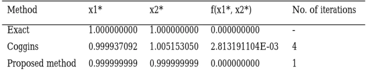
Table 5: Computational result for problem 5 (Rosenbrock’s function)
Method x1* x2* f(x1*, x2*) No. of iterations
Exact Coggins
Proposed method
1.000000000 0.999937092 0.999999999
1.000000000 1.005153050 0.999999999
0.000000000 2.813191104E-03 0.000000000
- 4 1
Table 6: Computational results for the problem 6
Method No. of iterations when n = 4 No. of iterations when n = 12
Fletcher-Reeves 11 15
Coggins 9 13
Proposed method 2 3
Table 7: Computational results for the problem 7 when n = 460
Method Average no. of iterations Success ratio
Fletcher-Reeves 620 420/1000
Coggins 310 820/1000
DISCUSSION OF RESULTS
The stopping criteria for problems 1 to 6 is. For the Fletcher-Reeves method, Armijo line search was used. From tables 1-7, the proposed method shows better performance with 99% success (by success we mean the num-ber of successful runs out of 1000 runs) in problem 7 and with clearly minimum num-ber of function evaluations resulting in a faster running. The problems were run us-ing Matlab 6.5 on HP Compact nx7300 lap-top. The execution time for the new method is in general about 78% faster than the execution time for Coggins method of 4]. From these results, the new Coggins – Fibonacci method is shown to be consis-tently very accurate and comparable with other methods. In particular, the present method converges faster than Coggins or Fibonacci method.
Our computational experience in this work, as highlighted in section 1, supports the as-sertion that the efficiency of an optimiza-tion method depends on the search direc-tion explored [20].
CONCLUSION
The Coggins – Fibonacci algorithm for solving n – dimensional (n≥1)
uncon-strained optimization problems is here pro-posed. The method is amenable to the usual mathematical analysis. By means of some test problems, the Coggins –Fibonacci method is shown to be no less inferior to other known methods for the rate of con-vergence is faster than most other methods.
REFERENCES
Adby, P.R., Dempster, M.A.H. 1974. In-troduction to optimization method. Chapman &
9 i 1
i
10 *) x ( f *) x (
f
Hall, London.
Agusto, F.B. 2002. Multivariable Coggins method. M.Sc. Thesis, University of Ilorin,
Ilorin, Nigeria.
Armijo, L. 1966. Minimization of function having Lipschitz continuous first partial de-rivatives. Pacific Journal of Mathematics, 16: 1-3. Bamigbola, O.M., Agusto, F.B. 2004. Op-timization in Ân by Coggins method.
Interna-tional Journal of Computer Mathematics, 81(9):
1145-1152.
Bunday, B.D. 1984. Basic optimization meth-ods. Edward Arnold, London.
Foulds, L.R. 1981. Optimization techniques. Springer-Verlag, New York.
Haykij, S. 1994. Neural networks: A comprehen-sive foundation. Macmillan college publishing
company, New York (NY).
Ibiejugba, M.A., Adewale, T.A., Bamig-bola, O.M. 1991. A Quasi-Newton method for minimizing factorable functions. Afrika
mathematika, 4(2): 19–36.
Kahya, E. 2006. Comment on titled “An improvement on Fibonacci search method in optimization theory. Applied mathematics and
computation, 176: 753-756.
Kuester, J.L., Mize, J.H. 1973. Optimization techniques with Fortran. McGraw-Hill, New
York.
Magoulas, G.D., Vrahatis, M.N., Andou-lakis, G.S. 1997. Effective backpropagation training with variable stepsize. Neural
net-works, 10: 69-82.
Subramaniam, S. 1994. Extended Coggins optimization techniques. B. Tech. Thesis,
De-partment of Mathematics, Computer Science and Statistics, Federal University of Technol-ogy, Minna, Nigeria.
Subramaniam, S., Reju, S.A., Ibiejugba, M.A. 2002. An extended Coggins optimiza-tion method. Nigeria Journal of Mathematics and
Applications, 8: 85-91.
Wallstreetcosmos.com, 2008. Fibonacci num-bers and stock market analysis. Downloaded on
March 14th, 2009.
Walsh, G.R. 1985. Methods of optimization. John Wiley & Sons, London.
More, B.J., Garbow, B.S., Hillstrom, K.E. 1981. Testing unconstrained optimiza-tion. ACM Transactions on Mathematical
Soft-ware, 7: 17-41.
Rao, S.S. 1991. Optimization theory and appli-cation, Eastern John Wiley, New Delhi. Reju, S.A. 2001. Roc-CMAI lecture notes. Na-tional Mathematical Centre, Abuja, Nigeria. Sperduti, A., Starita, A. 1993. Speed up learning and network optimization with ex-tended back-propagation. Neural networks, 6: 365-383.
Subasi, M., Yildirim, B., Yildiz, B. 2004. An improvement on Fibonacci search method in optimization theory. Applied
mathematics and computation, 147(3): 893-901.