Vol. 19, No. 01, pp 39-57 DOI:10.29252/jirss.19.1.39
Bounds for CDFs of Order Statistics Arising from INID Random
Variables
Jaber Kazempoor1, Arezou Habibirad1, and Kheirolah Okhli1
1Department of Statistics, Faculty of Mathematical Sciences, Ferdowsi University of Mashhad,
Mashhad, Iran.
Received: 26/03/2019, Revision received: 22/12/2019, Published online: 23/01/2020
Abstract. In recent decades, studying order statistics arising from independent and not necessary identically distributed (INID) random variables has been a remarkable concern for researchers. The cumulative distribution function (CDF) of these random
variables (Fi:n) is a complex manipulating, long time consuming and a
software-intensive tool that takes considerable time. Therefore, obtain approximations and
bounds forFi:n and other theoretical properties of these variables, such as moments,
quantiles, characteristic functions, and some related probabilities, has always been the main challenge. Recently, Bayramoglu (2018), Bayramoglu (2018), has introduced
a set of CDFs (F[i]), whose definitions are based on a point to point ordering of the
original CDFs (Fi), that can be used to approximate the CDF of i-th order statistics
(Fi:n). Here, by using justF[1] andF[n], we provide new upper and lower bounds for
theFi:n. Furthermore, new approximations forF1:nandFn:n, as well as for other cases,
are derived. Comparisons with respect to approximations suggested by Bayramoglu Bayramoglu (2018) are also provided.
Keywords. Approximation, Bounds, Cumulative Distribution Function, Independent and not Necessary Identically Distributed, Order Statistics.
Jaber Kazempoor ([email protected] )
Corresponding Author: Arezou Habibirad ([email protected]) Kheirolah Okhli ([email protected] )
MSC:62E17, 62E99, 62G07.
1
Introduction
Order statistics play a significant role in the mathematical statistics and other disciplines like in issues such as the investigation of natural disasters, the lifespan of a coherent system, extreme values, records, time series, discussion about the range of variables, and so forth. In all of the mentioned cases, we have to use the functions of a variety of ordered statistics. Order statistics arising from independent and identically distributed (IID) random variables have been studied in many sources, such as Ahsanullah et
al. (2013), Arnold et al. (1992), and David and Nagaraja (2004), but in some
situations, we must assess the behavior of order statistics arising from independent and not necessary identically distributed (INID) random variables. In this case, some theoretical properties, such as relations and formulas quickly became complicated and overwhelming (see David and Nagaraja (2004) and Reiss (2012)). However, many improvements have been made in the theoretical part of these cases, and although many formulas have a closed form in these situations, they are tedious and time consuming to deal with. Hence, these formulas cannot be applied in practice due to the complexity of the calculations and ample time consumption. Because of the mentioned reasons, many scholars have sought to approximate these relationships, build bounds for them, or compute them through the recurrence relationships in INID case as well as in IID (see Reiss (2012), Balakrishnan and Sultan (1998), Arnold and Balakrishnan (2012), and Balakrishnan et al. (1992)).
Now, consider INID random variables X1, . . . ,Xn with corresponding absolutely
continuous CDFs F1, . . . ,Fn. Denote by X1:n ≤ X2:n ≤ · · · ≤ Xn:n the order statistics
constructed from X1, . . . ,Xn. The CDF of rth order statistics Xr:n is (see David and
Nagaraja (2004))
Fr:n = P(Xr:n≤x)
= 1
r!(n−r)! n X
i=r X
S k Y
j=1
Ftj(x)
n Y
j=k+1 ¯ Ftj(x),
where the summationSextends over alln! permutationst1, . . . ,tnof 1, . . . ,n.
Given a set of INID variables Bayramoglu Bayramoglu (2018) defined the D-order
functions (F[i]) based on point to point ordering of given CDFs (Fi). He discussed
some useful properties of these definitions and showed that the corresponding random variables are independent. Finally, he suggested that these new functions could be used
as an alternative or an approximation of the order statistics CDFs (Fi:n).
His new definition of D-order functions is as follows:
First, consider INID random variablesX1,X2, . . . ,Xnwith, respectively,
correspondi-ng CDFsF1,F2, . . . ,Fn, and next suppose thatai = in f{x : Fi(x) >0} and bi = sup{x :
Fi(x) <1}. Then, therth D-order functionF[r](x), x ∈(a,b), 1 ≤r ≤n, wherea =aiand
b=bi(i.e., all CDFs have the same support) is defined asF[r](x) =Fj(x), if x∈Drjsuch
that
Drj={x:x∈[a,b],Fi
1(x)≥Fi2(x)≥ · · · ≥Fir−1(x)≥Fij(x)≥Fir+1(x)≥. . .Fin(x)},
for all
(i1,i2, . . . ,ir−1,ij,ir+1,in)∈Πj,r(1,2, . . . ,n),ik, j f or k,r,
whereΠj,r (1,2, . . . ,n) is the class of all sequences of lengthn, in which the rth place
is occupied by j, and the remaining (n−1) places are occupied by the elements of
possible (n−1)! permutations of numbers 1,2, . . . ,j−1,j+1, . . . ,n. In addition, for
the heterogeneous random domains, it is clear that without loss of generality, we can
extend this condition by definingaandbasa=min(ai) andb=min(bi), respectively.
The rest of the paper is organized as follows. We use only F[1] and F[n] for
constructing an improved approximations ofF1:nandFn:nand provide lower and upper
bounds forFr:nin Section 2. Unfortunately, these bounds are not CDFs, in the general
case, but they have very important and useful features, which means that they are not uniform and sensitive to the given values and vary in terms of changing the domain points of the bound functions. Moreover, these features are described extensively and relatively, and the corresponding formulas for the most of the theoretical properties of these order statistics, such as moments and the mathematical expectations, are presented.
In Section 3, we compare our approximation ofF1:nandFn:nwith the approximation
that is presented in Bayramoglu Bayramoglu (2018), and our approximation superiority will also be clearly represented throughout the figures. We also show, by another example, that even the bounds obtained in this study, work better than the D-order functions in many places.
2
Lower Bound, Upper Bound, and Approximation for
F
i:nin
INID Case
In this section, we find the lower and upper bounds for the CDFs of order statistics in INID case. Some of their important properties are discussed. We also provide a proper
approximation ofFi:nutilizing these bounds.
Following two definitions of the first and the last of D-order functions (F[1](x) and
F[n](x)), it is clear that
F[n](x)≤Fi(x)≤F[1](x),
and
¯
F[1](x)≤F¯i(x)≤F¯
[n](x).
These bounds motivate us to construct new bounds forF1:n(x) andFn:n(x) as
1−
n Y
i=1
¯
F[1](x)≤F1:n(x)=1− n Y
i=1
¯
Fi(x)≤1− n Y
i=1
¯ F[n](x),
and
n Y
i=1
F[n](x)≤Fn:n(x)= n Y
i=1
Fi(x)≤ n Y
i=1
F[1](x),
or equivalently
G1:n;[1](x)≤F1:n(x)≤G1:n;[n](x),
and
Gn:n;[n](x)≤Fn:n(x)≤Gn:n;[1](x),
whereGi:j;[k](x) (1≤i≤ j≤n, k =1,n) denote the CDFs ofith smallest order statistics
arising from j, IID random variables with the same CDF F[k](x). Note that, because
each of the presented bound alone is a CDF, we approximateF1:nandFn:n, as
F(1)(x)=
G1:n;[1](x)+G1:n;[n](x)
2 , (2.1)
F(n)(x)=
Gn:n;[1](x)+Gn:n;[n](x)
2 . (2.2)
The functions (2.1), and (2.2) are CDF, which we can use them for approximating
F1:nandFn:n,. In these approximations after utilizingGi:j;[k](x), we can use the strong
condition IID instead of the weaker condition INID.
Similar to the preceding Theorem, we construct bounds forFi:n,i=1, . . . ,n.
Theorem 2.1. If X1, . . . ,Xn are INID random variables with CDFs F1, . . . ,Fn, respectively,
then, for all 1≤i≤n,
LFi:n(x)≤Fi:n(x)≤UFi:n(x), (2.3)
where
LFi:n(x)=max n X
k=i n k !
Fk[n](x) ¯Fn[1]−k(x),1− i−1
X
k=0 n k !
Fk[1](x) ¯Fn[n−]k(x) , (2.4) and
UFi:n(x)=min n X
k=i n k !
Fk[1](x) ¯Fn[n−]k(x),1− i−1
X
k=0 n k !
Fk[n](x) ¯Fn[1]−k(x) . (2.5)
Proof. Consider, fori=0,1, . . . ,n,
Pi(x)=P(exactly i of X1, . . . ,Xn are≤x). Thus
n i !
F[in](x) ¯F[1]n−i(x)≤Pi(x)≤ n i !
Fi[1](x) ¯Fn[n−]i(x).
Now, apply the following formula (see Bairamov and Tavangar (2015)) Fi:n(x)=
n X
k=i
pk(x)=1− i−1
X
k=0 pk(x). Then, we get
n X
k=i n k !
F[kn](x) ¯F[1]n−k(x)≤Fi:n(x)≤ n X
k=i n k !
Fk[1](x) ¯Fn[n−]k(x), and
1−
i−1
X
k=0 n k !
F[1]k (x) ¯Fn[n−]k(x)≤Fi:n(x)≤1− i−1
X
k=0 n k !
Fk[n](x) ¯Fn[1]−k(x).
Finally, take minimum from upper bounds and maximum from lower bounds, to
complete the proof.
TheLFi:n(x) andUFi:n(x) have some interesting properties, which are listed below.
Bounds Properties :
• One of the important advantages of these bounds is the point to point dependence
to the fixed given value x, which means that LFi:n(x0), and UFi:n(x0) have the
different form ofLFi:n(x1) andUFi:n(x1), respectively, wherex0 ,x1. This property
makes the bounds functions flexible and causes the difference between the main
function and the related bounds as small as possible. Moreover, these bounds enable us to find a rigorous and tight confidence interval for many of the theoretical
properties ofXi:n, which are directly related to theFi:n, such as bounds for moment
generating functions, characteristic functions, and so on.
• It is obvious that the approximation of theFi:nin INID case, must also be satisfied
in the IID situations. Therefore, it is logical to expect that the alternative ofFi:n
in the INID case satisfies also the IID samples. However, it is easy to check that
F[i] ,Fi:nin the INID case as well as in the IID form. It is shown that our bound
and consequently our approximations ofFi:nbecomes equality for the IID case.
Proposition 2.1. Let X1, . . . ,Xnbe IID random variables with the same CDFs F; then
for all 1≤i≤n,
LFi:n(x) = UFi:n(x)
=
n X
k=i n k !
Fk(x) ¯Fn−k(x).
Proof. In the IID case, it is straightforward to check thatF[i] =F, and due to the
relationF+F¯ =1, we have
i−1
X
k=0 n k !
Fk[n](x) ¯Fn[1]−k(x)+ n X
k=i n k !
Fk[1](x) ¯Fn[n−]k(x)
=
i−1
X
k=0 n k !
Fk[1](x) ¯Fn[n−]k(x)+ n X
k=i n k !
Fk[n](x) ¯Fn[1]−k(x)
=
i−1
X
k=0 n k !
Fk(x) ¯Fn−k(x)+ n X
k=i n k !
Fk(x) ¯Fn−k(x)
=
n X
k=0
n k !
Fk(x) ¯Fn−k(x)=1.
Finally, with some slight calculations, the proof is completed.
• Since we are looking for an alternative representation of a CDF, it can be rational
to expect that our formula must have the CDF properties and consequently also our bounds too. According to the flexibility of these bounds, it is reasonable that we expect their first and last values are 0 and 1, respectively. In the following, we prove the accuracy of this statement. The continuousness of these bounds is clear, and only it is remained to check the increasing behavior of these bounds to
show the CDF feature ofLFi:n(x) andUFi:n(x). It is easy to achieve these properties
by plotting all bounds, so if these bounds are CDF, we can use a convex linear combinations of these functions or alternatively as a special case, its average as
a supersede of Fi:n. Otherwise, we can use one of these bounds (preferred one,
which is CDF) as an approximation.
Proposition 2.2. If X1, X2, . . . ,Xn are random variables, respectively, supported in [a1,b1], . . . ,[an,bn], ai,bi∈R,i∈N, and also relations(2.4)and(2.5)hold, then
LFi:n(a) = UFi:n(a)=0, LFi:n(b) = UFi:n(b)=1, where a=min(a1,a2, . . . ,an)and b=max(b1,b2, . . . ,bn). Proof. The CDF property of D-order functions results in
F[1](a)=F[n](a)=1−F[1](b)=1−F[n](b)=0.
On the other hand, fory={a,b},
F[1]i (y) ¯Fn[n−]i(y)=Fi[n](y) ¯F[1]n−i(y)=Ii=0(i)Iy=a(y)+Ii=n(i)Iy=b(y), where
Ii=0(i)= (
1 if i=0,
0 if i,0.
Now, it is obvious to see that, for alli=0,1, . . . ,n, n
X
k=i n k !
Fk[1](y) ¯Fn[n−]k(y) = n X
k=i n k !
Fk[n](y) ¯Fn[1]−k(y)
= Ii=0(i)Iy=a(y)+Ii=n(i)Iy=b(y).
Finally, with a little accuracy in relations (2.4) and (2.5) and some routine
mathem-atical calculations, the proof is completed.
• It is difficult to calculate all of the proposed CDFs by Bayramoglu, Bayramoglu
(2018), and frequently time-consuming, especially when the sample size is large. But in this strategy, we only need the first and the last of D-order functions. These two functions can be easily calculated in R statistical software Team (2018),
by two famous commands pmin and pmax, respectively, and the difficulty of
derivation Bayramoglu’s CDFs will be fixed. These features can increase the accuracy of the calculation and considerably reduce the time it takes to perform the calculation. Moreover, when the sample size becomes larger and larger, the
CDFs of extreme values tend more and more to the horizontal axis (Y = 0 and
Y = 1), and consequently, the precision of corresponding D-order alternatives
for these random variables becomes smaller and smaller. Because in D-order
approximations, the effect of sample size is nearly ignored, low accuracy results
when one wants to approximate the CDF of order statistics for large sample sizes.
• As the last lack of D-order functions, it is possible to mention their inattention
in approximation CDF of order statistics in the case that there exist some similar
CDFs amog the original CDFs. In an analytical form, assume n independent
random variables X1,X2, . . . ,Xn such that Xkj−1+1,Xkj, . . . ,Xkj ∼ Fj, where j =
1,2, . . . ,m andk0 = 0,Pmj=1kj = n. In this situation, there exist just m kinds of
D-order function aiming to approximatendifferent CDFs of order statistics. The
worst situation has occurred in the IID case since there is just one type of D-order
functions for approximationnkinds of CDFs of order statistics. Finally, it is worth
noting that our approximations fixed this problem as well as previous problems.
3
Examples
1 In this section, we provide two examples, which are an excellent showcases for
the previous theoretical backgrounds. The first example compares our result with Bayramoglu’s upshots. The second example represents the biasedness of D-order
functions forn=4 in comparison with our alternative representation.
Examples 3.1(Bayramoglu 2018, Bayramoglu (2018)). LetX1andX2be INID random
variables supported in [0,1], respectively, with corresponding CDFs F1(x) = (2x−x2)2, 0≤x≤1,
F2(x) = x, 0≤x≤1.
Then
F[1](x)=
(
x if 0≤x≤c,
(2x−x2)2 if c≤x≤1, F[2](x)=
(
(2x−x2)2 if 0≤x≤c,
x if c≤x≤1,
wherec= 3−
√ 5 2 .
Now, we approximateF1:2(x). According to relation (2.1), we have
F(1)(x) =
G1:2;[2](x)+G1:2;[1](x)
2
= 1−(1−F[2](x))2+1−(1−F[1](x))2
2
= (2x−x2)2+x−(2x−x
2)4+x2
2 ,
and similarly by relation (2.2), we obtain F(2)(x) =
G2:2;[2](x)+G2:2;[1](x)
2
= F
2
[1](x)+F2[2](x)
2
1In this part, all of the numerical calculation with 7 digits of decimals and drawing all graphs are done
with R statistical software; Team (2018).
= (2x−x2)4+x2
2 .
Our first step is to compare these approximations with the one provided by Bayram-oglu, Bayramoglu (2018). This comparison is shown in Figure 1. The accuracy of our approximation is clear, and also the adaptation of our results and the original function is surprising. This feature is because of the sensitivity of the bounds and its relative symmetry with respect to the original function. In fact, by using just two CDFs defined according to the D-order notion, we are able to improve the Bayramoglu’s presentations
forF1:2(x) andF2:2(x) with high accuracy. This note shows the importance of D-order
definitions.
0.0 0.2 0.4 0.6 0.8 1.0
0.0
0.2
0.4
0.6
0.8
1.0
Domain of random variables
CDFs of order statistics and their alter
nativ
es
F1:2 F[1] F(1) F2:2 F[2] F(2)
Figure 1: F1:2(x) andF2:2(x) and their alternatives
The next step is to calculate and display the bounds of F1:2(x) and F2:2(x). With
respect to Theorem 2.1, bounds may be CDFs or not. When, their mean is not a CDF,
we can not use the mean of two bounds as an approximation ofFi:n. It has two benefits.
Firstly, it provides additional information about our bounds, which those of them are
CDF or not. Secondly, it can well evaluate the range of occurrence of many probabilities.
Besides, we can consider lower and upper bounds ofR h(x)dFi:n(x) for any monotone
functionh(.). This feature also can enable us to construct bounds for some theoretical
properties of any ordinary order statistics arising from INID random variables such as moment generating function and moments for nonnegative and negative random variables.
By Theorem 2.1, we can find bounds forF1:2(x),
maxn1−F¯2
[2](x),2F[2](x) ¯F[1](x)+F2[2](x) o
≤F1:2≤minn1−F¯2
[1](x),2F[1](x) ¯F[2](x)+F2[1](x) o
,
and similarly, forF2:2,
maxnF2[2](x),1−F¯2
[2](x)−2F[1](x) ¯F[2](x) o
≤F2:2≤minnF2
[1](x),1−F¯2[1](x)−2F[2](x) ¯F[1](x) o
.
In Figure 2, the bounds ofF1:2(x) andF2:2(x) are shown.
0.0 0.2 0.4 0.6 0.8 1.0
0.0
0.2
0.4
0.6
0.8
1.0
Domain of random variables
CDFs and bounds f
or order statistics
F1:2 LF1:2 UF1:2 F2:2 LF2:2 UF2:2
Figure 2: F1:2(x) andF2:2(x) and their bounds
The goodness of these bounds can be immediately understood, which means that
depending on any given value, these bounds also have different values and are not
uniformly bounded.
Based on Figure 2, it is evident that the bounds are itself CDFs and in each case, we can utilize the mean of two bounds as an approximation of order statistics CDFs as we previously have done. For more understanding of the performance of these bounds, we compare them with D-order functions. This comparison is depicted in Figure 3.
It is clear that the upper bound ofF1:2and the lower bound ofF2:2are much better
alternatives forF1:2(x) andF2:2(x) in comprised with the corresponding approximations
of Bayramoglu’sF(1)(x) andF(2)(x). Even the performance of the lower bound ofF1:2
and the upper bound ofF2:2in the dominated part of the random variable domains are
better than the corresponding approximations of D-order functions. (By approximating
the CDFs of order statistics, it is clear, that our approximation all over the interval [0,1],
are significantly closed to the original functions as it can be seen in Figure 3. It is
noteworthy that, the performances ofLF1:2(x) andUF2:2(x) is better than Bayramoglu’s
presentation, in the intervals [0.152,1] and [0,0.718] respectively, which means these
bounds are better than Bayramoglu’s approximation in 85 and 71 percent of situations.) This proposition itself can show the importance of these bounds, and there is even a
reason to use these functions as an approximation ofF1:2(x) andF2:2(x).
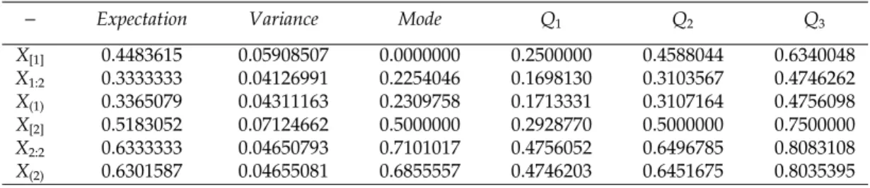
Finally, F(1) andF(2) are CDFs, hence there exist corresponding random variables
X(1)andX(2), respectively. It is interesting to compare the expected values, variance, the
first quartile (Q1), median (Q2), and the third quartile (Q3) of these random variables
with what calculated through D-order functions.
These measures can be found in Table 1. Based on this table, one can see the closeness
of all tendency measures ofXi:2andX(i).
Table 1: Measures of central and skewed tendency for presented random variables
− Expectation Variance Mode Q1 Q2 Q3
X[1] 0.4483615 0.05908507 0.0000000 0.2500000 0.4588044 0.6340048
X1:2 0.3333333 0.04126991 0.2254046 0.1698130 0.3103567 0.4746262
X(1) 0.3365079 0.04311163 0.2309758 0.1713331 0.3107164 0.4756098
X[2] 0.5183052 0.07124662 0.5000000 0.2928770 0.5000000 0.7500000
X2:2 0.6333333 0.04650793 0.7101017 0.4756052 0.6496785 0.8083108
X(2) 0.6301587 0.04655081 0.6855557 0.4746203 0.6451675 0.8035395
0.0 0.2 0.4 0.6 0.8 1.0
0.0
0.2
0.4
0.6
0.8
1.0
Domain of random variables
D−order functions and CDFs f
or order statistics and their bounds
F1:2 F[1] LF1:2 UF1:2 F2:2 F[2] LF2:2 UF2:2
Figure 3: F1:2(x) andF2:2(x), their bounds and D-order functions
This example can be considered as a special case of the following Lemma.
Lemma 3.1. Let F1and F2be two CDFs with the same supported interval such that the equation
F1(x)−F2(x)=0has at most three different real solutions. Then
F(1)(x) = F1(x)+F2(x)−
F2
1(x)+F22(x)
2 ,
F(2)(x) =
F21(x)+F22(x)
2 ,
Fr(1)(x)+Fr(2)(x) = Fr1(x)+Fr2(x), r∈R, Fr(1)(x)×Fr
(2)(x) = F
r
1(x)×F
r
2(x), r∈R,
f(1)(x)+ f(2)(x) = f1(x)+ f2(x),
µr
(1)(x)+µ
r
(2)(x) = µ
r
1(x)+µ
r
2(x), r∈R,
provided that the expectations exist.
Proof. Two obvious solutions are the first and the last point of the given interval, and in this case it is obvious to see thatF[1](x)=max{F1(x),F2(x)}andF[2](x)=min{F1(x),F2(x)}.
Consequently, for any functiong(.), we have
g(F[2](x))+g(F[1](x))=g(F1(x))+g(F2(x)), (3.1)
and
g(F[2](x))g(F[1](x))=g(F1(x))g(F2(x)). (3.2)
Finally letg(x)=1−(1−x)2andg(x)=x2, in relations (2.1) and (2.2), to complete the
proof in this case.
In another case, we have an extra real solution in the interval, sayc, and
F[1](x)=
(
F1(x) if x≤c,
F2(x) if c≤x, F[2](x)=
(
F2(x) if x≤c,
F1(x) if c≤x,
or
F[1](x)=
(
F2(x) if x≤c,
F1(x) if c≤x, F[2](x)=
(
F1(x) if x≤c,
F2(x) if c≤x;
Again it is straightforward to see that relations (3.1) and (3.2) hold for any function
g(.), as considered previously. Now, the proof is similar to the proof of the previous
case.
An interesting fact about this lemma is that forn= 2, we do not need to calculate
the Bayramolu’s CDFs and our approximations ofFi:ncan be easily derived from the
original CDFs. In addition, some theoretical properties of corresponding random variables such as moments and probability density functions can be calculated in the same manner.
Here, we present an example forn=4 to show the method of deriving alternatives
for CDF of any order statistics. Likewise, it can be observed that the tendency behavior of CDFs of extreme values approaches to the horizontal axis, and it leads to the bad performance of corresponding D-order functions.
Examples 3.2. Let X1, X2, X3, and X4 be INID random variables supported in [0,1],
respectively, which have CDFs
F1(x) = (2x−x2)2, 0≤x≤1,
F2(x) = x, 0≤x≤1,
F3(x) =
1−e−x
1−e−1, 0≤x≤1,
F4(x) = Φ
(x)−0.5
Φ(1)−0.5, 0≤x≤1,
whereΦ(x)=R−∞x √1
2πe −t2
2dt.
Then the D-order of these function are obtained as
F[1](x)=F1(x)I[0,0.6175849](x)+F3(x)I[0.6175849,1](x),
F[2](x)=F4(x)I[0,0.4966055](x)+F3(x)I[0.4966055,0.6175849](x)+F1(x)I[0.6175849,1](x),
F[3](x)=F2(x)I[0,0.3819655](x)+F3(x)I[0.3819655,0.4966055](x)+F4(x)I[0.4966055,1](x),
and
F[4](x)=F3(x)I[0,0.3819655](x)+F2(x)I[0.3819655,1](x),
where
IA(x)= (
1 if x∈A,
0 if o.w.
As previously proved, ifLFi:nandUFi:nare increasing functions, then they are also
CDF’s. Consequently, whenn>2, in the first step, all of the bound functions should be
drawn in order to determine which of them have a nondecreasing feature. Then, for any
fixedi, if both of corresponding bounds are nondecreasing, then we can approximate
Fi:n, by taking mean of these bounds, or any arbitrary convex linear combinations.
However, when one of the corresponding bounds do not have nondecreasing property, it is preferred to choose one bound function, which has a nondecreasing property as
an alternative representation for correspondingFi:n. Finally, if none of two bounds are
CDFs, we can only boundFi:nand another related theoretical property.
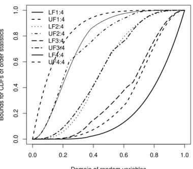
Now we have to examine if the bounds are CDFs or not. By drawing these bounds, it is clearly understood that all of them are CDFs. Nondecreasing property of all bounds
can be obviously seen in Figure 4, and consequently, we can approximate each ofFi:n.
These substitutes are the mean of two corresponded bounds.
0.0 0.2 0.4 0.6 0.8 1.0
0.0
0.2
0.4
0.6
0.8
1.0
Domain of random variables
Bounds f
or CDFs of order statistics
LF1:4 UF1:4 LF2:4 UF2:4 LF3:4 UF3:4 LF4:4 UF4:4
Figure 4: Lower and upper bounds for all CDFs of ordinary order statistics
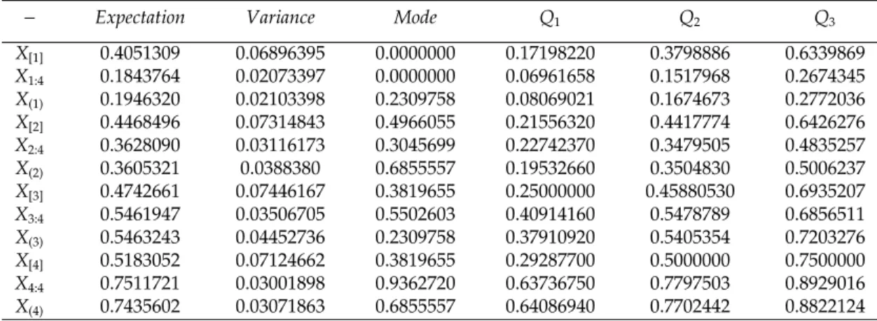
From another point of view, due to the fact that our approximations are also CDFs, there exist corresponding random variables, for which we are interested in comparing some of their measures of central and skewed tendency. Their moments are collected in Table 2.
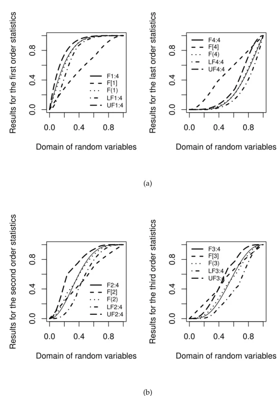
It is observed that for almost all of the provided measures, the accuracy of our results is much better than Bayramoglu’s alternatives. Moreover, our approximations, D-order corresponding functions, and upper and lower bounds for CDFs of ordinary order statistics arising from these heterogeneous random variables, are shown in Figures 5a and 5b. The comparison results for extreme values of this example (first and last ordinary order statistics) can be seen in Figure 5a. As mentioned in the first item of bounds properties, the performance of prime and latter D-order functions get worse and worse by increasing the sample size. This note can be clearly understood in this figure.
D-order functions performance is far better in the approximation of middle ordinary order statistics as seen in Figure 5b, but still it is unfavorable in comparison with our representations.
4
Conclusion and Recommendation
We considered INID random variablesX1, . . . ,Xnwith respectively CDFsF1, . . . ,Fnand
utilized the first and the last D-order functions to construct lower and upper bounds for
any CDF of ordinary order statistics (Fi:n). We proved all of the necessary and sufficient
conditions of these bounds to be a CDF except their nondecreasing behavior features. This property remains as an open problem for the researches to prove or contradict. This gap can be fixed by drawing all of the bounds with R statistical software (Team (2018)). The related command are also given in the text.
The new definition of D-order functions seems to be very appealing and therefore useful. Their main advantages are independence and the fact that they are CDFs. Unfortunately, when the sample size increases, the calculation of D-order functions becomes long and time-consuming. Furthermore, the performance of the first and the last of these functions get worse. Finally, the manner of fixing these deficiencies are widely expressed.
Table 2: Measures of central and skewed tendency of the random variables having CDFs described in Example 3.2.
− Expectation Variance Mode Q1 Q2 Q3
X[1] 0.4051309 0.06896395 0.0000000 0.17198220 0.3798886 0.6339869
X1:4 0.1843764 0.02073397 0.0000000 0.06961658 0.1517968 0.2674345
X(1) 0.1946320 0.02103398 0.2309758 0.08069021 0.1674673 0.2772036
X[2] 0.4468496 0.07314843 0.4966055 0.21556320 0.4417774 0.6426276
X2:4 0.3628090 0.03116173 0.3045699 0.22742370 0.3479505 0.4835257
X(2) 0.3605321 0.0388380 0.6855557 0.19532660 0.3504830 0.5006237
X[3] 0.4742661 0.07446167 0.3819655 0.25000000 0.45880530 0.6935207
X3:4 0.5461947 0.03506705 0.5502603 0.40914160 0.5478789 0.6856511
X(3) 0.5463243 0.04452736 0.2309758 0.37910920 0.5405354 0.7203276
X[4] 0.5183052 0.07124662 0.3819655 0.29287700 0.5000000 0.7500000
X4:4 0.7511721 0.03001898 0.9362720 0.63736750 0.7797503 0.8929016
X(4) 0.7435602 0.03071863 0.6855557 0.64086940 0.7702442 0.8822124
0.0 0.4 0.8
0.0
0.4
0.8
Domain of random variables
Results f
or the first order statistics
F1:4 F[1] F(1) LF1:4 UF1:4
0.0 0.4 0.8
0.0
0.4
0.8
Domain of random variables
Results f
or the last order statistics
F4:4 F[4] F(4) LF4:4 UF4:4
(a)
0.0 0.4 0.8
0.0
0.4
0.8
Domain of random variables
Results f
or the second order statistics
F2:4 F[2] F(2) LF2:4 UF2:4
0.0 0.4 0.8
0.0
0.4
0.8
Domain of random variables
Results f
or the third order statistics
F3:4 F[3] F(3) LF3:4 UF3:4
(b)
Figure 5: Comparison of different upshot for the middle order statistics
Acknowledgment
We wish to thank anonymous referees for their constructive comments, and Professor A .R. Nematollahi, as the editor for his careful reading and interesting suggestions on an earlier version of this paper which significantly improved the presentation and led to put many details.
References
Ahsanullah, M., Nevzorov, V. B., and Shakil, M. (2013), An introduction to order statistics.
Arnold, B. C. and Balakrishnan, N. (2012),Relations, bounds and approximations for order
statistics, Springer Science & Business Media, volume 53.
Arnold, B. C., Balakrishnan, N., and Nagaraja, H. N. (1992), A first course in order
statistics, volume 54, Siam.
Bairamov, I. and Tavangar, M. (2015), Residual lifetimes of k-out-of-n systems with
exchangeable components.Journal of The Iranian Statistical Society,14(1), 63–87.
Balakrishnan, N., Bendre, S., and Malik, H. (1992), General relations and identities for
order statistics from non-independent non-identical variables.Annals of the Institute
of Statistical Mathematics,44(1), 177–183.
Balakrishnan, N. and Sultan, K. (1998), 7 recurrence relations and identities for moments
of order statistics.Handbook of Statistics,16, 149–228.
Bayramoglu, I. (2018), A note on the ordering of distribution functions of inid random
variables.Journal of Computational and Applied Mathematics,343, 49–54.
David, H. A. and Nagaraja, H. N. (2004), Order statistics. Encyclopedia of Statistical
Sciences.
Reiss, R.-D. (2012), Approximate distributions of order statistics: with applications to
nonparametric statistics.Springer Science & Business Media.
Team, R. C. (2018), R: A language and environment for statistical computing.