Vol 60, No 2 (2017)

(1)

TECHNICAL UNIVERSITY OF CLUJ-NAPOCA

ACTA TECHNICA NAPOCENSIS

Series: Applied Mathematics, Mechanics, and Engineering Vol. 60, Issue II, June, 2017

MASS DISTRIBUTION IN ANALYTICAL DYNAMICS OF SYSTEMS

Iuliu NEGREAN

Abstract: In the case of the multibody systems (MBS), as example the mechanical robot structure, a few simplifying

hypotheses, referring to mass properties, are implemented. According to these, the mass properties are continuously distributed between the fixed basis and the last kinetic ensemble from mechanical structure. As a result, in the dynamical study of MBS, the author of the paper has introduced the phrase “mass distribution” instead of mass geometry, typically too rigid solid. Mass distribution is based on the mass as fundamental notions in analytical dynamics of systems. At its turn, mass together with energy highlight the matter notion. But, mass is also highlighted by means of the two properties: gravitation and inertia. According to fundamental theorems from Newtonian dynamics, in the case of the translation motion the inertia property is highlighted by mass and position of the mass center. In the case of the resultant rotation motion the inertia property is characterized by mechanical moments of inertia and extension of these properties, known as inertial tensors and pseudoinertial tensors. Their matrix expressions are compulsory included in the dynamical notions like: kinetic energy, acceleration energy, angular momentum and their time derivatives according to differential equations of higher order, typically to analytical dynamics of systems.

Key words: analytical dynamics, mechanics, mass distribution, dynamics equations.

1. INTRODUCTION

The multibody systems (MBS), and as result the mechanical robot structure, are characterized through the mass properties continuously distributed between the fixed basis and the last kinetic ensemble from mechanical structure [2] and [3]. Consequently, the author of the paper has introduced, in the dynamical study, the phrase “mass distribution” instead of mass geometry, typically too rigid body. Physically, mass distribution (MD) is based on the mass. At its turn, mass and energy highlight the matter notion. But, mass, as fundamental notion in analytical dynamics, is also highlighted by means of the two properties: gravitation and inertia. According to fundamental theorems from Newtonian dynamics, in the case of the translation motion the inertia is highlighted by mass and position of the mass center. In the case of the resultant rotation motion the inertia property is characterized by mechanical moments of inertia (Leonard Euler, 1758 year) and extension of these properties, known as inertial tensor and pseudoinertial tensor [2] and [8]. Their matrix expressions are compulsory

included in the dynamical notions like: angular momentum, kinetic energy, acceleration energy of higher order, as well as their time derivatives, according to differential equations of higher order, typically to analytical dynamics [1] - [9].

In this paper, using the author researches, the properties of mass distribution (MD – type) will be developed [2] - [8]. In view of this, a few simplifying hypotheses are compulsory applied. So, every kinetic ensemble, belonging to MBS, is considered a rigid body, see Fig.1.

Fig.1 Kinetic Ensemble from MBS

elementul i

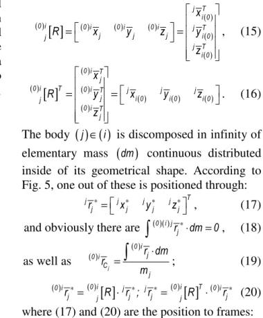
0

Ci

r 0

i i

r =p

i

C

i Ci

r

(

; i

)

i i

M I

{ }0 { }i

{i+1}

(2)

In the same time, MD – type properties are based on mass and geometrical integrals. These can be applied, in exclusivity, in the case of the homogeneous bodies with a simple or regular geometrical shape. But, any homogeneous body is characterized by the constant density in the infinity of elementary mass

₍

dm

₎

continuous distributed inside of its geometrical shape:

{

V A L

}

dm= ρ ⋅dV ;ρ ⋅dA ; ρ ⋅dL . (1) According to set (1), mass

₍

dm

₎

and density are functions of geometry of the homogeneous body. Usually, every kinetic ensemble is a compound body with non-regular geometrical shape, for which mass integrals cannot be applied. As example, the kinetic ensemble i= →1 n (Fig. 1) belonging to MBS is considered. Its geometrical shape shows as Fig. 2 and Fig.3.

Fig.2 Kinetic Ensemble

C1

xiG

OiG

li

ziG

yiG

C4

C3

C2

C5

C6

a1

z1

y1

x1

z2

y2

x2

z3

y3

x3

z4

y4

x4

x6

x5

z5

y6

z6

y5

4 ₂

1 3

6 5

Fig.3 Kinetic Ensemble discomposed

As a result of the above aspects, every kinetic ensemble i= →1 n is discomposed in a finite number of homogeneous bodies with a simple or regular geometrical shape, symbolized:

( ) ( )

j ∈ i , j= →1 p_i, and p_i∈N ( natural numbers ).

On the basis of the above considerations and the formulations of the author, in this paper the MD – type properties will be develop: mass and position of the mass center, mechanical moments of inertia (axial, planar, polar and centrifugal moments of inertia), inertial tensor and its generalized variation law, pseudo inertial tensor, as well as the algorithm of the mass properties corresponding to MBS. Among of these, inertial tensor is a squared matrix of the mechanical moments of inertia, while the pseudoinertial tensor is a squared matrix of mass moments of zero, first and second order [2].

2. MASS. POSITION of MASS CENTER

Considering the geometrical and mass aspects from the first section, for define mass and position of the mass center corresponding to a kinetic ensemblei= →1 n, in the first step this is divided inj= →1 p_i homogeneous body

( ) ( )

j ∈ i with a simple geometrical shape [2].

So, for beginning mass and position of the mass center is determined for every homogeneous

body

_{( ) ( )}

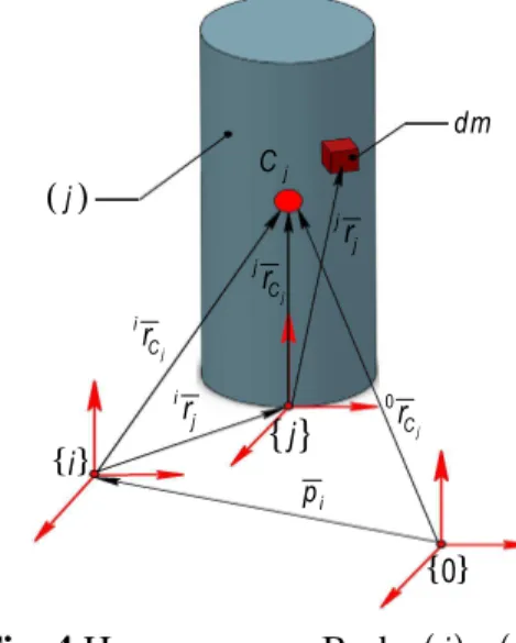
j ∈ i , represented as example in Fig. 4.

Fig. 4 Homogeneous Body

( ) ( )

j ∈ i

To this body is attached a Cartesian frame

{ }

j , and then is discomposed in infinity of elementary mass

₍

dm

₎

continuous distributed inside of its geometrical shape. One out of these is positioned throughjrj . The total mass is:

j

m =

∫

dm; (2) where

₍

dm

₎

is substituted by (1) in function of geometry of the body. According to [2] and [4], the position of the mass center is defined with:

j

j j j

C

j r dm r

m ⋅

=

∫

. (3) But, the position of the mass center C_j must be determined to frames

_{{ }}

i or

_{{ }}

0 corresponding to kinematical structure of MBS. As a result, the expressions are written below as follows:

( ) ( ) ( )

[ ]

j j

0 i

0 i 0 i j

C j j C

r = r + R ⋅ r ; (4)

( )

[ ]

j

0 i j

0 i _C

C j

r r

T 1 1

   

= ⋅

   

   

  ; (5)

j

C

dm

( )j

{ }0

i

p

{ }j { }i

j

i C r

i j

r 0

j

C r j

j r j

(3)

where sometimes

{ }

j _OR ≡

{ }

i _OR is recommended. According to [2], the symbol:( )0 i_j

[ ]

R and ( )0 i_j

[ ]

T expresses the rotation and respectively locating matrix between frames

{ }

j and

{ }

i or

{ }

0 (Fig.4). When the above expressions (2), (3), (4) or (5) are applied for all bodiesj= →1 p_i, then mass and position of the mass center of the kinetic ensemblei= →1 n will be determined below as:

i

p

i j j

j 1

M σ m

=

∑

⋅ , (6)

where σ_j =

{

₍

1, j∈i ; 0; j

_{) (}

∉i

₎

}

; (7)

( )

i

j i

p

0 i

j C j

j 1 0 i

C

i

r m

r

M

σ =

⋅ ⋅

=

∑

, (8)

[ ]

i i

0 i

0

C C

i

r r

T

1 1

   

= ⋅

   

   . (9)

Expression (6) is devoted to establishment the total mass of the kinetic ensemble, while (8) or (9) is corresponding to position of mass center.

3. INERTIAL TENSOR for RIGID BODY

When the kinetic ensemblei= →1 n, from MBS, is characterized by the resultant rotation motion, then the inertia property is highlighted by mechanical moments of inertia and extension of these properties, known as inertial tensor and pseudoinertial tensor [2] - [4]. Similarly with the previous section, for beginning the above inertia properties will be determined in the case to every homogeneous body

_{( ) ( )}

j ∈ i , example Fig.5.

Fig. 5 Homogeneous Body

( ) ( )

j ∈ i

Every homogeneous body

( ) ( )

j ∈ i was analyzed from view point of the mass (2) and position of the mass center (3), (4) or (5). As a result, mass

j

m and mass center C_j are well defined. In keeping with Fig.5, mass center C_j is the origin for three concurrent frames, below presented:

{ }

{

}

j _OR OR _OR OR

C ∈ j ; i∗ ≡ i ; 0∗ ≡ 0 . (10)

Considering the formulations of the author, a few symbols and notations are implemented:

{

}

{

}

{

}

j j j j j j j j j j j j

u = x ; y ; z ; v = y ; z ; x ; w = z ; x ; y (11)

( )

_{

( ) ( ) ( )

_}

( )

{

( ) ( ) ( )

}

0 i 0 i 0 i 0 i

j j j j

i 0 i 0 i 0 i 0

u x ; y ; z

u x ; y ; z

 ₌ 

 

 

=

 

 

, (12)

( )

{

( ) ( ) ( )

}

( )

{

( ) ( ) ( )

}

0 i 0 i 0 i 0 i

j j j j

i 0 i 0 i 0 i 0

v y ; z ; x

v y ; z ; x

 ₌ 

 

 

=

 

 

, (13)

( )

_{

( ) ( ) ( )

_}

( )

{

( ) ( ) ( )

}

0 i 0 i 0 i 0 i

j j j j

i 0 i 0 i 0 i 0

w z ; x ; y

w z ; x ; y

 ₌ 

 

 

=

 

 

; (14)

where (11) are Cartesian coordinates or axes, while (12), (13) and (14) are the unit vectors between frames

_{{ }}

j and

_{{ }}

i or

_{{ }}

0 , respectively

between

_{{ }}

i or

_{{ }}

0 and

_{{ }}

j . On the basis of the above notations, the rotation matrix is written:

( )

[ ]

( ) ( ) ( )

( )

j T i 0

0 i 0 i 0 i 0 i j T

j j j i 0

j

j T i 0 x

R x y z y

z

   

 

=_ _= 

     

, (15)

( )

[ ]

( )

( ) ( ) ( )

0 i T j

0 i T 0 i T j j j

j i 0 i 0 i 0

j

0 i T j x

R y x y z

z

   

 

= =_ _

     

. (16)

The body

( ) ( )

j ∈ i is discomposed in infinity of elementary mass

(

dm

)

continuous distributed inside of its geometrical shape. According to Fig. 5, one out of these is positioned through:

T

j j j j

r∗=_ x∗ y∗ z∗_ , (17) and obviously there are

∫

( )( )0 i jr_j∗⋅dm=0, (18)

as well as ( )

( )

j

0 i j 0 i

C

j r dm r

m ⋅

=

∫

; (19)

( ) ( )

[ ]

( )

[ ]

( )

0 i 0 i T

0 i j j 0 i

j _j j j _j j

r∗= R ⋅ r ; r∗ ∗ = R ⋅ r∗ (20) where (17) and (20) are the position to frames:

j

C

d m

( )j

{ }0

i

p

{ }j

{ }i

j

i C

r

i j

r

0

j

C

r

ju

δ∗

j j

r∗

0

j

r

0

j_u

{ }i∗

(4)

{ }

{ } { }

{

j ; i ; 0

}

Cj

∗ ∗ _∈ _.

Expression (20) is rewritten below as follows:

( )

0 i j T

j i 0

0 i j T j

j i 0 j

0 i j T

j i 0

x x

y y r

z z

∗

∗ ∗

∗

   

   

= ⋅

 

   

   

. (21)

Another notation, compulsory applied in this study, is the skew symmetric matrix associated to position vector (17), as well its transpose:

j j

j j j

j j

0 z y

r z 0 x

y x 0

∗ ∗

∗ ∗ ∗

∗ ∗

 ₋ 

 

 _{× =} _ ₋ _  

 

−

 

 

, (22)

T

j j

r∗ r∗

 _× _{= −} _×

   . (23)

Whereas the inertia properties must defined to

{ }

i or

_{{ }}

0 , elementary mass is also positioned as:

( ) ( ) ( )

[ ]

j

0 i

0 i 0 i j

j C _j j

r = r + R ⋅ r∗; (24)

( )

[ ]

( )

[ ]

( )

[ ]

₍ ₎

j

0 i 0 i

C

0 i j

j

1 3

R r

T

0 1

×

 

 

=_ _

 

, (25)

( )

[ ]

( )

[ ]

₍ ₎

( )

j

0 i T

j 3 1

0 i T

j _{0 i} _T

C

R 0

T

r 1

×

 

 

=_ _

 

 

, (26)

( ) _{( )}

[ ]

0 i j

0 i _j

j j

r

r _T

1 1

∗

   

= ⋅

     

  ; (27)

where (27) with (25) shows the position of elementary mass in homogeneous coordinates.

Since every homogeneous body

_{( ) ( )}

j ∈ i is considered with simple geometrical shape, the mass and geometrical integrals are applied as:

(

)

j j 2 j 2

u j j

j j j j j 2

uv j j uu j

I v w dm

I u v dm; I u dm

∗ ∗ ∗

∗ ∗ ∗ ∗ ∗

 ₌ ₊ _⋅ 

 

 

= ⋅ ⋅ = ⋅

 

 

∫

. (29)

So, axial, centrifugal and planar mechanical moments of inertia with respect to

_{{ }}

j ∈C_j are known, and they are included in the next set:

( ) ( )

{

j j j

}

u uv uu i

I ; I ; I ; where j∗ ∗ ∗ = →1 p ; j ∈ i . (30) Considering the author formulations, in the next step must be determined axial, centrifugal and planar mechanical moments of inertia with

respect to

{

{ } { }

i∗ ; 0∗

}

∈C_j, according to set:

( ) ( ) ( )

_{( ) ( )}

{

0 i 0 i 0 i

}

ju juv juu i

I ;∗ I∗ ; I∗ ; where j= →1 p ; j ∈ i (31)

The moment of inertia is a mass integral, [2] - [9]. It is applied on the product between mass

(

dm

)

and the squared distance to an axis or plane, thus:

( )

₍

( ) ( )

₎

( ) ( ) ( ) ( ) ( )

0 i 2 0 i 2 0 i 2

ju ju j j

0 i 0 i 0 i 0 i 0 i 2

juv j j juu j

I dm v w dm

I u v dm; I u dm

δ

∗ ∗ ∗ ∗

∗ ∗ ∗ ∗ ∗

 ₌ _⋅ ₌ ₊ _⋅ 

 

 

= ⋅ ⋅ = ⋅

 

 

∫

(32)

The distance from mass

₍

dm

₎

to an axis having

as unit vector ju_{i 0}_{( )} (see Fig. 5) is determined as:

( )

j j

ju ui 0 rj

δ∗ = × ∗ , (33)

( )

(

)

(

( )

)

( ) ( )

T

2 j j j j

ju i 0 j i 0 j

T

j T j j j

j j

i 0 i 0

u r u r

u r r u

δ∗ ∗ ∗

∗ ∗

 

= × ⋅ × =

 

 

   

 ₌ _⋅_ _{× ⋅}_{ } _×_ _⋅ 

 

. (34)

As a result, considering (32) and (34), axial mechanical moment of inertia is defined thus:

( )

{

}

( )

0 i 2

ju ju

T

j T j j j

j j

i 0 i 0

I dm

u r r dm u

δ

∗ ∗

 ₌ _⋅ ₌ 

 

 

   

= ⋅ × ⋅ × ⋅ ⋅

 _ _{ } _ 

 

∫

. (35)

But, the mechanical moments of inertia, from (32), can be obtained on basis of coordinates included in the transfer matrix expression (21):

( )

( ) ( )

( )

0 i j T j

j i 0 j

0 i j T j

j i 0 j

0 i j T j

j i 0 j

u u r

v v r

w w r

∗ ∗

 ₌ _⋅ 

 

= ⋅

 

 

= ⋅

 

 

; (36)

( )

( ) ( )

( )

( ) ( )

( )

( ) ( )

0 i 2 j T j j T j

j i 0 j j i 0

0 i 2 j T j j T j

j i 0 j j i 0

0 i 2 j T j j T j

j i 0 j j i 0

u u r r u

v v r r v

w w r r w

∗ ∗ ∗

 ₌ _⋅ _⋅ _⋅ 

 

= ⋅ ⋅ ⋅

 

 

= ⋅ ⋅ ⋅

 

 

. (37)

The squared distance from mass

₍

dm

₎

to the mass center C_j is characterized by expression:

( ) ( ) ( )

( ) ( )

0 i 2 0 i 2 0 i 2

j j j

0 i T 0 i j T j

j j j j

u v w

r r r r

∗ ∗ ∗

∗ ∗ ∗ ∗

 ₊ ₊ ₌ 

 

 

= ⋅ ≡ ⋅

 

 

. (38)

The matrix

(

3 3×

)

, from (37), is identical with: T

j j T j T j j j

j j j j 3 j j

r∗⋅ r∗ = r∗ ⋅ r∗⋅ −I _ r∗× ⋅ _{ } r∗×_ . (39) Substituting (39) in (37), expressions become:

( )

( ) ( )

0 i 2 j T j

j j j

T

j T j j j

j j

i 0 i 0

u r r

u r r u

∗ ∗ ∗

∗ ∗

 ₌ _⋅ ₋ 

 

 

   

− ⋅ × ⋅ × ⋅

 _ _{ } _ 

 

, (40)

( )

( ) ( )

0 i 2 j T j

j j j

T

j T j j j

j j

i 0 i 0

v r r

v r r v

∗ ∗ ∗

∗ ∗

 ₌ _⋅ ₋ 

 

 

   

− ⋅ × ⋅ × ⋅

 _ _{ } _ 

 

(5)

( )

( ) ( )

0 i 2 j T j

j j j

T

j T j j j

j j

i 0 i 0

w r r

w r r w

∗ ∗ ∗ ∗ ∗  ₌ _⋅ ₋          − ⋅ × ⋅ × ⋅  _ _{ } _   

; (42)

( ) ( ) ( ) ( ) ( )

( ) ( )

0 i 2 0 i 2 0 i T 0 i 0 i 2

j j j j j

T

j T j j j 2

j j ju

i 0 i 0

v w r r u

u r r u δ

∗ ∗ ∗ ∗ ∗ ∗ ∗ ∗  ₊ ₌ _⋅ ₋ ₌         = − ⋅ × ⋅ × ⋅ ≡  _ _{ } _    . (43)

Therefore, using either (34) or (43), the axial mechanical moment of inertia (35) is rewritten:

( )

{

}

( )

T

0 i j T j j j

ju i 0 j j i 0

I∗ = u ⋅

∫

_ r∗× ⋅_{ }  r∗×_ ⋅dm ⋅ u . (44) Mass integral from (35) or (44) is symbolized:

T

j j j

x xy xz

j j j

yx y yz

j j j

zx zy z

I r r dm

I I I

∗ ∗ ∗ ∗ ∗ ∗ ∗ ∗ ∗ ∗ ∗ ∗  _ _{ } _  = _ × ⋅_{ } ×_ ⋅ =     ₋ ₋         = − −         − −        

∫

, (45)

(

)

(

)

(

)

j j 2 j 2

x j j

j j 2 j 2

y j j

j j 2 j 2

z j j

I y z dm

I z x dm

I x y dm

∗ ∗ ∗ ∗ ∗ ∗ ∗ ∗ ∗  ₌ ₊ _⋅      = + ⋅     = + ⋅    

∫

, (46)

j j j

xy j j

j j j

yz j j

j j j

zx j j

I x y dm

I y z dm

I z x dm

∗ ∗ ∗ ∗ ∗ ∗ ∗ ∗ ∗  ₌ _⋅ _⋅      = ⋅ ⋅     = ⋅ ⋅    

∫

. (47)

In the matrix (45), the main diagonal contains (46) named axial moments of inertia, while symmetrically and negative to main diagonal are (47) known as centrifugal moments of inertia. So, according to [2], [3] and [4], the matrix of inertia moments (45) is known as inertial tensor axial and centrifugal of the body

_{( ) ( )}

j ∈ i with respect to

_{{ }}

j applied in the mass centerC_j.

Considering the inertial tensor, symbolized by (45), the axial mechanical moment of inertia

with respect to

{

{ } { }

i∗ ; 0∗

}

∈C_j is determined as:

( )

( ) ( )

0 i j T j j

ju i 0 j i 0

I∗ = u ⋅ I∗⋅ u (48)

( ) ( )

_{

_}

( ) ( ) ( ) 0 i jx

0 i 0 i

ju jy

3 3

0 i jz I

Diag I , u x; y; z I

I ∗ ∗ ∗ × ∗        _ _{ } _ = = =  _ _{ }        _ _   ( ) ( ) ( ) ( ) ( ) ( ) ( ) j T i 0

j T j j j j

j

i 0 i 0 i 0 i 0

3 3 j T

i 0 x

Diag y I x y z

z ∗ ×          _ _ _ _ = _ _⋅ ⋅_ _  _ _   __ _ _   ;(49) ( ) ( ) ( ) ( ) ( ) ( ) ( ) ( ) ( )

[ ]

( )

[ ]

{

}

j T i 0

j T j j j j

j

i 0 i 0 i 0 i 0

3 3 j T

i 0

0 i j 0 i T

j

j j

3 3 x

Diag y I x y z

z

Diag R I R

∗ × ∗ ×              __ __⋅ _⋅_ __₌    _  _   _ _           = ⋅ ⋅     .(50)

Using (31) and (32), in the following the centrifugal moment of inertia is determined as:

( ) ( ) ( )

( ) ( )

0 i 0 i 0 i

juv j j

j T j j T j

j j

i 0 i 0

I u v dm

u r r dm v

∗ ∗ ∗ ∗ ∗  ₌ _⋅ _⋅ ₌      = ⋅ ⋅ ⋅ ⋅    

∫

. (51)

The matrix

(

3 3×

)

, defined by (39) is rewritten: T

j j T j T j j j

j j j j 3 j j

r∗⋅ r∗ = r∗ ⋅ r∗⋅ −I _ r∗× ⋅ _{ } r∗×_ . (52) This is substituted in (51), and it changes thus:

( )

( ) ( )

0 i j T j j T j

juv j j i 0 i 0

T

j T j j j

j j

i 0 i 0

I r r u v

u r r v dm

∗ ∗ ∗ ∗ ∗  ₌ _ _⋅ _⋅ _⋅ ₋     _      − ⋅ × ⋅ × ⋅ ⋅  _ _{ } _ _   

∫

, (53)

( )

{

}

( )

( ) ( )

( )

T

j T j j

j j

i 0 i 0

0 i

j T j j

j juv

i 0 i 0

u r r dm v

u I v I

∗ ∗ ∗ ∗  _ _{ } _  − ⋅ × ⋅ × ⋅ ⋅ =          _{= −} _⋅ _⋅ ₌   

∫

; (54)

where (45) was substituted. Considering (15) and (16), centrifugal moments of inertia become:

( ) ( ) ( ) ( ) ( ) ( ) ( ) ( ) ( ) ( ) ( ) ( ) ( ) ( )

_{

_}

0 i 0 i

jxy jxz

0 i 0 i

jyx jyz

0 i 0 i

jzx jzy

j T

i 0

j T j j j j

j

i 0 i 0 i 0 i 0

j T i 0 0 i ju 3 3 I I I I I I x

y I x y z

z

Diag I , u x ; y ; z

∗ ∗ ∗ ∗ ∗ ∗ ∗ ∗ ×  ₋ ₋      ₋ ₋ ₌     _− − _                    ₌ _⋅ _⋅ ₋                 ₋ ₌       

, (55)

( ) ( ) ( ) ( ) ( ) ( ) ( ) [ ] ( ) [ ] ( ) ( ) [ ] ( ) [ ]

{

}

0 i 0 i jxy jxz

0 i 0 i

jyx jyz

0 i 0 i jzx jzy

0 i _j 0 i T j

j j

0 i j 0 i T j j j 3 3 I I I I I I

R I R

D iag R I R

∗ ∗ ∗ ∗ ∗ ∗ ∗ ∗ ×  ₋ ₋      − − =     − −           ₌ _⋅ _⋅ ₋     ₋ _⋅ _⋅     

. (56)

So, (50) and (56) are included in the matrix of axial and centrifugal moments of inertia thus:

( ) ( ) ( )

( )

[ ]

( )

[ ]

T

0 i 0 i 0 i

j j j

0 i j 0 i T

j

j j

I r r dm

R I R

∗ ∗ ∗ ∗  _ _{ } _  = × ⋅ × ⋅ =  _ _{ } _     = ⋅ ⋅   

∫

(6)

( ) ( )

[ ]

( )

[ ]

( ) ( ) ( )

0 i 0 i T

0 i j

j _j j _j

0 i 0 i 0 i

jx jxy jxz

0 i 0 i 0 i

jyx jy jyz

0 i 0 i 0 i

jzx jzy jz

I R I R

I I I

∗ ∗

∗ ∗ ∗

 ₌ _⋅ _⋅ ₌ 

 

  ₋ ₋ 

 _ _

 

 

= − −

 

 

 

− −

 

 _ _

 

. (58)

The matrix (57) and (58) as developed form is named inertial tensor axial and centrifugal of

the body

_{( ) ( )}

j ∈ i relative to

{

{ } { }

i∗ ; 0∗

}

∈C_j applied in the mass centerCj. In the same time, the expressions (57) and (58) represent the variation law of the inertial tensor with respect to concurrent frames in the mass centerC_j.

On the basis of (31) and (32), in the following the planar moment of inertia is studied with:

( ) ( )

0 i 0 i 2

juu j

j T j j T j

j j

i 0 i 0

I u dm

u r r dm u

∗ ∗

 ₌ _⋅ ₌ 

 

 

= ⋅ ⋅ ⋅ ⋅

 

 

∫

. (59)

Substituting (52) in (59) and performing the mass integrals, the following matrix is obtained:

j j j T

pj j j

j j j

xx xy xz

j j j

yx yy yz

j j j

zx zy zz

I r r dm

I I I

∗ ∗ ∗

 ₌ _⋅ _⋅ ₌

 

 

 

 

 

= 

 

 

 

 

   

 

∫

. (60)

The matrix of inertia moments (60) is known as inertial tensor planar and centrifugal of the body

( ) ( )

j ∈ i to

{ }

j , applied in mass centerC_j. Considering the inertial tensor, symbolized by (60), the planar mechanical moments of inertia

with respect to

{

{ } { }

i ; 0∗ ∗

}

∈C_j are determined as:

( )

( ) ( )

0 i j T j j

juu i 0 pj i 0

I∗ = u ⋅ I∗ ⋅ u ; (61)

( )

_{

_}

( )

0 i juu 3 3

0 i jxx

0 i jyy

0 i jzz Diag I , u x; y ; z

I

I ∗

× ∗

∗

  ₌ ₌

 

 

 _ _ 

 

   

₌  

   

 _ _ 

 

, (62)

( )

( ) _{ _}

( )

( ) ( ) ( ) 0 i

ju u 3 3

j T i 0

j T j j j j

p j

i 0 i 0 i 0 i 0 3 3

j T i 0

D ia g I , u x ; y ; z x

D ia g y I x y z

z

∗

×

∗

×

  ₌  ₌ 

 

 

  

 _ _

 

 _ _

   

=  ⋅ ⋅_ _  

 _ _

 

 _ _

 

 

(63)

( )

( ) ( ) ( )

( )

( ) _{[ ]} ( ) _{[ ]}

{

}

j T i 0

j T j j j j

p j

i 0 i 0 i 0 i 0 3 3

j T i 0

0 i j 0 i T pj

j j

3 3

x

D ia g y I x y z

z

D ia g R I R

∗

×

∗

×

    

    

 

 _ _⋅ _⋅ _₌

 

 _  _ 

 _ _ 

 

    

 

= ⋅ ⋅

 

 

(64)

On the basis of (55) and (56), in which (60) is substituted, the centrifugal moments of inertia are determined below with the expressions:

( ) ( )

( )

[ ]

( )

[ ]

( )

[ ]

( )

[ ]

{

}

0 i 0 i

jxy jxz

0 i 0 i

jyx jyz

0 i 0 i

jzx jzy

0 i j 0 i T

pj

j j

0 i j 0 i T

pj

j j

3 3

I I

R I R D iag R I R

∗ ∗

∗ ∗ ×

   

   

  ₌ 

   

   

 

 

 ₌ _⋅ _⋅ ₋ 

 

₋ _⋅ _⋅ 

 

 

. (65)

Thus, (64) and (65) are included in a matrix of planar and centrifugal moments of inertia as:

( ) ( ) ( )

( )

[ ]

( )

[ ]

0 i 0 i 0 i T

pj j j

0 i _j 0 i T

pj

j j

I r r dm

R I R

∗ ∗ ∗

∗

 ₌ _⋅ _⋅ ₌

 

 

= ⋅ ⋅

 

 

∫

, (66)

( ) ( )

[ ]

( )

[ ]

( ) ( ) ( )

0 i 0 i T

0 i j

pj j pj j

0 i 0 i 0 i

jxx jxy jxz

0 i 0 i 0 i

jyx jyy jyz

0 i 0 i 0 i

jzx jzy jzz

I R I R

I I I

∗ ∗

∗ ∗ ∗

 ₌ _⋅ _⋅ ₌

 

   

 _ _ 

 

 

=

 

 

 

 

 _ _ 

 

. (67)

The matrix (66) and (67) as developed form is named inertial tensor planar and centrifugal of

the body

_{( ) ( )}

j ∈ i relative to

{

{ } { }

i∗ ; 0∗

}

∈C_j applied in the mass centerC_j. In the same time, the expressions (57) and (58) represent the variation law of the inertial tensor with respect to concurrent frames in the mass centerC_j.

Often the fundamental notions and theorems, from analytical dynamics, are applied under the matrix form. So, the position vectors from (60) are written by means of the homogeneous coordinates. It obtains a new matrix as follows:

(

)

[ ]₍ ₎ [ ]₍ ₎

j

j j j T

p s j j

j j T j

j j j

j T

j j

j

p j 3 1 j 1 3

r

I r 1 d m

1

r r d m r d m

r d m m

I 0

0 m

∗

∗ ∗

∗ ∗ ∗

∗

×

   

= ⋅ ⋅ =

   

 

 

 _ _ 

⋅ ⋅ ⋅

 _ _ 

= =

 

 

 _ ⋅ _ 

 

 

 

 

 = 

 

 

 

 

∫

(7)

where (18) is substituted. It contains inertial tensor planar and centrifugal (60), as well mass of the body. This matrix is pseudoinertial tensor relative to

_{{ }}

j , applied in the mass centerC_j. Similarly with (58) and (67), for pseudoinertial tensor relative to

{

{ } { }

i ; 0∗ ∗

}

∈C_j it obtains next:

( ) ( )

₍

( )

₎

( ) ( ) ( )

( )

( ) _{[ ]} ( ) [ ]₍ ₎

0 i

0 i _j 0 i T

p s j j

0 i 0 i T 0 i

j j j

0 i T

j j

0 i

p j 3 1 j 1 3

r

I r 1 d m

1

r r d m r d m

r d m m

I 0

0 m

∗

∗ ∗

∗ ∗ ∗

∗ ∗

× ×

   

= ⋅ ⋅ =

   

 

 

 _ _ 

⋅ ⋅ ⋅

 _ _ 

= =

 

 

 _ ⋅ _ 

 

 

 

 

 ₌ 

 

 

 

 

∫

. (69)

where the conditions (18) are substituted again. But, (69) can be written in another matrix form:

( )

[ ]

( )

[ ] [ ]

₍ ₎

[ ]

₍ ₎

0 i

0 i j 3 1

j

1 3

R 0

T

0 1

∗ ×

×

 

 

=_ _

 

, (70)

( ) ( )

[ ]

( )

[ ]

0 i 0 i T

0 i j

psj _j pj _j

I∗ = T ∗⋅ I∗ ⋅ T ∗ . (71) So, the squared matrix

₍

4 4×

₎

symmetrical and positive defined (69) or (71) is considered the variation law of the pseudoinertial tensor with respect to concurrent frames in mass centerCj.

4. VARIATION of INERTIAL TENSOR

In the previous section the inertial tensor axial and centrifugal as respectively planar and centrifugal together with its variation law relative to concurrent frames in mass center C_j, as well as pseudoinertial tensor have been determined by means of definition expressions. Consequently, for every homogeneous body

( ) ( )

j ∈ i with simple geometrical shape [2], the

mass properties are known by the input data:

( ) ( )

{

j

}

j j j j j

j C j j pj psj i

m ; r I ; I ; I ; I ; j∗ ∗ ∗ ∗ = →1 p ; j ∈ i . On the basis of the expressions, included in the third section of the paper, the mass properties

are calculated relative to

{

{ } { }

i∗ ; 0∗

}

∈C_j, that is:

( ) ( ) ( ) ( ) ( )

{

j

}

0 i 0 i 0 i 0 i 0 i

j C j j pj psj i

m ; r∗ I ;∗ I ;∗ I ;∗ I ; j∗ = →1 p . In the following steps, the axial, centrifugal and planar mechanical moments of inertia for every homogeneous body

_{( ) ( )}

j ∈ i must be calculated

with respect to

{ }

i and

{ }

0 corresponding to kinematical structure of MBS (see Fig.1):

( ) ( ) ( )

_{( ) ( )}

{

0 i 0 i 0 i

}

u uv uu i

I ; I ; I ; where j= →1 p ; j ∈ i (72) They are included in the generalized variation law of the inertial and pseudoinertial tensors:

( ) ( ) ( )

_{( ) ( )}

{

0 i 0 i 0 i

}

j pj psj i

I ; I ; I ; where j= →1 p ; j ∈ i (73) For beginning, the generalized variation law of inertial tensor axial and centrifugal of the body

( ) ( )

j ∈ i relative to

{

{ } { }

i ; 0

}

is determined thus:

( )0 i ( )0 i ( )0 i T

j j j

I =

∫

_ r× ⋅ _{ } r×_ ⋅dm, (74)

( ) ( ) ( )

[ ]

( ) ( ) ( )

[ ]

j

0 i

0 i 0 i j

j C j j

T T T _{0 i} _T

0 i 0 i j

j C j _j

r r R r

r r r R

∗

  _{× =}  _{× +} _⋅_ _×_ 

     

 

 _× ₌ _× ₊ _× _⋅

_ _ _ _ _ _ 

 

. (75)

Substituting (75) in (74), this is changed below:

( ) ( ) ( )

( )

[ ]

{

}

( )

[ ]

j j

T

0 i 0 i 0 i

j C C

T

0 i j j 0 i T

j j

I r r dm

R r∗ r∗ dm R

 _ _{ } _ 

= × ⋅ × ⋅ +

     

 

   

+ ⋅ × ⋅ × ⋅ ⋅

 _ _{ } _ 

 

∫

. (76)

First matrix from the right member shows as:

( ) ( ) ( )

( ) ( )

j j j

j j

T

0 i 0 i 0 i

C C C

T

0 i 0 i

j C C

I r r dm

m r r

 _ _{ } _ 

= × ⋅ × ⋅ =

     

 

     ₌ _⋅ _{× ⋅} _× 

   

 

∫

, (77)

( ) ( ) ( )

j j j

T

0 i 0 i 0 i

C j C C

0 i 0 i 0 i

C x C xy C xz

0 i 0 i 0 i

C yx C y C yz

0 i 0 i 0 i

C zx C zy C z

I m r r

I I I

 _ _{ } _ 

= ⋅ × ⋅ × =

     

 _ _ 

− −

 _ _ 

 

 

= − −

 _ _ 

 _₋ ₋ _ 

 

 

. (78)

The components from (78) are determined with:

( ) ( ) ( )

j j j

0 i 0 i 2 0 i 2

C x C C

0 i 0 i 2 0 i 2

C y C C

0 i 0 i 2 0 i 2

C z C C

I y z

I z x

I x y

 ₌ ₊ 

 

= +

 

 

= +

 

 

, (79)

( ) ( ) ( )

j j j

0 i 0 i 0 i

C xy C C

0 i 0 i 0 i

C yz C C

0 i 0 i 0 i

C zx C C

I x y

I y z

I z x

 ₌ _⋅ 

 

= ⋅

 

 

= ⋅

 

 

. (80)

(8)

( ) ( ) ( )

( ) ( )

[ ]

( )

[ ]

( ) ( )

j j

T

0 i 0 i 0 i

j j j

0 i 0 i T

0 i j 0 i 0 i

C j j j C j

I r r dm

I R I∗ R I I∗

 _ _{ } _ 

= × ⋅ × ⋅ =

 _ _{ } _ 

 

= + ⋅ ⋅ = + 

 

∫

. (81)

This is named the generalized variation law of the inertial tensor axial and centrifugal of the body

_{( ) ( )}

j ∈ i , with respect to frames

{

_{{ } { }}

i ; 0

}

. According to (73), the generalized variation law of inertial tensor planar and centrifugal of the body

( ) ( )

j ∈ i relative to

{

{ } { }

i ; 0

}

is established in the following. The starting expression is:

( )0 i ( )0 i ( )0 i T

pj j j

I =

∫

r ⋅ r ⋅dm. (82) Substituting (24) in (82), this is changed thus:

( ) ( ) ( )

( )

[ ]

{

}

( )

[ ]

j j

0 i 0 i 0 i T

pj C C

0 i j j T 0 i T

j j

I r r dm

R r∗ r∗ dm R

 ₌ _⋅ _⋅ ₊ 

 

 

+ ⋅ ⋅ ⋅ ⋅

 

 

∫

. (83)

First matrix from the right member shows as:

( ) ( ) ( ) ( ) ( )

j j j j j

0 i 0 i 0 i T 0 i 0 i T

pC C C j C C

I = r ⋅ r ⋅

∫

dm=m ⋅ r ⋅ r ,

( ) ( ) ( )

j j j

0 i 0 i 0 i T

pC j C C

0 i 0 i 0 i

C xx C xy C xz

0 i 0 i 0 i

C yx C yy C yz

0 i 0 i 0 i

C zx C zy C zz

I m r r

I I I

 ₌ _⋅ _⋅ ₌ 

 

 

 

 _ _

 _ _

=

 _ _

 __ __

 

. (84)

The components from (85) are determined with:

( ) ( )

( ) ( ) ( )

j j j j j

0 i 0 i 2 0 i 0 i 0 i

C xx C C xy C C

0 i 0 i 2 0 i 0 i 0 i

C y C C yz C C

0 i 0 i 2 0 i 0 i 0 i

C z C C zx C C

I x I x y

I y ; I y z

I z I z x

 ₌  ₌ _⋅

 

= = ⋅

 

 

= = ⋅

 

 

(85)

Considering (85), the expression (84) is named the inertia matrix planar and centrifugal of the mass center C_j with respect to frames

{

_{{ } { }}

i ; 0

}

. Therefore, the starting expression (82) takes the final form, written below as follows:

( ) ( ) ( )

( ) ( )

[ ]

( )

[ ]

( ) ( )

j j

0 i 0 i 0 i T

pj j j

0 i 0 i T

0 i j 0 i 0 i

pC j pj j pC pj

I r r dm

I R I∗ R I I∗

 ₌ _⋅ _⋅ ₌ 

 

 

= + ⋅ ⋅ = +

 

 

∫

(86)

This is named the generalized variation law of the inertial tensor planar and centrifugal of the body

_{( ) ( )}

j ∈ i , with respect to frames

{

{ } { }

i ; 0

}

.

On the basis of (68) – (71), in the following the variation law of the pseudoinertial tensor of the body

_{( ) ( )}

j ∈ i with respect to

{

_{{ } { }}

i ; 0

}

is established. The starting expression is (82) where the position vectors are substituted by their homogeneous coordinates [2], that is:

( ) ( ) ( )

( )

0 i

0 i _j 0 i T

psj j

0 i 0 i T 0 i

j j j

0 i T j

r

I r 1 dm

1

r r dm r dm

r dm dm

   _ _ 

= ⋅ ⋅ =

  _{ } _ 

 

 

  _⋅ _⋅ _⋅ 

₌ 

  _⋅ 

  

 

∫

. (87)

Substituting (2), (19), as well as (82) in (87), this is changed in the following expression:

( )

( ) ( )

( )

j

0 i 0 i

pj C j

0 i

psj _{0 i} _T

C j j

I r m

I

r m m

 _⋅ 

 

=_ _

⋅

 

. (88)

Substituting (27) and (82) in (87), it obtains:

( )

[ ]

( )

[ ]

( )

[ ]

( )

[ ]

( )

j

0 i _j _j _T 0 i T

j

j j

0 i j 0 i T 0 i

psj psj

j j

r

T r 1 dm T

1

T I T I

∗ ∗

∗

   

 

⋅ ⋅ ⋅ ⋅ =

  _{ } _ 

 

 

 ₌ _⋅ _⋅ ₌ 

 

∫

. (89)

Either (88) or (89) characterize the variation law of the pseudoinertial tensor of the body

( ) ( )

j ∈ i relative to

{

{ } { }

i ; 0

}

. In the last (89), the

expression (71) and locating matrices below presented are substituted. As a result, it obtains:

( )

[ ]

( )

[ ]

₍ ₎

j

0 i

3 3 C

0 i 0 i

1 3

I r

T

0 1

∗ ∗

×

 

 

=

 

 

, (90)

( )

[ ]

_{( )}

[ ]

( )

j

3 3 _{3 1}

0 i T

0 i 0 i T

C

I 0

T

r 1

∗ ∗

× _×

 

 

=

 

 

; (91)

( )

[ ]

( ) _{( )}( )

[ ]

( ) ( )

( )

j

0 i 0 i T

0 i 0 i

psj _{0 i} psj _{0 i}

0 i 0 i

pj C j

0 i T

C j j

I T I T

I r m

r m m

∗ ∗ ∗ ∗

∗

 ₌ _⋅ _⋅ ₌

 

 _ _ 

⋅

 

 

=

 

 

 _ ⋅ _ 

 

. (92)

The expression (92) shows the variation law of the pseudoinertial tensor of the body

( ) ( )

j ∈ i between

{

{ } { }

i ; 0∗ ∗

}

∈C_j parallel with

{

{ } { }

i ; 0

}

. Any expression (88), (89) or (92) characterizes the variation law of the pseudoinertial tensor of the body

_{( ) ( )}

j ∈ i relative to

{

_{{ } { }}

i ; 0

}

.

5. INERTIAL TENSOR for MBS

In the third and fourth section of this paper, the generalized variation laws of the inertial and pseudoinertial tensors (73) have been defined for every homogeneous body

_{( ) ( )}

j ∈ i with respect