Lossless Compression Scheme for Satellite Images using Inter-Frame Coding with LZW Coding

(1)

AUSTRALIAN JOURNAL OF BASIC AND

APPLIED SCIENCES

ISSN:1991-8178 EISSN: 2309-8414 Journal home page: www.ajbasweb.com

Open Access Journal

Published BY AENSI Publication

This work is licensed under the Creative Commons Attribution International License (CC BY). http://creativecommons.org/licenses/by/4.0/

To Cite This Article: Aseel M.Mahdi, Faisal G. Mohammed., Lossless Compression Scheme for Satellite Images using Inter-Frame Coding with LZW Coding. Aust. J. Basic & Appl. Sci., 11(9): 86-95, 2017

Lossless Compression Scheme for Satellite Images using Inter-Frame

Coding with LZW Coding

1_{Aseel M.Mahdi,}2_{Faisal G. Mohammed}

1_{Department of Computer Science, Baghdad University, Baghdad, Iraq.} 2_{Department of Remote Sensing & GIS, Baghdad University, Baghdad, Iraq.}

Address For Correspondence:

Aseel M. Mahdi, Baghdad University, Department of Computer Science, College of Science, Baghdad University Post Office /Al-Jadiriyah Post office /Box: 47061, Baghdad, Iraq.

E-mail:zxaseel@yahoo.com

A R T I C L E I N F O A B S T R A C T

Article history:

Received 28 March 2017 Accepted 22 May 2017

Available online 26 June 2017

Keywords:

Satellite images; lossless image compression; inter-frame coding; LZW compression.

Background: Due to the limited transmission bandwidth with the continual archiving growth of satellite images beside to increasing number of their utilization in different applications (such as weather forecast, disasters evaluation, etc…) have dramatically increased the need for effective compression method. In this paper, a method for compressing sequences of satellite images is introduced. It depends mainly on inter-frame coding concept, according to the fact that there is significant temporal similarity exists between the sequence of satellite images taken for the same scene regardless of conditions variations (i.e., different times, different viewpoints and different sensors). Firstly an automatic image registration process is applied, to align two consecutive satellite images acquisitions (the reference and sensed satellite images) taken at different time in order to make the overall differences between the corresponding points to points as small as possible. Secondly, a process of pixel-to-pixel subtraction is performed between the registered sensed image and the reference one to get a nearly sparse matrix representing the differences image. This will lead to reduce the image data before compression operation. Finally the lossless dictionary based compression method (LZW) was implemented on the resulting differences image. Objective: The main objective is to develop a compression algorithm with higher performance and lower complexity. Results: Achieve enhanced (CR) performance by compressing only the difference image. The best attained (CR) is equal to (4.2). In comparison with the (CR) obtained by the direct compression of sensed satellite image using lossless compression. Conclusion: Improve compression process while keeping the image features and quality without any degradation.

INTRODUCTION

(2)

removing this redundancy could be helpful to compress new data with high compression ratio, as is proven by video compression techniques such as HEVC (LIU XiJia, TAO XiaoMing, GE Ning, 2015).

To find the correlation between two consecutive satellite images and calibrate them to same coordinate system an automatic image registration technique is used, that based on using Harris corner detector to implement the process of choosing the interesting feature points. Then, matching between allocated reference points of both images is accomplished using normalized cross correlation (NCC) rule. This step includes the elimination of wrong matching instances between the two extracted feature points lists from both images by applying RANSAC algorithm (Random Sample Consensus). Once we get the set of accurate matching points, then the 1st_{order Affine transformation is applied to map the corresponding points of the sensed image to those} belong to the reference image (Mohamed Tahoun, et al., 2016). After this step the correlation between both images become stronger, and this lead to minimize the distortion in the reference image that caused by illumination and rotation conditions. The next step is subtracting the re-mapped image pixels values from those belong to reference image; once determining the pixels differences values, then the existence of positive/negative values (i.e., sign bit value) is handled by applying mapping to positive, then shift coding is applied on the resulting difference image. Finally, the mapped difference coefficients become ready to the compression operation using the lossless compression (LZW coding) method.

1- Previous Works:

A. (Minqi Li et al., 2008) presented a novel compression method based on extracting the regions of interest using classification algorithms, then using compression for coding the interest data only using coding based on low computation complexity.

B. (Delaunay X.et al., 2009) presented a novel compression technique that based on using wavelet transform with linear post-processing which decomposes a small block of wavelet coefficients selected within a predefined simple dictionary that reduced according to Hadamard basis. The tested images were provided by the French Space Agency (CNES).

C. (Jager, 2011) proposed a compression algorithm for depth data, the depth information within each segment in depth image is represented by a piecewise linear function. The test results showed that the proposed method get 9dB PSNR better in comparison with JPEG_2000 encoder.

D. (Rehna and Jeya, 2012) summarized a detailed survey on some of most popular wavelet coding methods and made comparison among them. The presented results showed that GW, EBCOT, and ASWDR are performing better than EZW and WDR. Also, explained what the convenient images for each above-mentioned method.

E. (Muthukumaran N. et al., 2014) implemented wavelet using sub-band coding and decoding method, the tests results indicated that the method capable to give high compression ratio and high subjective quality, especially when the attained results are compared with the outcomes of some standard compression algorithms.

F. (Shichao et al., 2015) presented an overview of recently remote sensing image compression including predictive coding; transform coding, ROI–based compression methods, task-driven coding methods. The provided (ROI) approaches and task-driven compression could be viewed as new solutions to RS image compression.

G. (Liu et al., 2015) introduced a novel remote-sensing image compression; the technique depends on using priori-information collection of historical remote-sensing images, at both the transmitter and the receiver. Also, it uses feature registration to remove significant temporal relevance may exist between newly-captured remote-sensing images and historical ones. The results showed that this method outperforms JPEG2000 and JPEG by over 1.37 times for lossless compression.

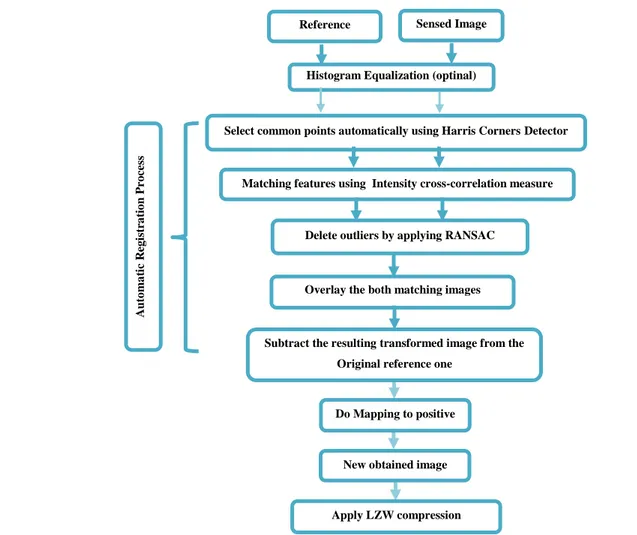
2- The Proposed Methodology:

(3)

Fig. 1: The Workflow for the Proposed Satellite Image Compression

2-1 Satellite Image Loading and Enhancement:

After loading the image file, the system passes the image through histogram equalization (HE) operation to enhance the image contrast and to facilitate features detection process. Histogram equalization is the most adopted contrast modification technique (Yeong-Taeg Kim, 1997), it stretches the dynamic range of the image histogram to obtain good contrast enhancement effect for images that look too dark or too bright. This step is essential for enabling correct feature detection and matching.

2-2 Image Registration:

To find the matching of two or more images taken at different times from different sensors or from different viewpoints, the image registration technique is used (Ardeshir Goshtasby, 2012). Here, the feature–based model was used to establish the corresponding two sets of features points; one from the reference and the other from sensed images (Rochdi Bouchiha, Kamel Besbes, 2013). This task include the use of Harris corner detector for extracting image features; which are named key points or GCPs (ground control points) for both reference image and sensed image. A comparison is made between the two sets of the features descriptors using correlation rules to get the similarities between these descriptors (Mohamed Tahoun et al., 2016). The corresponding pairs of GCPs will be used to perform the proper geometrical transformation to align the sensed image to be more fitted to the reference image (Medha V. et al., 2009).

2-2-1 Extracting Image Features:

This step involves detection of stable and invariant regions/points which represent the image local features. In the proposed method, Harris corner detector is used to detect corners, where corners are usually good features because of its locality and orientation invariance. This detector extends the principle of Moravec’s corner detector [Sch10]. This method uses a weighting window which makes the detector response insensitive to rotations effects, with each window, a score R is associated, shifting a window in any direction, determining

Apply LZW compression algorithm New obtained image

Subtract the resulting transformed image from the Original reference one

Do Mapping to positive Reference

Image

Sensed Image

Select common points automatically using Harris Corners Detector

Matching features using Intensity cross-correlation measure

Delete outliers by applying RANSAC

Overlay the both matching images

A

u

to

ma

ti

c

R

eg

ist

ra

ti

o

n

P

ro

ce

ss

(4)

which windows produce large significant change in all directions; i.e., mean it is a corner (Richard Szeliski, 2010); all windows that have a score R greater than a certain value are considered corners:

𝑀 = ∑ 𝑤(𝑥, 𝑦) (𝐼_𝐼𝑥𝐼𝑥 𝐼𝑥𝐼𝑦 𝑥𝐼𝑦 𝐼𝑦𝐼𝑦)

𝑥,𝑦 (1)

Where: W(x,y) is the weighting window over the area (x,y); (Ix, Iy) are the partial image derivatives in x and y directions, respectively.

The most common choice for the weighting window is Gaussian, because it makes the responses isotropic. A score R is calculated for each window (Harris, C., M. Stephens, 1988):

R =det (M) - k (trace M)2_{= λ}

1λ2 − κ (λ1 + λ2)2 (2)

Where, (λ1, λ2) are the Eigen values of the matrix; if both are greater than the given threshold (threshold=1000) it will be considered good feature (corner); K is a tunable parameter, it can be determined empirically, its value is set 0.04.

The implementation of Harris algorithm can be summarized as follows:

1. Compute the horizontal and vertical derivatives dx and dy for both images Ix and Iy. 2. Compute the three terms in the matrix M.

3. Apply Gaussian filter to convolve each of those images, this smoothing filter is important to ensure that the derivative is not picking up any noisy bits and the derivatives will be more delicate.

4. Compute R and determine if the detected good feature is a corner or not considering the given threshold.

2-2-2 Similarity Measures:

In this step the matching operation is performed by calculating the normalized cross correlation (NCC) (Mohamed Tahoun et al., 2016), which can be defined as:

NCC(A, B) =1

N∑

(A−μA)(B−μb)

σ_Aσ_B

x,y (3)

Where; N is the total number of pixels in image A and B; (μA, μB) are the mean of images A & B, respectively, for simplicity let the mean =0. While (σA, σB) are the standard deviation of images A and B, respectively.

The above equation can be used to directly compare the intensities in small patches around each feature point. After implementing (NCC) some of matching point pairs will wrongly correlated, for this reason the robust estimator RANSAC algorithm was used to remove the outliers; so the resulting contains only an enhanced list of correct matching points that demonstrates the actual matches list between the sensed and the reference images (Mohamed Tahoun et al., 2016). This algorithm performs very well to remove the outliers when there are no more than 50% outliers (Kai Zhang et al., 2014).

2-2-3 RANSAC (RANdom SAmple Consensus) algorithm:

RANSAC is an estimation method proposed by Fischler and Bolles, used for fitting the mathematical models (homographies) from sets of observed points after removing the outliers set from that observed points. In this method, for a number of iterations, a random sample of 4 correspondences (matches) is selected from the data set, and the homography H indicator is computed from that sample, then determining the outliers depending on its concurrence with H. After the last iteration is done, H (the desired mathematical model) is recomputed using the data set in the iteration that included the largest number of inliers (Mohamed Tahoun et al., 2016).

To use RANSAC, firstly a homography H is computed, it is an invertible projective transformation used in projective geometry to project the sensed image over the reference image to put the keypoints in the both images at the same scale and orientation. Homogeneous coordinates are very useful because it can directly perform matrix multiplication alone to implement the required projective transformation using 3x3 matrix with eight degree of freedom. The last value can determine as a scale parameter as following:

( 𝑥́ 𝑦́ 1

) = (

𝑎11 𝑎12 𝑎13 𝑎21 𝑎22 𝑎23 𝑎31 𝑎32 𝑎33

) ( 𝑥 𝑦 1

) (4)

Where: (x',y’,1) is the transformed coordinate of (x,y,1), the scale parameter =1 is for simplification. The minimum number of trials (N) used with the RANSAC algorithm to obtain success probability, is determined as follows:

N = log(1−p)

log(1−qs₎ (5)

Where: (p) is the probability of independent point pairs belonging to the largest group that can be mapped by the same transformation (Usually p = 0.99); (q) is the probability of finding the largest group that can be mapped by the same transformation; and (s) is the number of sample points.

RANSAC Algorithm Steps implies the following (Richard Hartley, Andrew Zisserman, 2003):

(5)

b.

While Si< T (the total number of random samples) Do: b1. Increment Si; Si ← Si+1;

b2. Randomly select a sample of 4 pairs of matching point and instantiate the model H from this subset using projective transform.

b3. Determine the set of data points that are within a distance threshold t (usually set to 0.95) of the model H to be inliers.

End Loop.

c.

After N trials the largest consensus subset Si is selected and used to re-estimate H.

2-2-4 Apply transformation function:

Images varying in resolution, rotation and view angle; so pixel locations in the reference image differs from pixel locations in the sensed one, to correct these geometric differences we need to perform geometric transformation functions; also called image rectification (Mohamed Tahoun et al., 2016). Here, the 1st_order affine geometrical transformation is applied; which performs linear mapping. It is a combination of linear transformation and translation. In 1st_{order affine transformations, the relation between two corresponding points} (x, y) and (X, Y) can be defined as:

x = m1+m2X+m3Y … (6a) y = n1+n2X+n3Y … (6b) Where: (m1, m2, m3) and (n1, n2, n3) are the transformation coefficients.

2-2-5 Evaluation of transformation operation:

To evaluate the transformation task, a suitable error metric must be chosen, the proposed method uses the similarity measurement (i.e., Mean Square Error: MSE) and it is computed twice. The first is between the reference and sensed image (MSE1), and second is between the reference and transformed image (MSE2). If the value of the error metric become smaller than the transformation is accepted. MSE is determined using the following formula:

MSE =1

N∑ ∑ (Img1(x, y) − Img2(x, y)) 2

, x

y (7)

Where, N is width x height.

2-3 Quantifies Difference Between Both Images:

In this step the resulting transformed image can be easily subtract from the reference one using the following criterion:

If (image1.size) not equal (image2.size) Return null;

Else

Diff = image2(x, y) - image1(x, y); Return Diff End if

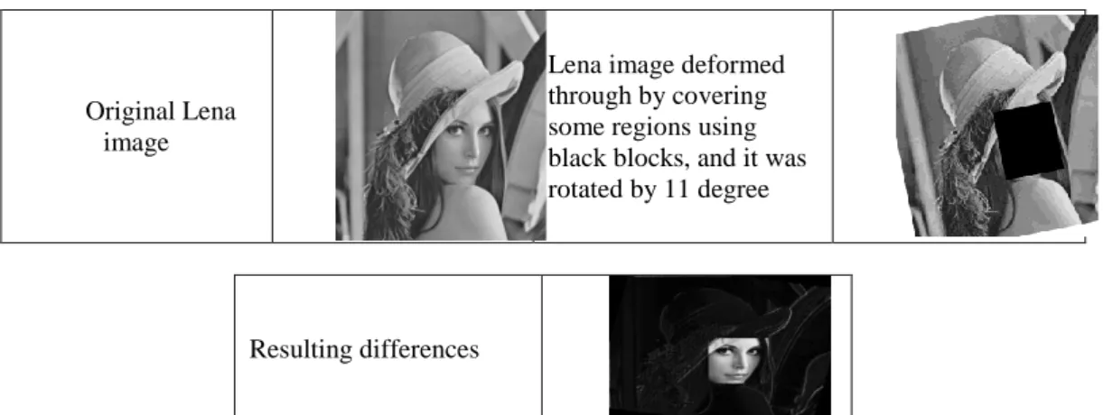
Original Lena image

Lena image deformed through by covering some regions using black blocks, and it was rotated by 11 degree

Resulting differences

Fig. 2: Lena original image and the distorted image with the resulting differences image

(6)

2-4 Mapping To Positive:

It means mapping pixels values to become always positive numbers; this can be satisfied through applying the following equation on each pixel (M) value (Shaymaa, D. Ahmed et al., 2015):

Mi= {

2Mi if Mi≥ 0 −2Mi+ 1 if Mi< 0 ,

(8)

2-5 Apply Shift Coding:

One of the major characteristics of the difference values is the small values (i.e., close to zero) are the most probable, but due to the little occurrence of some high values the use of fix length encoding for representing the difference image pixels values is not feasible. So, shift coding was applied to represent the pixels difference values, such that short codewords with little number of bits is used to represent the small valued pixels and long codewords are used to represent the large pixels values (Shaymaa, D. Ahmed et al., 2015).

2-6 Apply Lossless Compression:

As last stage, the proposed method used the common lossless compression algorithm, LZW (Lempel-Ziv-Welch) which is classified as a dictionary – based algorithm (Faisel Ghazi Mohammed, 2005). For images, the LZW encodes the strings of data which correspond to sequences of pixel values; it creates a table that includes the strings and their corresponding codes; this table is not stored with the compressed data. Coding a new string leads to insert the corresponding codes in the strings table. While the decompression operation involving extracting the strings table from the compressed data itself. In the introduced system, the compressor LZW is applied directly on the resulting differences image.

A comparison between the two compression results (i.e., applying LZW directly on the image, and the compressed data produced by the introduced system) is done using compression ratio (CR) as performance indicator.

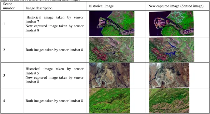
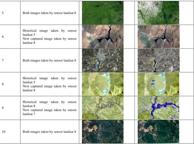
3- Test Image Data Sets:

To measure the performance of the proposed approach, a collection of remotely sensed land images are used as the test material which is chosen from “the Land Remote Sensing Image Gallery” in USGS web site [USG]. The chosen collection from this website “changes Over Time collection” provide a variety of remote sensing archive that record many different types of landscape changes through time for different areas from the worldwide. Table (1) show some of extracted scenes from that collection, left side contain the historical original image and the right side contain the newly captured image for the same scenes. The images in Tagged Image File format (TIFF), using sensors: landsat8, landsat7, landsat5, for more information see the source USGS.

Table 1: Subset of tested remote sensing land images Scene

number Image description Historical Image New captured image (Sensed image)

1

Historical image taken by sensor landsat 7

New captured image taken by sensor landsat 8

2 Both images taken by sensor landsat 8

3

(7)

6

8

9

4- Results:

The proposed compression scheme was implemented using C# programming language, working under the OS window 7 Ultimate. To evaluate the proposed method, the image data represented in table (1) was used; each original image was directly compressed using LZW. Then, the proposed compression scheme was used to compress the obtained differences image that came from subtracting the newly photographed image with different view angle (sensed image) from the original image for the same scene.

The statistical measure of randomness which called “Shannon Entropy” was used to characterize the 1st order statistical characteristics of both the sensed image and resulting difference one. Entropy is defined as (Shannon, C.E., 1948):

E=- ∑ P (i) log (P (i)) (9)

Where

P (i) = Histogram (i) ∕ no. of image pixels (10)

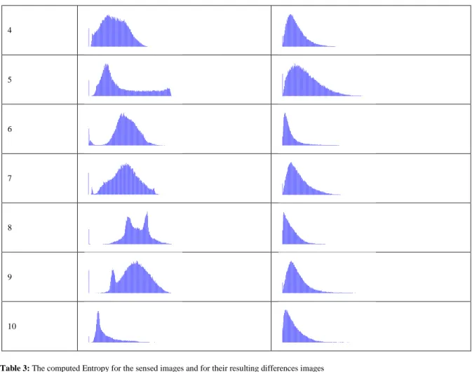
Table (2), (3) showed the comparisons of histogram and Entropy measures respectively between each case that listed in table (1) and the corresponding resulting difference image for each case. The results show that the histogram and Entropy values will always decrease for the resulting difference images.

Table 2: Histogram diagrams of listed image Data Sets and their resulting difference images

Scene number Histogram for sensed image Histogram of resulting difference image

1

2

(8)

4

5

6

7

8

9

10

Table 3: The computed Entropy for the sensed images and for their resulting differences images

Scene number for Sensed Image for Resulting Differences Image

Entropy measuring Standard deviation Entropy measuring Standard deviation

1 6.5990530 41.3071343 6.3755163 30.2016023

2 7.19697937 37.1028191 6.47117684 27.2805619

3 7.330340071 40.12972663 6.711703157 32.9203724

4 7.17175067 36.6571054 6.62208359 27.88653943

5 7.5508986 66.1586817 7.33157100 43.7695599

6 7.04651285 35.5671724 6.14147156 31.0050889

7 7.38714312 42.3533177 6.8097321 31.7510983

8 7.0328146 36.1128772 6.16138455 22.56381484

9 7.3462670 42.5006972 6.764500403 33.44818689

10 6.56228431 35.83087233 6.55208205 30.4638757

Also the compression ratio (CR) measure was computed for each case as shown in table (4). Firstly (CR) is computed for each case listed in table (1), denote by (CR1); then the (CR) is computed for the corresponding produced difference image which is denote by (CR2).

Table 4: calculate (CR1) for sensed images and (CR2) for their resulting differences images

Scene number CR(1) for compress whole sensed _image CR(2) for compress resulting difference image _only

1 1.03 4.2

2 1.02 3.72

3 1.01 3.75

4 1.04 3.64

5 1.73 3.42

6 1.01 3.98

7 1.01 3.61

8 1.00 3.94

9 1.02 3.58

10 1.00 3.78

(9)

performance is the same for other scenes in the dataset, and due to space constraints, these results are not presented.

5- Conclusion and Future Work:

In this paper, a fast lossless developed compressor for sequences of satellite images based on inter-frame coding and LZW method has been proposed. As shown, the introduced compression method is based on removing the temporal redundancy that exists between the satellite images taken for specific region under different conditions. The method uses image registration process to align the new sensed image with existing reference image. The registration process was done to minimize the difference between both images as much as possible. Also, the method involves extracting the two required sets of the keypoints using Harris corner detector and their descriptors using normalized cross correlation measure, using robust estimation RANSAC method to remove outlier points and generate the best mapping affine transform required to be applied on the sensed image to overlay it with the reference one.

Then, the applied next step is subtracting the two images (reference image & new mapped image), doing this will reduce the size of data that needed to be compressed. The next stage was applying mapping to positive to remove the negative values from the obtained difference numbers. Then, the outcome positive difference values are coded using shift-key coding method. Finally, the LZW compression method was used as the lossless compression method.

The results of conducted tests show that high (CR) can be attained when using the proposed compression scheme, it is better than the attained (CR) when LZW compression is applied on the whole new satellite image.

For future work the following topics need to be further discussed:

 Further sensor images are recommended to reach more decisive conclusions about the performance of the introduced method.

 Design a lossy compression algorithm as a substitute for lossless compression algorithm.

 Design a system for organizing dataset for the used references satellite images.

REFERENCES

Ardeshir Goshtasby, 2012. “Image Registration Principles, Tools and Methods”. ISSN 2191-6586 e-ISSN 2191-6594, Advances in Computer Vision and Pattern Recognition ISBN 4471-2457-3 e-ISBN 978-1-4471-2458-0 DOI 10.1007/978-1-978-1-4471-2458-0 Springer London Dordrecht Heidelberg New York, pages(1-5).

Delaunay, X., M. Chabert, V. Charvillat, G. Morin, 2009.” Satellite image compression by post- transforms in the wavelet domain”. Elsevier B. V.

Faisel Ghazi Mohammed, 2005.” Color image Compression Based DWT”. A thesis Submitted to the Collage of Science University of Baghdad In Partial Fulfillment of the Requirement for the Degree of Doctor of Philosophy in Astronomy Science.

Harris, C., M. Stephens, 1988: “A combined corner and edge detector”. In: Proceedings of the 4th Alvey Vision Conference (AVC), pp: 147-151.

Jagadeesh Kumar, Dr.P.S., 2015. “A comparative case study on compression algorithm for remote sensing images”. Final manuscript for publication in WCECS, SanFrancisco, USA, October, ICSPIE’

Jager, F., 2011. “Contour-based segmentation and coding for depth map compression”. In Proceedings of IEEE Visual Communications and Image Processing, pp: 1-4.

Kai Zhang, XuZhi Li, JiuXing Zhang, 2014. “A Robust Point-Matching Algorithm for Remote Sensing Image Registration”. IEEE geosciences and remote sensing letters, 11: 2.

LIU XiJia, TAO XiaoMing, GE Ning, 2015.” Remote sensing image compression using priori information and feature registration”,978-1-4799-8091-8/15/$31.00, IEEE

Medha V. Wyawahare, Dr. Pradeep M. Patil, and K. Hemant, 2009. Abhyankar. “Image Registration Techniques: An overview”. International Journal of Signal Processing, Image Processing and Pattern Recognition 2: 3

Minqi Li, Quan Zhou, and Jun Wang, 2008. “Remote Sensing Image Compression Based on Classification and Detection”. PIERS Proceedings, Hangzhou, China

Mohamed Tahoun, Abd El Rahman Shabayek, Hamed Nassar, 2016. “Satellite image matching and registration: A comparative study using invariant local features”. © Springer International Publishing Switzerland. A.I. Awad and M. Hassaballah (eds.), “Image Feature Detectors and Descriptors”, Studies in Computational Intelligence 630, DOI 10.1007/978-3-319-28854-3_6

Muthukumaran, N., R. Ravi, 2014.” The performances analysis of fast efficient lossless satellite image compression and decompression for wavelet based algorithm”. Springer Science + Business Media New York

(10)

Richard Hartley, Andrew Zisserman, 2003. “Multiple view geometry in computer vision”. Cambridge University Press, second edition.

Richard Szeliski, 2010.” Computer Vision: Algorithms and Applications”. September 3, 2010 draft c, Springer.

Rochdi Bouchiha, Kamel Besbes, 2013.” Comparison of local descriptors for automatic remote sensing image registration”. DOI 10.1007/s11760-013-0460-3. © Springer-Verlag London.

Schmidt, A., M. Kraft, A.J. Kasinski, 2010: “An evaluation of image feature detectors and descriptors for robot navigation”. In: ICCVG (2)’10: 251-259.

Shannon, C.E., 1948. “A Mathematical Theory of Communication”. Reprinted with corrections from The Bell System Technical Journal, 27: 379-423, 623–656.

Shaymaa, D. Ahmed et al., 2015. “The use of cubic Bezier interpolation, biorthogonal wavelet and

quadtree coding to compress color images”, British journal of applied science & technology.

Shichao Zhou, Chenwei Deng, Baojun Zhao, 2015.” Remote sensing image compression: R review”. IEEE International Conference on Multimedia Big Data.

https://remotesensing.usgs.gov/gallery/index.php, USGS website, date stamp: 12/2/2017.