Document downloaded from. The final publication is available at: Copyright.

Document downloaded from http://hdl.handle.net/10459.1/47764

The final publication is available at: https://doi.org/10.1002/asmb.2034

Copyright

(c) John Wiley & Sons, 2014

The persistence of abnormal return on assets: an exploratory

analysis of the performance of firms by country and sector

José Luis GALLIZO e-mail: [email protected] Department of Business Administration and Economic Management of Natural Resources UNIVERSITY OF LLEIDA Pilar GARGALLO e-mail: [email protected]

Department of Economic Structure and History and Public Economics UNIVERSITY OF ZARAGOZA Ramon SALADRIGUES e-mail: [email protected] Department of Business Administration and Economic Management of Natural Resources UNIVERSITY OF LLEIDA Manuel SALVADOR e-mail: [email protected] Department of Economic Structure and History and Public Economics UNIVERSITY OF ZARAGOZA

Abstract

This study offers an exploratory statistical analysis of the persistence of annual abnormal returns across a sample of firms from different European Union (EU) countries. To this end, a hierarchical Bayesian dynamic model has been used which enables the annual behaviour of those profits to be broken down into a permanent structural component and a transitory component, while also distinguishing between general effects affecting the industry as a whole and specific effects impacting on each firm in particular. This breakdown of the behaviour of profits allows for a more accurate assessment of the relative importance of these fundamental components by country and sector. Furthermore, through the Bayesian approach it is possible to test different hypotheses about the homogeneity of the dynamic behaviour of the above components with respect to the sector and the country where the firm develops its activity.

We find that, although both the industry and firms effects are significant, the latter are more important to explain the dynamic evolution of abnormal returns. Specifically, firm effects account for 68% of total variation of the abnormal returns and display a lower degree of persistence with adjustment speeds oscillating at around 34%, while industry effects only account for 9% and have adjustment speeds oscillating between 7%-8%. However, this pattern is not homogeneous, and depends on the sector and country in which the firm carries out its activity. These results highlight the need to take into account both aspects simultaneously in order to analyse the dynamic behaviour of abnormal returns.

Keywords: Dynamic models, Bayesian Inference, MCMC, Abnormal Returns, Persistence of Profits, Return on Assets

1. INTRODUCTION

According to Economic Theory, the profit rates of firms in competitive markets should converge towards the mean of the market, although this is not always the case. Some empirical studies have found differences between firms that persist over time (Jacobson, 1988) varying the speed with which they adjust their benefits to stable values (Geroski and Jacquemin 1988; Waring, 1996; Glen et al., 2003). Other studies have described the evolution over time of such profits with the aim of analyzing whether the differences are transitory, and tend to disappear with the passing of time, or permanent, tending to persist over time (see, for example, Waring, 1996; McGahan and Porter, 2003).

Bou and Satorra (2007) have proposed a dynamic model which allows firms’ abnormal returns to be decomposed into a permanent, a transitory and a specific component. Their method is particularly interesting because it enables evaluation of the importance of each component as well as the distinction between shocks which affect the firm sector as a whole and specific shocks which affect each firm. These authors studied the behaviour of 5,000 Spanish firms over the period 1995-2000 and concluded that significant permanent differences exist at both, sector and firm levels, the latter differences being of greater magnitude. However, they did not observe significant differences among the adjustment processes of the transitory components which operate at both sector and firm levels.

Gallizo et al. (2007) extended this study to different European countries using a larger sample of firms. They observed a low persistence of the transitory component due to the growing degree of competitiveness in the business context of the countries studied. This behaviour is not homogeneous but depends on the sector and country. However, the authors do not distinguish between shocks with an impact on the industry as a whole and those affecting individual firms.

The present study consists of an extension of Gallizo et al. (2007) and is, to the best of our knowledge, one the first studies that considers industry and firm effects and evaluates the importance of both types of effects. The research has an exploratory character and analyses the persistence of annual profits across a sample of firms from different European Union (EU) countries while taking into account the sector and the country where the firm develops its activity. To this end, we adopt the framework proposed by Bou and Satorra (2007) to analyse a large sample from different EU countries.

The results of the analysis are consistent with previous studies in showing that although the impact of industry-wide shocks is significant, the specific shocks upon each firm are still more important. Furthermore, our study proves that the industry effect, the importance of the different components (permanent, transitory, idiosyncratic) and the short and long-term behaviour of the profits depend on the sector and country in which each firm carries out its activities. All of the above suggest the need for taking into consideration these two aspects in order to analyse the dynamic behaviour of the abnormal profit rates. Thus, the innovative character of the present study can be summarised into the three following aspects:

a) An analysis of the homogeneity of industry and firm effects by country and sector considering all the available information simultaneously.

b) The application of a Bayesian methodology that allows precise inferences about the parameters of the considered models without using asymptotic results, which in this context (small T and N in some country-sector combinations) could have dubious validity.

c) A model comparison process performed by considering the goodness of fit and the parsimony of the compared models (some of which are non-nested) at firm and sector-country levels. In this way, a most comprehensive study on the persistence of benefits is carried out from different perspectives.

The study is organised as follows: section 2 explains the data used, section 3 describes the model and statistical methodology adopted, section 4 presents the results obtained, and section 5 draws some conclusions. In addition, the paper contains one appendix with the statistical procedures used to estimate and compare the different models considered in the paper.

2. DATA

The source of the data analysed is a sample of 23,293 firms in 6 EU countries selected from the AMADEUS database (2009 version), which was developed by Bureau van Dijk with comparable financial information for private firms across Europe. The choice of the database was due to its coverage and the quality of the data available for each firm. In terms of coverage, the study requires firm-level data to be available across time and across sectors at a relative level of disaggregation (NACE Rev. 2- 3 digits). Since our analysis

focuses on comparability across members of the EU, we prioritise the data derived from a common international source, rather than a set of national ones, in order to avoid possible different criteria.

The period analysed covers from 1999 to 2007 and the frequency of observation is annual. A total of 21 sectors were considered, and the selection was made in order to include a large number of firms in each country-sector combination. This would allow us to estimate industry effects accurately enough so that meaningful comparisons could be made by sector and country. The first 8 (NACE code < 400) belong to the manufacturing sector, the last 12 to the services sector while sector 432 belongs to the construction sector.

The goal in data collection was to ensure we had a sufficient number of firms for each country/industry combination rather than develop a global study for firms in the EU. For this reason, we decided not to include the industries ex-ante. We selected firms with at least 6 years of return on assets (ROA) in the period and industries with at least 30 firms for each country/industry combination. Firms correspond to 21 sectors and 6 countries, and the number of total observations was 208,112. The profit ratio analysed is the ROA and the percentage of firms with missing data was equal to 6.5%, all of them corresponding to 1999. Table 1 shows the composition of the sample by countries and sectors. The most represented countries are France, Spain, the United Kingdom and Italy, which reflects their larger specific weight within the EU. There is no particular preponderance of any sector, thus permitting comparisons to be made at sector level.

(Insert Table 1 around here)

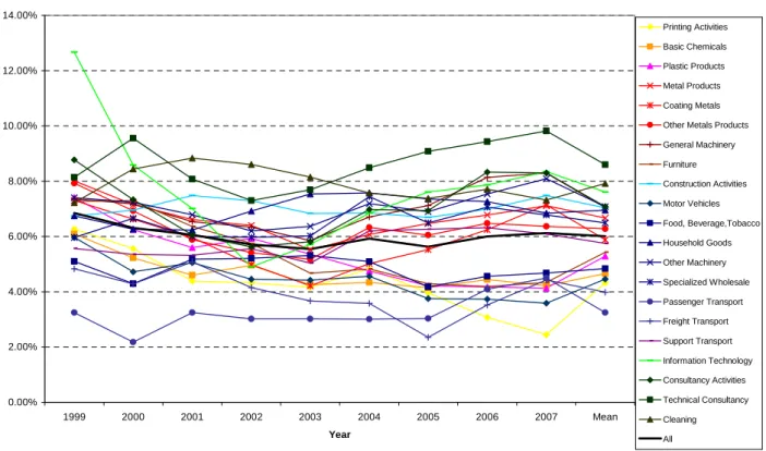
Figures 1 and 2 show the annual evolution of the average ROA value by country and by sector, respectively. Average ROA for all the firms in the sample was around 6%, it decreased in the period 1999-2002 and increased thereafter. By country, the highest values for ROA were achieved by Swedish firms, whose ROA was around 8.30%, but with more marked decreasing (period 2000-2003) and increasing (period 2004-2007) trends. The smoothest evolution corresponded to the Italian and Spanish firms whose average ROA had a decreasing trend throughout the period. From Figure 2 it can be seen that for most sectors the average ROA remained more or less constant throughout the period. However the annual standard deviations of ROA were high, oscillating around 11% in countries and 6% in

sectors, which highlight the existence of high levels of heterogeneity in the dynamic evolution of ROA firms along the analysed period1.

(Insert Figures 1 and 2 around here) 3. STATISTICAL METHODOLOGY

This section offers a brief description of the statistical methodology employed in the study. Mathematical details can be found in the Appendix.

3.1. Set-up

Data correspond to ROA (hereinafter R) of a sample of N firms, measured over the period {1,…, T}.

Let {Rit; tTi {1,…, T}; i=1,…, N} where Ti = {tlow,i, tlow,i+1, …, tupp,i} with 1≤tlow,i<tupp,i ≤ T denote the periods of time for which information is available for iith firm. Let yit = Rit – Rmean, t be the value of abnormal return for ith firm in the period t, where

Rmean,t =

t t t t :i

t , i N

R i , upp i , low



 

is the mean of ratio R in the period t and Nt = cardinal{i{1,…,N}: tlow,i ≤ t≤ tupp,i} is the number of firms with observed ROA for the period t.

Let s(i)S={1,…, S} be the sector in which ith firm develops its activity, where S is the number of sectors considered in the study.

Let c(i)S={1,…, C} be the country in which ith firm develops its activity, where C is the number of countries considered in the study.

3.2. The model

We adopt the framework of Bou and Satorra (2007) and we split up the abnormal profitability of a firm into 3 components: an industrial component, YI, which reflects the influence of permanent and transitory effects impacting on the industry to which the firm belongs; a firm-specific component, YF, which reflects the influence of specific permanent and transitory effects that affect each firm individually; and, finally, an idiosyncratic component, U, which reflects the influence of specific and occasional shocks which do no persist over time.

However, in order to analyse the homogeneity of the above components, we introduce three classification functions G, L: {1, …, N} {1,…, C}x{1,…, S}, and H:

Im(G)=G({1,…,N}) {1,…, C}x{1,…, S}, where G indexes firms with the same industry component, L indexes firms whose firm component evolves in a similar way, and H indexes industry components evolving in a similar way.

The model’s equations are given by:

yi,t = yI,G(i),t + yF,i,t + ui,t = pI,G(i) + aI,G(i),t + pF,i + aF,i,t + ui,t with ui,t ~ N



0,u2,L i,t



; tTi (3.1)

pI,G(i) ~ N



0,p2I,HG(i)



(3.2)

aI,G(i),t+1 = I,HG(i)aI,G(i),t + dI,G(i),twith dI,G(i),t ~ N



0,2aI,HG i



; t *

) i ( G

T -



*



) i ( G , low

t (3.3)

   

   

  

  

2 ) i ( G H , I 2

) i ( G H , a t

), i ( G ,

I ~N 0,₁

a I

* ) i ( G , low

(3.4)

pF,i ~ N



0,2pF,L(i)



(3.5)

aF,i,t+1 = F,L(i) aF,i,t + dF,i,t with dF,i,t ~ N



0,2aF,L(i)



; tTi-{tlow,i} (3.6)

    

  

  

2 ) i ( L , F 2

) i ( L , a t

, i, F

1 , 0 N ~

a F

i , low

(3.7)

ui,t ~ N



0,_u2_,t



; tTi (3.8)

where



*



g , upp *

g , low *

g t ,...,t

T  with _{i G   g }

 

lowi, *

g ,

low min t

t  _ 1 , _{iG   g} 

 

uppi, *

g ,

upp max t

t  _ 1 is the

observed period corresponding to group gIm(G), {ui,t; tTi ; for i=1,…, N} are independent errors and

yI,G(i),t is the value of the industry component of firm i yF,i,t is the value of the specific component of firm i

pI,H(G(i)) is the permanent component of yI,,G(i),t . This component captures the difference existing between the groups of firms indexed by G, due to their structural features or the nature of their activity, differences which tend to persist in the long term.

aI,H(G(i)),t is the transitory component of yI,,G(i),t. It represents the temporary differences existing in period t between the groups of firms indexed by G, which tend to disappear with time and where the parameter -1<I,H_G(i)_<1 quantifies the component’s persistence over time.

pF,I is the permanent component of yF,i,t . It reflects the differences existing among firms which are due to their specific structural features, features which tend to persist in the long term.

aF,i,t is the transitory component of yF,i,t . It captures the firm’s specific temporary differences in the period t, which tend to disappear with time, where -1<F,L(i)<1 quantifies the component’s persistence over time.

ui,t is the idiosyncratic component for each firm in the period t. It indicates the influence exercised by occasional events specific to each firm which occurred in period t but whose effect has not any persistence over time.

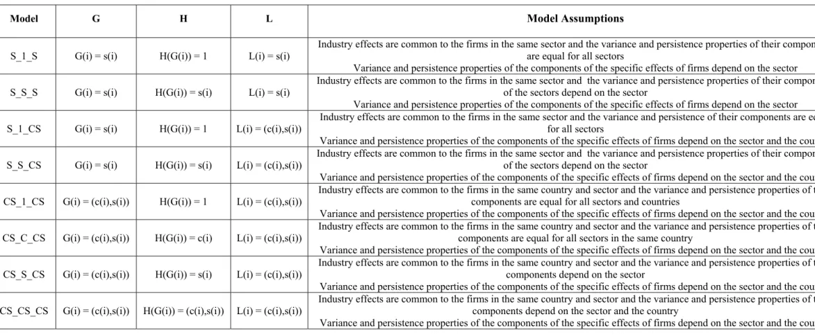
It is worth pointing out that, unlike Bou and Satorra (2007), we do not assume that the variance and persistence of the permanent and transitory components are common to all the firms. This evolution is determined by G, L and H functions which index groups with similar behaviour with respect to these components. Some assumptions and the corresponding G, L and H functions are given in Table 2. Other possible assumptions were also considered, but their results were worse than those discussed in the paper and they are omitted for the sake of brevity.

(Insert Table 2 about there) 3.3. Estimation and comparison of models

The model parameters were estimated following a Bayesian approach described in the section A.1 in the Appendix. This approach allows us to make exact inferences which reflect the uncertainty associated with the estimation process. In addition, Bayesian methodology allows us to carry out non-nested and nested model comparison processes using criteria that quantify their predictive behaviour and their goodness of fit to data (see section A.2 in the Appendix, expressions (A.8) to (A.18)). Using these tools we can choose the most adequate model specification and analyze the significance of its components. 4. RESULTS

4.1. Comparison and simplification of models

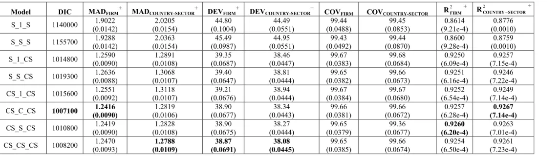
Table 3 shows the results of the comparison of models listed on Table 2. It can be seen that best models (CS_C_CS, CS_S_CS and CS_CS_CS) assume that the variance and persistence of the specific firm effects depend on the firm’s country and sector.

However, things are not so clear with respect to the industry effects. Models which assume that industry effects properties are common to firms in the same country and/or sector have the best performances, but the homogeneity in variance and persistence of these effects are not clearly determined. CS_C_CS model is the best with respect to DIC, MADFIRM and R2COUNTRYSECTORcriteria; R2FIRMcriterion selects CS_S_CS as the best model

and, finally, CS_CS_CS model is the best with respect to MADCOUNTRY-SECTOR and DEV criteria. This reflects the similarity of the estimated values of the persistence coefficients I for most countries and sectors (Tables 5a and 5b).

All these models have an adequate goodness of fit to data, with 2 FIRM

R and

2

SECTOR COUNTRY

R _ higher than 0.9250, and adequate coverage properties of the 99% Bayesian credibility intervals (see Table 3).

We need to point out that this lack of statistical evidence to discriminate whether sector, country or both aspects should be taken into account in order to explain the evolution of industry effects may be due to the low number of observations by series and the low number of sectors and countries considered in the study. This fact raises the uncertainty level of the estimation of the variance and persistence parameters of the industry effects causing their non-significance. In order to increase the precision level of the estimations, future research should expand the number of time periods and the number of firms.

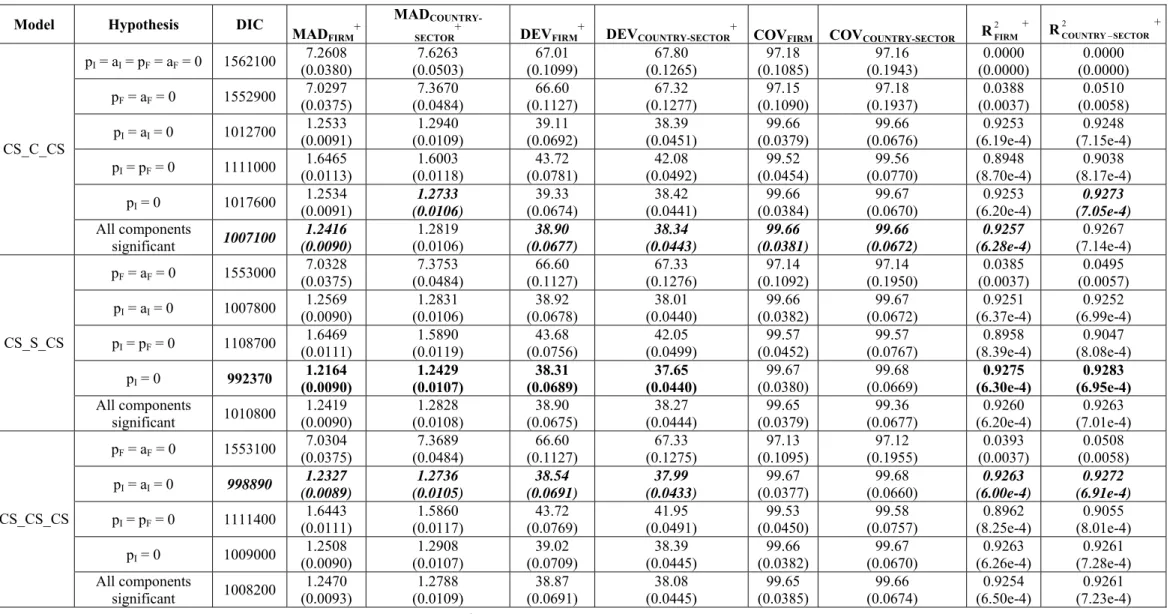
Table 4 shows the results of the simplification process of the best performance models where we analyse the joint statistical significance of the components of the industry and firm effects. With this aim, we consider the following assumptions:

Hnone: pI,i = aI,i,t = pF,i = aF,i,t = 0; tTi; i=1,…, N (all components are non-significant ) Hindustry: pF,i = aF,i,t = 0; tTi; i=1,…, N (only industry effects are significant)

Hfirm: pI,i = aI,i,t = 0; tTi; i=1,…, N (only firms effects are significant) Htransitory: pI,i = pF,i = 0; tTi; i=1,…, N (only transitory components are significant) Hno permanent industry: pI,i = 0; i=1,…,N (permanent component of industry effects are non

significant)

Hindustry-firm: All components of model (3.1) significant (Insert Table 4 about here)

Components of the specific firm effects are significant in all the models (pF≠0, aF≠0). Industry transitory component (aI) is significant in models CS_C_CS and CS_S_CS, while the industry permanent component (pI) is non-significant in all the models. Model CS_S_CS with constraint pI = 0 has the best performance with respect to all of the comparison criteria. 4.2. Estimation of parameters

In this section we show the results corresponding to the estimation of the parameters of the models. These results are shown by country and sector.

4.2.1. Persistence coefficients

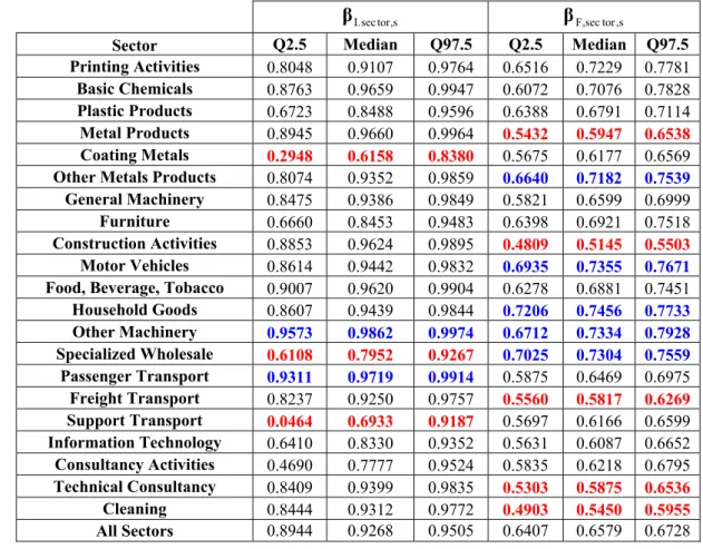
Tables 5a and 5b show the estimations of the persistence coefficients of the transitory components of the industry and specific firm effects, I and F, for firms grouped by country and by sector, respectively. Specifically, we provide the posterior median and the limits of the 95% Bayesian credibility intervals of each parameter built from the 2.5% (Q2.5) and 97.5% (Q97.5) posterior quantiles. Besides, we analyse the homogeneity of I and F by country and sector, by comparing their values with their median (denoted as I,country,all and

I,sector,all for I and as F,country,all and F,sector,all for F) for all the firms.

From Table 5a it can be seen that median industry persistence coefficient for all countries is 0.8924. Therefore, the global industry effect has a high persistence, with adjustment speed to shocks affecting the whole industry (1-I) equal to 10.76%. This result is consistent with the smooth annual evolution of the average ROA (see Figure 1). On the contrary, the specific effects are significantly less persistent, with a median persistence coefficient, F,country,all, equal to 0.6596 with an adjustment speed equal to 34.04%.

(Insert Table 5a and 5b about here)

Nevertheless, the homogeneity hypothesis by countries is rejected: the persistence of Italian and, to a lesser extent, Spanish industries is higher (0.9534 and 0.9313, respectively), while the persistence of Swedish industries is significantly lower (0.7334). These results are consistent with the annual evolution of their average ROA shown in Figure 1 where, as commented in section 2, higher oscillations of average ROA for Swedish firms can be due to its sharp decreasing (period 2000-2003) and increasing (2004-2007) trends. Statistically significant differences are also appreciated with respect to the specific adjustment coefficient F. The lower median persistence coefficients correspond to UK firms (0.5501) while Italian (0.7143) and Spanish (0.6907) firms show higher persistence levels.

We believe that there are not many published studies that analyse the persistence of European firms. A few papers (Yves and Weber, 1990, for France, or McMillan and Wohar, 2011, for the UK) assume that each firm has its own persistence coefficient, but they do not distinguish between industry and firm effects and, therefore, their results are not comparable to ours. Only in the case of Spain, Bou and Satorra (2007) did a similar study and found that persistence coefficients, for both industry and firm effects, were 0.64, which is a different result from our estimations (0.9313 and 0.6907, respectively). The discrepancy corresponds to the estimation of the persistence of the industry effects and it is due to the fact that we have estimated them using three-digit SIC codes, while those authors used four-digit SIC codes. The industry effects calculated using three-digit SIC codes correspond to average behaviours of ROA of bigger groups of firms than those calculated using four-digit SIC codes groups. Therefore, their evolution is smoother and their persistence is higher.

Table 5b shows that the median industry persistence coefficient for all sectors is 0.9268 (adjustment speed equal to 7.32%) while the median specific firm coefficient is 0.6579 (adjustment speed equal to 34.21%). These values are similar to those shown in Table 5a which confirms the robustness of the previous results. The homogeneity hypotheses of I and F coefficients are also rejected by sectors because there are sectors whose coefficients are significantly different from their median values.

An analysis of F2was also made by country and sector combinations. However, it has not been included in this paper for the sake of brevity3. The results of this analysis highlight that there is greater rigidity in southern countries and more flexible markets in Northern European countries. While the majority of sectors with greater persistence is located in Italy and Spain, the sectors with lower persistence are located in the United Kingdom and Sweden. These results are consistent with statistical studies on employment, according to which Italy and Spain were, in the period analysed in this paper (1999-2007), two of the countries with a more rigid labour market and higher costs in unfair dismissals, compared to the UK which had greater labour flexibility (Pin et al, 2007).

2 _{Remember that, according to Table 3, model CS_CS_CS rejects the significance of industry effects and, for} this reason, this study was not made for I

4.2.2. Permanent component of the firms

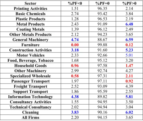
In this section we analyse the specific permanent component (pF) of the firms. This component coincides with the firm permanent component (pI+pF) given that, according to results of Table 3, pI is non significant. We show for each country (Table 6a) and sector (Table 6b) the percentage of firms whose permanent component is significantly negative (PF<0), non-significant (PF=0) and positive (PF>0). This statistical significance was determined by means of their 95% Bayesian credibility intervals, analysing whether these intervals contained or did not contain the value 0. It can be seen that most firms (94.15%) do not have a significant component, as is predicted by Economic Theory, with only 2.20% and 3.65% of firms having a systematic trend having lower and higher profits than the market.

(Insert Tables 6a and 6b about here)

There are no noticeable differences among countries. Belgium has the higher percentage of firms with non-significant permanent components (97.90%) while France, Italy and Spain have a slightly higher percentage of firms (around 4.10%) systematically outperform the market. By sectors, the behaviour is not so homogeneous. There are sectors (Furniture, Household Goods, Specialized Whole Sale or Passenger Transport) with a high percentage of firms whose permanent component is non-significant (greater than 97%). In other sectors (General Machinery, Information Technology, Cleaning, Metal Products and Construction of Activities) this percentage is significantly lower (less than 92%). Furthermore, in these sectors the percentage of firms which systematically out-perform the market (PF>0) is higher than those which systematically under-perform it (PF<0).

An additional study carried out by country and sector combinations revealed that for an important percentage of these combinations (38.89%) the existence of firms with significant permanent components was not appreciated. However, there are combinations (most of them located in the southern countries) with noticeable percentages of firms which systematically out-perform (PF>0) or under-perform (PF<0) the market4.

4.2.3. Importance of the components

Next, we will discuss the importance of industry and specific effects as well as the permanent, transitory and idiosyncratic components of model (3.1)-(3.8). With this goal, we

4 _{See Appendix B of Gallizo et al. (2013)}

estimate the percentage of the variance of the abnormal return of a firm which is explained by each component. We start from the variance decomposition

var(yi,t) = var



p_I,G(i)



var



a_I,G(i),t



var

 

p_Fi, var

 

a_Fi,,t var

 

u_i,t =

= 2

t ), i ( L , u 2 ) i ( L , F 2 a 2 p 2 )) i ( G ( H , I 2 a 2 )) i ( G ( H , p 1 1 ) i ( L , F ) i ( L , F )) i ( G ( H , I

I  

        

which follows from (3.1). The percentage of variation total in the ith firm explained by a given component is given by the generic expression:



               T 1 t 2 t ), i ( L , u 2 ) i ( L , F 2 a 2 p 2 )) i ( G ( H , I 2 a 2 )) i ( G ( H , p 2 i, component T 1 1 1 100 ) i ( L , F ) i ( L , F )) i ( G ( H , I I (4.1) where                             



 u component if T 1 a component if 1 p component if a component if 1 p component if T 1 t 2 t ), i ( L , u F 2 ) i ( L , F 2 a F 2 p I 2 )) i ( G ( H , I 2 a I 2 )) i ( G ( H , p 2 i, component ) i ( L , F ) i ( L , F )) i ( G ( H , I I (4.2)

Using (4.1) we calculate the average percentage for all the firms, for each country, for each sector, and for each country and sector. They are particular cases of the generic expression:





                Group i T 1 t 2 t ), i ( L , u 2 ) i ( L , F 2 a 2 p 2 )) i ( G ( H , I 2 a 2 )) i ( G ( H , p 2 i, component Group T 1 1 1 100 N 1 ) i ( L , F ) i ( L , F )) i ( G ( H , I I (4.3)

where NGroup is the number of firms included in the corresponding Group. We analyse the importance of the industry and the specific firm effects by adding the corresponding permanent and transitory percentages. Additionally, we analyse the importance of the permanent, transitory and idiosyncratic components, by adding the corresponding industry and specific firm percentages.

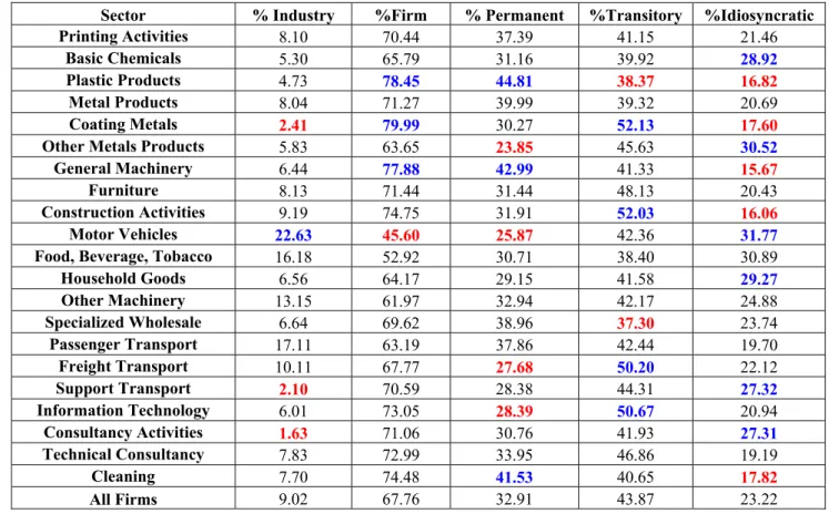
Tables 7a and 7b show the posterior means of the averages percentages for each country and sector, respectively. It can be seen (Table 7a row All firms) that most of the

total variation (67.76%) is explained by firm specific effects, while industry effects have a very marginal impact (9.02%)5. Also, the transitory effects are preponderant (43.87% of total variation) over permanent (32.91%) and idiosyncratic (23.22%) effects; this last result underlines the greater importance of temporary shocks for the evolution of firm abnormal returns.

An analysis of the importance of each effect for each country (Table 7a) shows that this pattern is not homogeneous. Specific firm effects have greater impact in French firms (74.04%), industry effects in Italian ones (12.36%) and idiosyncratic effects in Swedish (28.56%) and UK firms (28.57%). By components, it can be seen that in southern countries (Italy, France and Spain) the permanent component is more important (more than 35% of total variation) than in northern countries (Sweden, United Kingdom) where the transitory component is more influential by explaining more than 47%.

The greater persistence of Italian and Spanish firms (Table 5a) points to the high importance of their permanent component and highlights the greater rigidity of their markets with a trend of their firms to maintain their relative positions throughout the period analysed. It is a generally accepted fact that the rigidity in labour markets is one of the causes of the high unemployment rates of the Spanish economy. The same argument can also been applied in the Italian case (OECD, 2013). In contrast, the United Kingdom and, to a lesser extent, Sweden, have more dynamic markets with lower persistence levels and more important transitory and idiosyncratic components. It is also well known that in Sweden, the maintenance of its fiscal framework, the promotion of the highest occupancy of the workforce with flexible legislation, and the increase in the efficiency of public spending between 2000 and 2007 allowed the country to face negative shocks in more favourable conditions than in other European countries (OECD, 2011). Also, in this period, the lower rigidity of the economy in the UK allowed it to achieve a per capita GDP growth higher than any of the G6 countries (Corry et al., 2011). All this indicates a greater ability of firms in these two countries to adapt to external shocks materializing in better outcomes for their economies.

5 _{These values are not significantly different from those estimated by Bou an Sartorra (2007) in the case of} Spain.

(Insert Table 7a about here)

If we repeat this analysis by sectors (Table 7b) the existence of different patterns can be appreciated. With respect to industry and specific firm effects, there are sectors such as, Sale of Motor Vehicles, where the industry effects have significant importance by explaining 22.63% of the total variation. In contrast, there are some sectors such as Support Transport, Consultancy Activities or Coating Metals where these industry effects are clearly less important (less than 2.5% of total variation). There are also other sectors (Coating Metals, Plastic Products and General Machinery) where the specific firm effect has a significant higher degree of relevance and explains a greater percentage of total variation.

If we analyse the components of the model, we find sectors (Plastic Products, General Machinery and Cleaning) with an important permanent component (more than 41% of total variation), while in other sectors (Other Metal Products, Motor Vehicles, Freight Transport and Information Technology) these components are significantly less important (less than 29% of total variation). Additionally, there are some sectors (Coating Metals, Construction Activities, Freight Transport and Information Technology) where transitory components have significantly greater importance (more than 50% of total variation) while, in contrast, in Specialized Wholesale or Plastic Products, the importance of this component is significantly lower (less than 40% of total variation).

(Insert Table 7b about here)

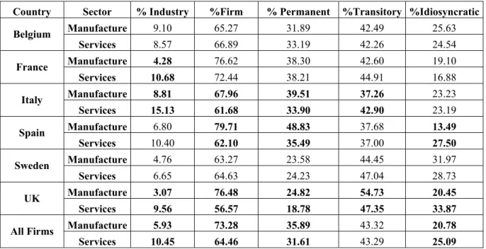
In order to analyse the existence of more generic differences, we show in Table 8 the average percentages of total variation explained by industry and firm effects and by the permanent, transitory and idiosyncratic components of the model corresponding to manufacturing ((NACER codes lower than 400, see Table 1) and services-based firms (NACER codes greater than 450) in the sample.

It can be seen that manufacturing firms have more important specific effects (73.28% versus 64.46% of total variation) and less important industry effects (5.93% versus 10.45% of total variation) than services-based firms. Exceptions to this rule are Belgium and Sweden, where significant differences between both types of firms are not appreciated. Furthermore, permanent components are more important in manufacturing firms (35.89% of total variation) than in services-based firms (31.61% of total variation), with this difference being significantly stronger in Spain and the United Kingdom and, to a lesser extent, in Italy. In contrast, the idiosyncratic effects component is more important in services-based

firms (25.09% of total variation) than in manufacturing firms (20.78% of total variation) with these differences being particularly stronger in Spanish and British firms.

All of these differences are mainly due to the lower capital intensity of services-based firms, which allow for a better adaptation to changes. Furthermore, in Spain, Italy and the United Kingdom, services-based firms are usually related to the very competitive sector of tourist activities, which explains the lower importance of permanent components.

(Insert Table 8 about here)

Finally, the analysis carried out by country and sector combinations revealed the existence of a great number of country-sector groups with significant differences with respect to the relative importance of the industry and firm effects. This result highlights the need to take into account both aspects of the firm in order to analyse the dynamic evolution of its abnormal returns6.

5. CONCLUSIONS

This study carries out a Bayesian statistical analysis of the dynamic evolution of abnormal returns in a sample of EU firms, taking into account the country and the sector where the firm develops its activities. To that end, a hierarchical Bayesian model based on Bou and Satorra (2007), has been used. The model allows us, on the one hand, to decompose this evolution into permanent (structural), transitory and idiosyncratic components (both of them temporary) and, on the other hand, to distinguish between global effects, which affect the firm’s industry, and more specific effects that influent each firm individually. In addition, we can evaluate the importance of each component/effect with respect to the variation total of each abnormal return series.

The Bayesian approach adopted in the paper has not only allowed us to test different assumptions about the homogeneity of the previous effects and components by means of model comparison tools, but also to make exact inferences about their dynamic evolution and to assess their importance.

As predicted by Economic Theory our results show that most firms have not systematic trends to out-perform or under-perform the market in the analysed period. With respect to the importance and the dynamic evolution of the industry and the specific firm effects, our results underline the statistical significance of both effects. The influence of the

6 _{See Appendix B of Gallizo et al. (2013)}

specific effects is more important by accounting for around 68% of total variation while industry effects only account for around 9%. Firm effects also display a significantly lower degree of persistence, with adjustment speeds oscillating at around 34%, while industry effects have a more marginal importance, being significantly more persistent, with adjustment speeds oscillating at around 7-8%. This provides some evidence in favour of the fact that profits –not just abnormal profits- are the result of idiosyncratic shocks and temporal disequilibria in the markets, hypothesis put forward by Kirzner (1997) who states that there are driving forces, arising from the lack of equilibrium, providing opportunities for abnormal profits for firms.

However, these patterns are not homogeneous and they depend on the sector and country analysed. Spanish and Italian markets are more rigid, with their firms showing a tendency to maintain their relative positions along the analysed period, with higher persistence levels and important long term components. In contrast, the UK and, to a lesser extent, the Swedish markets are more dynamic with lower persistence levels and more important short term components. Additionally, short term components tend to be more important in services-based firms than in manufacturing firms, mainly due to the lower capital intensity of services-based firms, which allow them a better adaption to changes. There are also country-sector combinations that show non-negligible percentages of firms tending to out-perform or under-perform the market and with persistence patterns significantly different from those previously mentioned.

These results point out for further research in two directions in which we are currently working: distinguishing between permanent components at country, sector and country-sector levels in order to know the origin of the systematic differences between abnormal returns, and testing if the dynamic evolution of the specific firm effects might be different for each firm. These researches would require longer series, a larger sample of firms as well as the inclusion of additional firm features (Waring, 1996; Galbreath and Galvin, 2008) in the model. Finally, it would also be interesting to incorporate other European countries in the study in order to wide the scope of the study.

References

Bou, J.C. and Satorra, A. (2007) The persistence of abnormal returns at industry and firm levels: evidence from Spain. Strategic Management Journal, 28, 707-722.

Corry, D.; Valero, A. and Van Reenen, J. (2011) UK Economic performance since 1997: growth, productivity and jobs. Centre for Economic Performance. London School of Economics & Political Science.

Galbreath, J. and Galvin, P. (2008) Firms factors, industry structure and performance variation: New empirical evidence to a classic debate. Journal of Business Research, 61,

109-117.

Gallizo, J.L.; Saladrigues, R.; Gargallo, P. and Salvador, M. (2007). Análisis estadístico Bayesiano de las rentabilidades empresariales en países de la Unión Europea. XXI Reunión ASEPELT-ESPAÑA, Anales de Economía Aplicada, 325-342, Valladolid, Junio 2007.

Gallizo, J.L.; Saladrigues, R.; Gargallo, P. and Salvador, M. (2013), The persistence of abnormal return on assets: differences at country, industry and firm levels. Working papers,

New trends in accounting and management, 7/2013.

Geroski, P and Jacquemin, A (1988) The persistence of profits: A European Comparison.

The Economic Journal, 98, 375-389

Glen, J.; Lee, K. and Singh, A. (2003) Corporate Profitability and the Dynamic of Competition in Emerging Markets: A Time Series Analysis. The Economic Journal, 113,

465-484.

Jacobson, R. (1988) The persistence of abnormal returns. Strategic Management Journal, 9,

415-430.

Kirzner, I. M. (1997) Entrepreneurial Discovery and the Competitive Market Process: An Austrian Approach. Journal of Economic Literature, 35 (1), 60-85.

McGahan A.M. and Porter, M.E. (2003) The emergence and sustainability of abnormal profits. Strategic Organization, 1, 79-108.

McMillan, D.G. and Wohar, M.E. (2011) Profit persistence revisited: the case of the UK.

The Manchester School, 79, 510-527.

OECD (2011) Economic Surveys. SWEDEN. January.

OECD (2013) Indicators of Employment Protection. OECD Employment Outlook.

Pin, R; Gallifa, A.M. and Barceló, D. (2007) Euro índice laboral IESE-ADECCO (EIL). Estado de situación del Mercado laboral europeo. Marzo 2007.

Robert, C.P. and Casella, G. (2004) Monte Carlo Statistical Methods. Second Edition.

New-York, Springer-Verlag.

Spiegelhalter, D.J.; Best, N. G.; Carlin, B. P. and Van der Linde, A. (2002), Bayesian measures of model complexity and fit. Journal of the Royal Statistical Society SeriesB, 64,

583-639.

Waring, G. (1996), Industry differences in the persistence of firm-specific returns. American

Economic Review, 86, 1253-1265.

Yves, F. and Weber, A. (1990). The persistence of profits in France. Chapter 7 of The

TABLES

Table 1: Number of firms analysed by sector and country

Country

NACERev2, 3 code Abbreviation Sector (NACERev2, 3 code) Belgium France Italy Spain Sweden United Kingdom Total 181 Printing Activities Printing and service activities related to printing 62 156 123 142 51 261 795

201 Basic Chemicals Manufacture of basic chemicals, fertilizers and nitrogen _{compounds, plastic and synthetic rubber in primary forms} 66 103 108 80 32 158 547

222 Plastic Products Manufacture of plastic products 66 381 317 244 68 249 1325

251 Metal Products Manufacture of fabricated metal products 62 144 183 215 47 90 741

256 Coating Metals Treatment and coating of metals 39 223 325 77 67 275 1006

259 Other Metals Products Manufacture of other fabricated metal products 40 151 179 146 53 280 849

282 General Machinery Manufacture of other general-purpose machinery 45 185 279 98 84 174 865

310 Furniture Manufacture of furniture 42 97 302 191 61 146 839

432 Construction Activities Electrical, plumbing and other construction installation _activities 89 402 183 482 89 266 1511

451 Motor Vehicles Sale of motor vehicles 44 563 160 415 107 646 1935

463 Food, Beverage, Tobacco Wholesale of food, beverages and tobacco 73 242 139 460 39 358 1311

464 Household Goods Wholesale of household goods 159 304 282 278 152 393 1568

466 Other Machinery Wholesale of other machinery, equipment and supplies 90 418 85 209 81 53 936

467 Specialized Wholesale Other specialized Wholesale 124 407 165 335 122 224 1377

493 Passenger Transport Other passenger land transport 44 307 63 150 47 151 762

494 Freight Transport Freight transport by road 149 628 190 286 118 337 1708

522 Support Transport Support activities for transportation 82 307 193 188 70 180 1020

620 Information Technology Information technology service activities 72 344 158 222 119 342 1257

702 Consultancy Activities Management consultancy activities 69 94 72 250 114 173 772

711 Technical Consultancy Architectural and engineering activities and related _{technical consultancy} 44 317 51 216 103 158 889

812 Cleaning Cleaning activities 63 412 188 492 67 58 1280

Table 2: Testing assumptions about the industry and firm’s specific effects and their permanent and transitory components

Model G H L Model Assumptions

S_1_S G(i) = s(i) H(G(i)) = 1 L(i) = s(i) Industry effects are common to the firms in the same sector and the variance and persistence properties of their components are equal for all sectors Variance and persistence properties of the components of the specific effects of firms depend on the sector

S_S_S G(i) = s(i) H(G(i)) = s(i) L(i) = s(i)

Industry effects are common to the firms in the same sector and the variance and persistence properties of their components of the sectors depend on the sector

Variance and persistence properties of the components of the specific effects of firms depend on the sector S_1_CS G(i) = s(i) H(G(i)) = 1 L(i) = (c(i),s(i)) Industry effects are common to the firms in the same sector and the variance and persistence of their components are equal for all sectors

Variance and persistence properties of the components of the specific effects of firms depend on the sector and the country S_S_CS G(i) = s(i) H(G(i)) = s(i) L(i) = (c(i),s(i))

Industry effects are common to the firms in the same sector and the variance and persistence properties of their components of the sectors depend on the sector

Variance and persistence properties of the components of the specific effects of firms depend on the sector and the country CS_1_CS G(i) = (c(i),s(i)) H(G(i)) = 1 L(i) = (c(i),s(i)) Industry effects are common to the firms in the same country and sector and the variance and persistence properties of their components are equal for all sectors and countries Variance and persistence properties of the components of the specific effects of firms depend on the sector and the country CS_C_CS G(i) = (c(i),s(i)) H(G(i)) = c(i) L(i) = (c(i),s(i))

Industry effects are common to the firms in the same country and sector and the variance and persistence properties of their components are equal for all sectors in the same country

Variance and persistence properties of the components of the specific effects of firms depend on the sector and the country CS_S_CS G(i) = (c(i),s(i)) H(G(i)) = s(i) L(i) = (c(i),s(i)) Industry effects are common to the firms in the same country and sector and the variance and persistence properties of their components depend on the sector Variance and persistence properties of the components of the specific effects of firms depend on the sector and the country CS_CS_CS G(i) = (c(i),s(i)) H(G(i)) = (c(i),s(i)) L(i) = (c(i),s(i))

Industry effects are common to the firms in the same country and sector and the variance and persistence properties of their components depend on the sector and the country

Table 3: Comparison of model results (best behaviours in bold type)

Model DIC MADFIRM+ MADCOUNTRY-SECTOR+ DEVFIRM+ DEVCOUNTRY-SECTOR+ COVFIRM COVCOUNTRY-SECTOR 2 FIRM

R + R2COUNTRYSECTOR

+

S_1_S 1140000 _(0.0142) 1.9022 _(0.0154) 2.0205 _(0.1004) 44.80 _(0.0551) 44.49 _(0.0488) 99.44 _(0.0853) 99.45 _(9.21e-4) 0.8614 _(0.0010) 0.8776 S_S_S 1155700 _(0.0142) 1.9288 _(0.0154) 2.0363 _(0.0987) 45.49 _(0.0551) 44.95 _(0.0492) 99.43 _(0.0870) 99.44 _(9.28e-4) 0.8600 _(0.0010) 0.8759 S_1_CS 1014800 _(0.0090) 1.2590 _(0.0108) 1.2891 _(0.0687) 39.35 _(0.0447) 38.46 _(0.0383) 99.67 _(0.0684) 99.68 _(6.09e-4) 0.9250 _(7.15e-4) 0.9257 S_S_CS 1019300 _(0.0088) 1.2636 _(0.0107) 1.3068 _(0.0647) 39.40 _(0.0444) 38.81 _(0.0382) 99.65 _(0.0673) 99.66 _(6.16e-4) 0.9251 _(7.22e-4) 0.9246 CS_1_CS 1015600 _(0.0092) 1.2551 _(0.0107) 1.3118 _(0.0676) 39.21 _(0.0444) 38.94 _(0.0384) 99.67 _(0.0680) 99.67 _(6.54e-4) 0.9252 _(7.14e-4) 0.9249 CS_C_CS 1007100 _(0.0090) 1.2416 _(0.0106) 1.2819 _(0.0677) 38.90 _(0.0443) 38.34 _(0.0381) 99.66 _(0.0672) 99.66 _(6.28e-4) 0.9257 _(7.14e-4) 0.9267

CS_S_CS 1010800 _(0.0090) 1.2419 _(0.0108) 1.2828 _(0.0675) 38.90 _(0.0444) 38.27 _(0.0379) 99.65 _(0.0677) 99.36 _(6.20e-4) 0.9260 _(7.01e-4) 0.9263 CS_CS_CS 1008200 _(0.0093) 1.2470 _(0.0109) 1.2788 _(0.0691) 38.87 _(0.0445) 38.08 _(0.0385) 99.65 _(0.0674) 99.66 _(6.50e-4) 0.9254 _(7.23e-4) 0.9261

+ _{Standard error between parentheses}

The standard error for firm criteria have calculated as _N

s_criterion

where scriterion is the standard deviation of the firms criterion values

The standard error for country-sector criteria have calculated as





S 1

s s

2 s , criterion

N s S 1

where s2_criterion,s is the variance of the firms criterion values of sector s and Ns is the

Table 4: Simplification of model results (best behaviours for each model in cursive-bold type and best behaviour in bold type) Model Hypothesis DIC

MADFIRM+

MAD

COUNTRY-SECTOR+ DEVFIRM+ DEVCOUNTRY-SECTOR+ COVFIRM COVCOUNTRY-SECTOR 2 FIRM

R + RCOUNTRY2 SECTOR

+

pI = aI = pF = aF = 0 1562100 _(0.0380) 7.2608 _(0.0503) 7.6263 _(0.1099) 67.01 _(0.1265) 67.80 _(0.1085) 97.18 _(0.1943) 97.16 _(0.0000) 0.0000 _(0.0000) 0.0000

pF = aF = 0 1552900 _(0.0375) 7.0297 _(0.0484) 7.3670 _(0.1127) 66.60 _(0.1277) 67.32 _(0.1090) 97.15 _(0.1937) 97.18 _(0.0037) 0.0388 _(0.0058) 0.0510

pI = aI = 0 1012700 _(0.0091) 1.2533 _(0.0109) 1.2940 _(0.0692) 39.11 _(0.0451) 38.39 _(0.0379) 99.66 _(0.0676) 99.66 _(6.19e-4) 0.9253 _(7.15e-4) 0.9248

pI = pF = 0 1111000 _(0.0113) 1.6465 _(0.0118) 1.6003 _(0.0781) 43.72 _(0.0492) 42.08 _(0.0454) 99.52 _(0.0770) 99.56 _(8.70e-4) 0.8948 _(8.17e-4) 0.9038

pI = 0 1017600 _(0.0091) 1.2534 1.2733 (0.0106)

39.33

(0.0674) (0.0441) 38.42 (0.0384) 99.66 (0.0670) 99.67 (6.20e-4) 0.9253 (7.05e-4) 0.9273

CS_C_CS

All components

significant 1007100 (0.0090) 1.2416

1.2819

(0.0106) (0.0677) 38.90

38.34 (0.0443)

99.66 (0.0381)

99.66 (0.0672)

0.9257 (6.28e-4)

0.9267 (7.14e-4) pF = aF = 0 1553000 _(0.0375) 7.0328 _(0.0484) 7.3753 _(0.1127) 66.60 _(0.1276) 67.33 _(0.1092) 97.14 _(0.1950) 97.14 _(0.0037) 0.0385 _(0.0057) 0.0495

pI = aI = 0 1007800 _(0.0090) 1.2569 _(0.0106) 1.2831 _(0.0678) 38.92 _(0.0440) 38.01 _(0.0382) 99.66 _(0.0672) 99.67 _(6.37e-4) 0.9251 _(6.99e-4) 0.9252

pI = pF = 0 1108700 _(0.0111) 1.6469 _(0.0119) 1.5890 _(0.0756) 43.68 _(0.0499) 42.05 _(0.0452) 99.57 _(0.0767) 99.57 _(8.39e-4) 0.8958 _(8.08e-4) 0.9047

pI = 0 992370 _(0.0090) 1.2164 _(0.0107) 1.2429 _(0.0689) 38.31 _(0.0440) 37.65 _(0.0380) 99.67 _(0.0669) 99.68 _(6.30e-4) 0.9275 _(6.95e-4) 0.9283

CS_S_CS

All components

significant 1010800 (0.0090) 1.2419 (0.0108) 1.2828 (0.0675) 38.90 (0.0444) 38.27 (0.0379) 99.65 (0.0677) 99.36 (6.20e-4) 0.9260 (7.01e-4) 0.9263 pF = aF = 0 1553100 _(0.0375) 7.0304 _(0.0484) 7.3689 _(0.1127) 66.60 _(0.1275) 67.33 _(0.1095) 97.13 _(0.1955) 97.12 _(0.0037) 0.0393 _(0.0058) 0.0508

pI = aI = 0 998890 1.2327 (0.0089)

1.2736 (0.0105)

38.54 (0.0691)

37.99 (0.0433)

99.67

(0.0377) (0.0660) 99.68 (6.00e-4) 0.9263

0.9272 (6.91e-4)

pI = pF = 0 1111400 _(0.0111) 1.6443 _(0.0117) 1.5860 _(0.0769) 43.72 _(0.0491) 41.95 _(0.0450) 99.53 _(0.0757) 99.58 _(8.25e-4) 0.8962 _(8.01e-4) 0.9055

pI = 0 1009000 _(0.0090) 1.2508 _(0.0107) 1.2908 _(0.0709) 39.02 _(0.0445) 38.39 _(0.0382) 99.66 _(0.0670) 99.67 _(6.26e-4) 0.9263 _(7.28e-4) 0.9261

CS_CS_CS

All components

significant 1008200

1.2470 (0.0093)

1.2788 (0.0109)

38.87 (0.0691)

38.08 (0.0445)

99.65 (0.0385)

99.66 (0.0674)

0.9254 (6.50e-4)

0.9261 (7.23e-4)

Table 5a: Estimation of the median persistence coefficients by country

c , country , I

β βF,country,c

Country Q2.5 Median Q97.5 Q2.5 Median Q97.5

Belgium 0.7799 0.8753 0.9384 0.6115 0.6805 0.7536 France 0.6809 0.8611 0.9317 0.6008 0.6344 0.6635 Italy 0.8171 0.9534 0.9875 0.6820 0.7143 0.7405

Spain 0.8154 0.9313 0.9639 0.6530 0.6907 0.7138

Sweden 0.5295 0.7334 0.8660 0.5844 0.6354 0.6889 United Kingdom 0.7980 0.9279 0.9632 0.5090 0.5501 0.6150 All Countries 0.8304 0.8924 0.9323 0.6438 0.6596 0.6734

All the estimations are for model CS_C_CS. The results for other models were not significantly different

I,country,all= median{I,country,c;c=1,…,C} with I,country,c = I,c

F,country,c= median{F,(c,s): s=1,…,S} and F,country,all= median{F,(c,s); c=1,…,C;s=1,…,S}

I,country,c significantly lower (higher) than I,country,all if the 95% Bayesian credibility interval of their quotient does not contain 1. If lower (upper) limit of this interval is less (greater) than 1, I,country,c is significantly lower

(higher) than I,country,all and signalled in red (blue) bold type

F,country,c is significantly different from F,country,all if the 95% Bayesian credibility interval of their quotient does not contain 1. If lower (upper) limit of this interval is less (greater) than 1, F,country,c is significantly lower

Table 5b: Estimation of the transitory components persistence coefficients of the industry and firms effects by sector

s , tor sec . I

β βF,sector,s

Sector Q2.5 Median Q97.5 Q2.5 Median Q97.5

Printing Activities 0.8048 0.9107 0.9764 0.6516 0.7229 0.7781 Basic Chemicals 0.8763 0.9659 0.9947 0.6072 0.7076 0.7828 Plastic Products 0.6723 0.8488 0.9596 0.6388 0.6791 0.7114 Metal Products 0.8945 0.9660 0.9964 0.5432 0.5947 0.6538 Coating Metals 0.2948 0.6158 0.8380 0.5675 0.6177 0.6569 Other Metals Products 0.8074 0.9352 0.9859 0.6640 0.7182 0.7539

General Machinery 0.8475 0.9386 0.9849 0.5821 0.6599 0.6999 Furniture 0.6660 0.8453 0.9483 0.6398 0.6921 0.7518 Construction Activities 0.8853 0.9624 0.9895 0.4809 0.5145 0.5503

Motor Vehicles 0.8614 0.9442 0.9832 0.6935 0.7355 0.7671

Food, Beverage, Tobacco 0.9007 0.9620 0.9904 0.6278 0.6881 0.7451 Household Goods 0.8607 0.9439 0.9844 0.7206 0.7456 0.7733

Other Machinery 0.9573 0.9862 0.9974 0.6712 0.7334 0.7928

Specialized Wholesale 0.6108 0.7952 0.9267 0.7025 0.7304 0.7559

Passenger Transport 0.9311 0.9719 0.9914 0.5875 0.6469 0.6975 Freight Transport 0.8237 0.9250 0.9757 0.5560 0.5817 0.6269 Support Transport 0.0464 0.6933 0.9187 0.5697 0.6166 0.6599 Information Technology 0.6410 0.8330 0.9352 0.5631 0.6087 0.6652

Consultancy Activities 0.4690 0.7777 0.9524 0.5835 0.6218 0.6795 Technical Consultancy 0.8409 0.9399 0.9835 0.5303 0.5875 0.6536

Cleaning 0.8444 0.9312 0.9772 0.4903 0.5450 0.5955 All Sectors 0.8944 0.9268 0.9505 0.6407 0.6579 0.6728 All the estimations are for model CS_S_CS with constraint pI = 0. The results for other models were not

significantly different

I,sector,all = median{I,sector,s; s=1,…,S} with I,sector,s = I,s

F,sector,s =median{F,(c,s): c=1,…,C} while F,sector,all = median{F,(c,s);c=1,…,C;s=1,…,S}

I,sector,s is significantly lower (higher) than I,sector,all if the 95% Bayesian credibility interval of their quotient does not contain 1. If lower (upper) limit of this interval is less (greater) than 1, I,sector,s is significantly lower

(higher) than I,sector,all and signalled in red (blue) bold type

F,sector,s is significantly different from F,sector,all if the 95% Bayesian credibility interval of their quotient does not contain 1. If lower (upper) limit of this interval is less (greater) than 1, F,sector,s is significantly lower

Table 6a: Percentage of firms with permanent component of the specific effect >, =, < 0 by country

Country %PF<0 %PF=0 %PF>0

Belgium 0.66 97.90 1.44

France 2.68 93.19 4.12

Italy 2.48 93.40 4.11

Spain 1.97 93.93 4.10

Sweden 1.77 95.92 2.31

United Kingdom 2.23 94.37 3.40

All Firms 2.20 94.15 3.65

The percentages are for model CS_S_CS under constraint pI= 0 In blue: percentages significantly higher than those corresponding to All the firms

In red: percentages significantly lower than those corresponding to All the firms

The significance of percentages has been determined by means of the residuals

 

 

ij

ij ij ij

n E

n E n

e  

which |eij|>2 where nij is the number of firms with PF<0 (i=1), PF=0 (i=2) or PF>0) which belong to country j; E[nij] is calculated assuming independence between these variables

Table 6b: Percentage of firms with permanent component of the specific effect >, =, < 0 by sector

Sector %PF<0 %PF=0 %PF>0

Printing Activities 1.51 96.35 2.14

Basic Chemicals 2.74 93.42 3.84

Plastic Products 1.28 96.53 2.19

Metal Products 2.43 91.09 6.48

Coating Metals 1.39 96.12 2.49

Other Metals Products 2.12 94.23 3.65

General Machinery 4.74 88.67 6.59

Furniture 0.00 99.88 0.12

Construction Activities 3.18 91.60 5.23

Motor Vehicles 2.33 92.66 5.01

Food, Beverage, Tobacco 1.68 95.12 3.20

Household Goods 0.96 97.58 1.47

Other Machinery 2.99 92.74 4.27

Specialized Wholesale 0.58 97.31 2.11

Passenger Transport 1.97 97.11 0.92

Freight Transport 2.52 93.09 4.39

Support Transport 1.86 95.59 2.55

Information Technology 4.38 89.82 5.81

Consultancy Activities 1.55 94.95 3.50

Technical Consultancy 2.02 94.94 3.04

Cleaning 3.83 90.16 6.02

All Firms 2.20 94.15 3.65

The percentages are for model CS_S_CS under constraint pI= 0 In blue: percentages significantly higher than those corresponding to All the firms

In red: percentages significantly lower than those corresponding to All the firms The significance of percentages has been determined by means of the residuals

 

 

ij ij ij ij

n E

n E n

e   which |eij|>2 where nij is the number of firms with PF<0 (i=1), PF=0 (i=2) or PF>0) which belong to sector j; E[nij] is

Table 7a: Average percentage of total variability of a firm accounted for each component by country

Country %Industry %Firm % Permanent %Transitory %Idiosyncratic

Belgium 9.29 66.59 31.97 43.91 24.12

France 9.02 74.04 38.05 45.00 16.95

Italy 12.36 63.51 35.09 40.79 24.13

Spain 9.23 67.86 39.21 37.89 22.90

Sweden 5.99 65.46 24.35 47.09 28.56

United Kingdom 7.22 64.21 21.53 49.90 28.57

All Firms 9.02 67.76 32.91 43.87 23.22

The percentages have calculated using model CS_S_CS with constraint pI= 0 (i.e. 2p_I 0)

In bold type blue (red) percentages which are significantly higher (lower) than the percentages corresponding to all firms

A percentage is significant different from the percentage corresponding to all firms if the 95% Bayesian credibility interval of their ratio does not contain 1

Table 7b: Average percentage of total variability of a firm accounted for each component by sector Sector % Industry %Firm % Permanent %Transitory %Idiosyncratic

Printing Activities 8.10 70.44 37.39 41.15 21.46

Basic Chemicals 5.30 65.79 31.16 39.92 28.92

Plastic Products 4.73 78.45 44.81 38.37 16.82

Metal Products 8.04 71.27 39.99 39.32 20.69

Coating Metals 2.41 79.99 30.27 52.13 17.60

Other Metals Products 5.83 63.65 23.85 45.63 30.52

General Machinery 6.44 77.88 42.99 41.33 15.67

Furniture 8.13 71.44 31.44 48.13 20.43

Construction Activities 9.19 74.75 31.91 52.03 16.06

Motor Vehicles 22.63 45.60 25.87 42.36 31.77

Food, Beverage, Tobacco 16.18 52.92 30.71 38.40 30.89

Household Goods 6.56 64.17 29.15 41.58 29.27

Other Machinery 13.15 61.97 32.94 42.17 24.88

Specialized Wholesale 6.64 69.62 38.96 37.30 23.74

Passenger Transport 17.11 63.19 37.86 42.44 19.70

Freight Transport 10.11 67.77 27.68 50.20 22.12

Support Transport 2.10 70.59 28.38 44.31 27.32

Information Technology 6.01 73.05 28.39 50.67 20.94

Consultancy Activities 1.63 71.06 30.76 41.93 27.31

Technical Consultancy 7.83 72.99 33.95 46.86 19.19

Cleaning 7.70 74.48 41.53 40.65 17.82

All Firms 9.02 67.76 32.91 43.87 23.22

The percentages have calculated using model CS_S_CS with constraint pI= 0

In bold type blue (red) percentages which are significantly higher (lower) than the percentages corresponding to all firms

A percentage is significant different from the percentage corresponding to all firms if the 95% Bayesian credibility interval of their ratio does not contain 1

Table 8 Average percentage of total variability of a firm accounted for each component distinguishing manufacturing and services sectors

Country Sector % Industry %Firm % Permanent %Transitory %Idiosyncratic

Manufacture 9.10 65.27 31.89 42.49 25.63

Belgium

Services 8.57 66.89 33.19 42.26 24.54

Manufacture 4.28 76.62 38.30 42.60 19.10

France

Services 10.68 72.44 38.21 44.91 16.88

Manufacture 8.81 67.96 39.51 37.26 23.23

Italy

Services 15.13 61.68 33.90 42.90 23.19

Manufacture 6.80 79.71 48.83 37.68 13.49

Spain

Services 10.40 62.10 35.49 37.00 27.50

Manufacture 4.76 63.27 23.58 44.45 31.97

Sweden

Services 6.65 64.63 24.23 47.04 28.73

Manufacture 3.07 76.48 24.82 54.73 20.45

UK

Services 9.56 56.57 18.78 47.35 33.87

Manufacture 5.93 73.28 35.89 43.32 20.78

All Firms

Services 10.45 64.46 31.61 43.29 25.09

The percentages have calculated using model CS_S_CS with constraint pI= 0

In bold type percentages which are significantly different between Manufactures and Services firms Two percentages are significantly different if the 95% Bayesian credibility interval of their ratio does not

FIGURES

0,00% 2,00% 4,00% 6,00% 8,00% 10,00% 12,00%

1999 2000 2001 2002 2003 2004 2005 2006 2007

Year

Ro

a

Belgium France Italy Spain Sweden United Kingdom All

Figure 1: Annual evolution of average ROA by country

0.00% 2.00% 4.00% 6.00% 8.00% 10.00% 12.00% 14.00%

1999 2000 2001 2002 2003 2004 2005 2006 2007 Mean

Year

Ro

a

Printing Activities Basic Chemicals Plastic Products Metal Products Coating Metals Other Metals Products General Machinery Furniture Construction Activities Motor Vehicles Food, Beverage,Tobacco Household Goods Other Machinery Specialized Wholesale Passenger Transport Freight Transport Support Transport Information Technology Consultancy Activities Technical Consultancy Cleaning All

APPENDIX: Estimation and comparison of models

In this appendix we describe the estimation procedure of the parameters of the model (3.1)-(3.8) and the criteria used in the comparison of model process carried out in the paper. A.1. Estimation procedure

The model’s parameters are the components of vector  =



2



u F 2 a 2 p I 2 a 2

p , , , , , ,

F F I

I σ β σ σ β σ

σ

where:

 







2 ;h H ImG



h

, p 2

pI   I 

σ ,



2 ;h H



Im

 

G





h , a 2

aI   I 

σ ; I =



I,h;hH



Im

 

G





;

 











2 ; Im L L 1,...,N



,

p 2

pF   F  

σ ,



2 ; Im

 

L



, a 2

aF   F 

σ ;

F =



F,;Im

 

L



,



,..., ; Im(L)



2 T , , u 2 1 , , u 2

u      

σ

as well as the permanent and transitory components of industry and firm-specific effects, I,F =





p_Ii,,a_I,tlow,i,....,a_I,tupp,i,p_Fi,,a_F,tlow,i,....,a_F,tupp,i



;i1,...,N



.

We have used a Bayesian approach that let us to make exact inferences about (I,F) from their posterior distribution (I,F)|Data where Data = {yi,t; tTi ; i=1,…,N}. Our prior distribution is given by the following distributions

 u,_,t = ₂

t , , u 1   ~ _      2 s , 2 Gamma 2 u u

u _{; t=1,…,T ; ℓIm(L) (A.1)}

2 h , p h , p I I 1    ~ _        2 s , 2 Gamma 2 p p

p_{I I I}

;hIm(H) (A.2)

2 h , a h , a I I 1    ~ _        2 s , 2 Gamma 2 a a

aI I I ;hIm(H) (A.3)

2 , p , p F F 1    _  ~ _        2 s , 2 Gamma 2 p p

pF F F ;ℓIm(L) (A.4)

2 , a , a F F 1   _  ~ _        2 s , 2 Gamma 2 a a

aF F F ;ℓIm(L) (A.5)

h , I

 ~ Unif(-1,1) ; h1Im(H) (A.6)

where (A.1)-(A.7) are assumed to be independents. All of them are standard in the Bayesian literature and they are diffuse if j 0. In our case we take u p_I a_I p_F a_F 0.1 and

1 s s s s s 2 a 2 p 2 a 2 p 2

u  I  I  F  F  .

Given that the posterior distribution is not analytically tractable we use MCMC methods (see, for example, Robert and Casella, 2004) and, more particularly, Gibbs sampling. In order

to implement this algorithm we need to specify the full conditional distributions of (A.9). Most of them are standard and are given by the following expressions:

1) (pI,g, aI,g)’ | PI-{pI,g},AI-{aI,g (PF,AF,y ~ NT+1(mI,g,SI,g); gIm(G) whereaI,g = (aI,g,,t; t=1,..., T)’ with:

mI,g =

1 D i i 1 i ' i 1 g , I g            





XD X

Σ 1 D i i 1 i ' i g           



XD Y , SI,g =

1 D i i 1 i ' i 1 g , I g            





XD X

Σ

Yi = (yi,t – pF,i – aF,i,t ; tTi); Xi =



cardinal(T)x1 _{cardinal(T)xcardinal(T}* ₎



) i ( G i i M 1 where _{cardinal(T)xcardinal(T}* ₎

) i ( G i

M = (mk) with mk = 1 if tlow,i+k-1= t*low,G(i)1 and 0 otherwise

I,g =

        _                                             1 ... ... ... ... ... ... 1 ... 1 1 2 T cardinal ) g ( H , I 1 T cardinal ) g ( H , I 2 T cardinal ) g ( H , I ) g ( H , I 1 T cardinal ) g ( H , I ) g ( H , I 2 ) g ( H , I 2 ) g ( H , a 2 ) g ( H , p * g * g * g * g I I 0 0

Di = diag



i



2 t ), i ( L ,

u ;tT



2) (pF,i,aF,i) | (PI,AIPF-{pF,i},AI-{aF,i,y where aF,i = (aF,i,t; tTi)’ ~ N1cardinal(T_i)



mF,i,SF,i



;

i=1,…, N with mF,i =

1 i 1 -i ' i i, F ) i ( L ,

pF '

                    Z D Z 0 0

1



i



-1 i ' iD z

X , SF,i =

1 i 1 -i ' i i, F ) i ( L ,

pF '

                    Z D Z 0 0 1