Multiple Regression Analysis for Life Expectancy at Birth: Python Application. Natalia Irena Gust-Bardon

(1)

Multiple Regression Analysis for Life Expectancy at Birth:

Python Application

Natalia Irena Gust-Bardon

(2)

1. Problem Description

The purpose of this project is to obtain a prediction equation for the life expectancy at birth. The data set recorded mostly in 2015 consists of 102 observations (102 countries), one dependent variable (Life Expectancy) and the following 15 predictor variables representing four categories:

1. Environment

• Forest area (% of land area)

• Improved water source (% of population with access)

• Renewable energy consumption (% of total final energy consumption) 2. Economic Development

• Urban population (% of total) • GDP per capita

• Services value added (% of GDP)

• Exports of goods and services (% of GDP) • Developed economies (categorical variable)

• Labor force participation rate, female (% of female population ages 15+) • Gini Index

3. Health

• Health expenditure per capita (current US$)

• Improved sanitation facilities (% of population with access) • Obesity (in %)

• Prevalence of undernourishment (% of population) 4. Social Protection

• Share of unemployed receiving regular periodic social security unemployment • Public social protection expenditure [excluding health care] as a percentage of GDP  

This report presents the set of activities allowing me to build a multivariate regression model, including:

(a) checking for the violations of model assumptions; (b) data transformation;

(c) variable selection techniques;

(d) incorporation of categorical explanatory variables; (e) application of F-tests. 

(3)

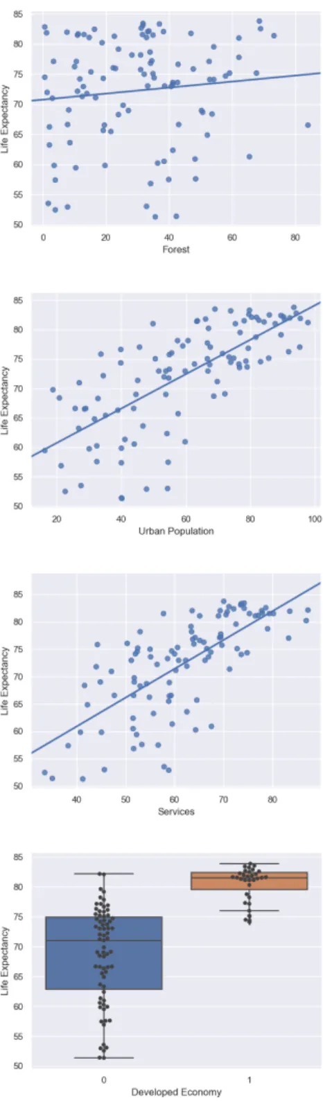
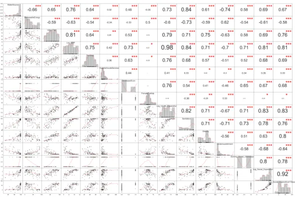
2. Investigation of the Data

The data set consists of fourteen quantitative variables and one categorical variable (Developed Economy).

(4)

(5)

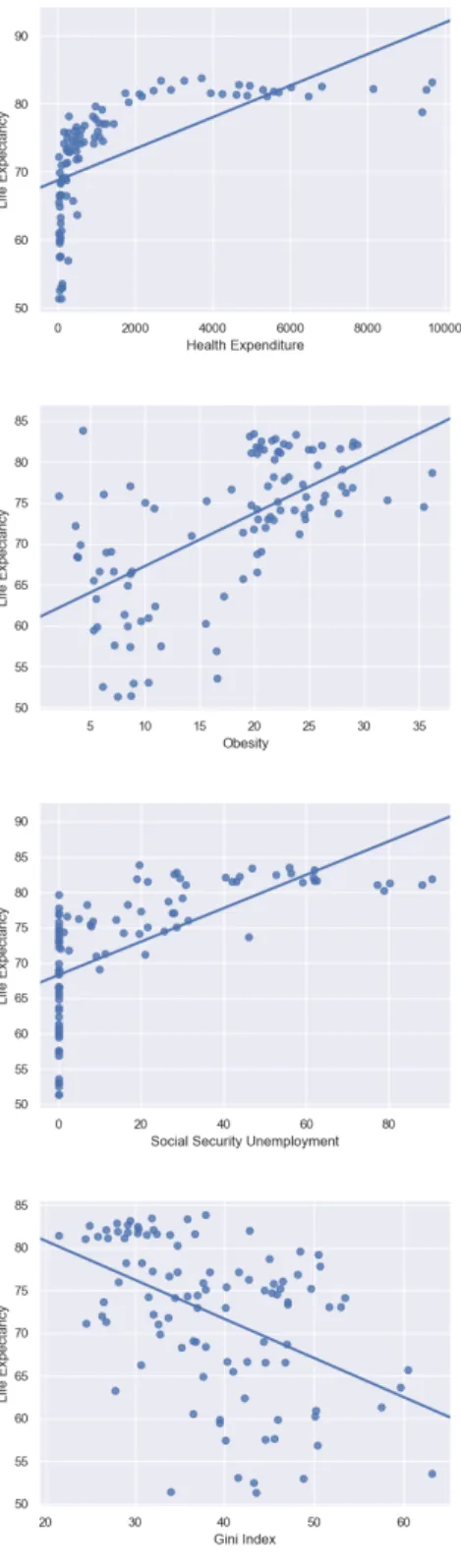
Based on the investigation of the data, we can see a non-linear relationship between Life Expectancy and some of the variables. Therefore, a preliminary transformation for the following variables is needed: GDP, Health Expenditure, Social Security Unemployment, and Social Expenditure.

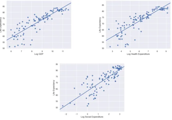
As the trend in GDP, Health Expenditure, and Social Expenditure follows the log pattern, the logarithmic transformation was perform. Since the data of Social Security Unemployment contains “0” value, we have to find a diﬀerent way from the log transformation to manage this predictor. One of the methods is to change this quantitative variable into a qualitative one (“0” when there is no social security unemployment, “1” otherwise).

Figure 2.2 Transformation of social security unemployment into a dummy variable

(6)

3. Specification of the Model

Based on Figure 2.1, we can see that no relationship occurs between Life Expectancy and Forest. Therefore, we do not include this predictor in our model. The following regressors will constitute the preliminary model:

Improved water source

Renewable energy consumption Urban population

log GDP per capita Services value added

Exports of goods and services Developed economies

Female labor force participation rate Log health expenditure per capita

Improved sanitation facilities Obesity

Undernourishment

Social security unemployment Log social protection expenditure

I have decided to add the interaction to the model : Obesity and Log social protection expenditure.

Model assumptions:

1. The mean of response is a linear function of the 2. The errors are independent

3. The errors are normally distributed

4. The errors have equal variance and mean zero x1 :

x2 :

x3 :

x4:

x5:

x6:

x7:

x8:

x9 :

x10:

x11:

x12:

x13:

x14:

yi=β0+β1xi1+β2xi2+β3xi3+β4logxi4+β5xi5+β6xi6+β7xi7+β8xi8+β9logxi9+β10xi10+ +β11xi11+β12xi12+β13xi13+β14logxi14+β15x11×logx14+ϵi

i = 1,...,n

(7)

4. Estimation of the Appropriate Model

Test for significance of Regression:

for at least one

p-value=0.000 <

We reject the null hypothesis. We can conclude that there is a statistically significant linear association between the life expectancy at birth and at least one of our predictor variables.

The prediction equation is: H0 :β1= . . . =β15= 0

H1:βj≠0 j

F0 = 47.15

α = 0.05

̂

y = 40.112882 + 0.0048x₁−0.028468x₂+ 0.014056x₃+ 2.670223logx₄+ 0.025143x₅−0.01332x₆

+0.641884x7+ 0.060922x8−1.095392logx9+ 0.182292x10−0.275188x11−0.007768x12 −2.267975x13+ 0.839871logx14+ 0.06638x11×logx14

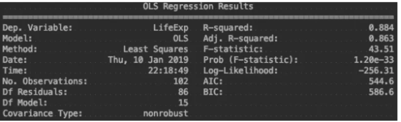
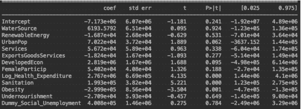
Table 4.1 OLE regression results

(8)

It appears from this analysis that only four following predictors are significant ( ): • Log GDP

• Female labor force participation rate • Sanitation

• Obesity

This preliminary model explains 88% (R-Square=0.884) of variations in the life expectancy at birth. However, further tests of model adequacy are required. Moreover, from the investigation stage, we can presume that some of the estimated coeﬀicients can be inflated by the existence of correlation among predictor variables (e.g. relationship between GDP and Health expenditure per capita).

5. Assessment of the Chosen Prediction Equation

The Breusch-Pagan test for constancy of error variance:

(constant variance)

for at least one (non constant variance) P-value=0.001 <

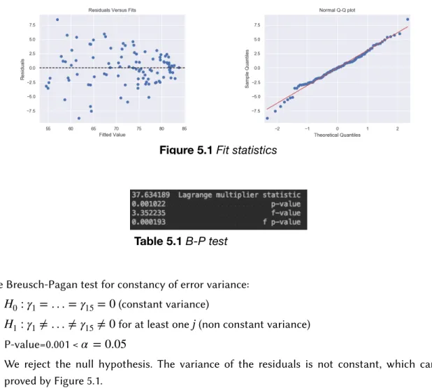
We reject the null hypothesis. The variance of the residuals is not constant, which can be also proved by Figure 5.1.

Since the variance of the residuals is not constant, we should consider the transformation of Y values. The Box-Cox analysis suggests , but we will continue with . 

α = 0.05

H0 :γ1 = . . . =γ15= 0

H1:γ1≠. . . ≠γ15≠0 j α = 0.05

λ = 3.88 λ = 4

Table 5.1B-P test

(9)

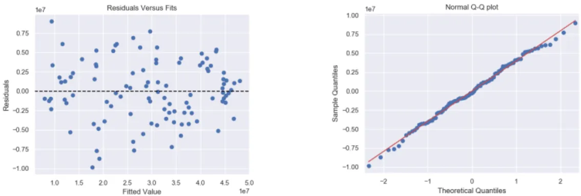
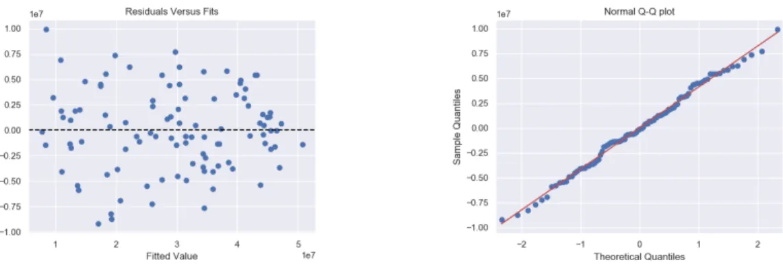
Figure 5.2 presents the fit diagnostics after the Box-Cox transformation. We can see that variance of the residuals has been improved. Normality has been also improved.

The Breusch-Pagan test for constancy of error variance: after the Box-Cox transformation:

(constant variance)

for at least one (non constant variance) P-value=0.06 >

We fail to reject the null hypothesis. The variance of the residuals is constant.

We use the Shapiro-Wilk test for normality. the errors follow a normal distribution the errors do not follow a normal distribution

P-value = 0.918 > . We fail to reject the null hypothesis. The errors follow a normal distribution. 

H0 :γ1 = . . . =γ15= 0

H1:γ1≠. . . ≠γ15≠0 j α = 0.05

H0 :

H1:

α = 0.05

Figure 5.2 Fit Statistics after the Box-Cox transformation

(10)

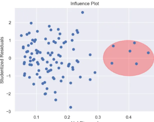
6. Outliers Diagnostics

Figure 6.1 Influence plot: studentized residuals vs. hat diagonal

Figure 6.2 Influence plot: Cook’s distance vs. DFFITS

Measure Criteria Observations

Outlier |R|>3 none

six observations none

|DFFITS| six observations

D

_i

2 p

n

= 0.314

h

_ii

2 p

n

= 0.792

4

(11)

7. Multicollinearity Diagnostics

Coeﬀicients for Log GDP, LogHealth Expenditure and the interaction Log Social Expenditure & Obesity are highly inflated.

Table 7.1 Variance inflation factor

(12)

Based on the multicollinearity diagnostics, the following predictor have been removed: • Log Social Expenditure & Obesity interaction

• Log GDP

• Log Social Expenditure

After the changes, the model includes the following variables:

• Improved water source, Renewable Energy, Urban Population, Services, Export Goods and Services, Developed Economy, Female Labor force participation rate, Log Health Expenditure, Sanitation, Obesity, Undernourishment, Dummy Social Unemployment

P-value = 0.806 > . We fail to reject the null hypothesis. The errors follow a normal distribution.

Based on Figure 7.2 and the Shapiro-Wilk test, we can conclude that the new model meets assumptions about constant variance and normality.

H0 :

H1:

α = 0.05

(13)

8. Selection of Variable Subset

With , there are three following significant predictors:

• Log health expenditure

• Improved sanitation facilities

• Obesity

With , there are five following significant predictors:

• Obesity

• Urban population

• Developed Economies

After the statistical analysis the final model includes:

• Obesity

• Urban population

• Developed Economies  α = 0.05

α = 0.1

Table 8.1 Parameter estimates after multicollinearity diagnostics

(14)

With , all regressors are significant.

, which means that 89% of variation in the life expectancy at birth is explained by the model.

The Breusch-Pagan test for constancy of error variance: after the Box-Cox transformation:

(constant variance)

for at least one (non constant variance) P-value=0.057 >

We fail to reject the null hypothesis. The variance of the residuals is constant.

α = 0.1 R2_{= 0.889}

H0 :γ1 = . . . =γ6= 0

H1:γ1≠. . . ≠γ6 ≠0 j α = 0.05

Table 8.3 Parameter estimates: model after variable selection

Figure 8.1 Fit diagnostics for a model after variable selection

(15)

P-value = 0.988 > . We fail to reject the null hypothesis. The errors follow a normal distribution.

Based on Figure 8.1, B-P test and the Shapiro-Wilk test, we can conclude that the model meets assumptions about constant variance and normality.

H0 :

H1:

(16)

9. Validation of the Regression Model

In order to validate the regression model, the dataset has been split into training (70%) and test (30%) sets.

The sum of squares of the prediction errors is

The corrected sum of squares of the responses in the prediction data set is:

and the approximate for the prediction is:

We may expect this model to explain about 97% of the variability in new data. 

(Life Expectancy)4=−4131028.131 + 76916.976×Urban Population+ 3471361.93×Developed Economy+

3010507.008×Log Health Expenditure+ 180000.231×Sanitation−192791.29×Obesity

∑ei2 =

SST =_∑yi2− (∑yi) 2

n =

R2

pred= 1− ∑e

2 i SST =

(17)

10. Conclusions

Research Question: What is the expected life expectancy at birth for a country where:

• Urban Population (in%): 34.277

• Developed Economy: 0

• Health Expenditure per capita (in USD): 30.833 (Log transformation needed: Log(30.833))

• Improved sanitation facilities (% of population with access):60.6

• Obesity (in %): 3.6

(Life Expectancy)4=−4131028.131 + 76916.976×Urban Population+ 3471361.93×Developed Economy+

3010507.008×Log Health Expenditure+ 180000.231×Sanitation−192791.29×Obesity

(Life Expectancy)4 = 19041250