This paper must be cited as:
The final publication is available at
Copyright
Additional Information
http://dx.doi.org/10.1111/j.1558-5646.2011.01451.x
http://hdl.handle.net/10251/67536
Wiley
Macia, J.; Sole, R.; Elena Fito, SF. (2012). The causes of epistasis in genetic networks.
Evolution. 66(2):586-596. doi:10.1111/j.1558-5646.2011.01451.x.
THE CAUSES OF EPISTASIS IN GENETIC NETWORKS
Javier Macía,1,2 Ricard V. Solé,1,2,3 and Santiago F. Elena3,4,5
1Complex Systems Laboratory, ICREA-Universitat Pompeu Fabra, 08003 Barcelona, Spain 2Instituto de Biología Evolutiva, CSIC-Universitat Pompeu Fabra, 08003 Barcelona, Spain 3The Santa Fe Institute, Santa Fe, New Mexico 87501, USA
4Instituto de Biología Molecular y Celular de Plantas, CSIC-Universidad Politécnica de Valencia, 46022 València, Spain.
Epistasis refers to the non-additive interactions between genes in determining phenotypes. Considerable efforts have shown that, even for a given organism, epistasis may vary both in intensity and sign. Recent comparative studies supported that the overall sign of epistasis switches from positive to negative as the complexity of an organism increases, and it has been hypothesized that this change shall be a consequence of the underlying gene network properties. Why should this be the case? What characteristics of genetic networks determine the sign of epistasis? Here we show, by evolving genetic networks that differ in their complexity and robustness against perturbations but that perform the same tasks, that robustness increased with complexity and that epistasis was positive for small non-robust networks but negative for large robust ones. Our results indicate that robustness and negative epistasis emerge as a consequence of the existence of redundant elements in regulatory structures of genetic networks and that the correlation between complexity and epistasis is a byproduct of such redundancy, allowing for the decoupling of epistasis from the underlying network complexity.
RUNNING TITLE: On the origin of epistasis
Introduction
The word epistasis was first used by Bateson (1909) to describe the masking effect that an allele (the modifier) may exert in another allele at a different locus. Later, Fisher (1918) undertook the quantitative measurement of epistasis and extended the use of this term to refer to the departure of the interaction of genetic effects of alleles on phenotypes from additivity or multiplicativity (Cordell 2002; Crow 2010). Fisher’s definition of epistasis is closer to the concept of statistical independence: departure from a specific linear model describing the relationship between variables. This definition is the one adopted by quantitative and evolutionary geneticists. Conversely, epistasis in Bateson’s sense is similar to the concept that most molecular biologists and biochemists use when investigating biological interactions between proteins. Statistical deviations from gene additivity (or multiplicativity) result from many different underlying molecular mechanisms (e.g., protein-protein interactions, dominance, associations through metabolic or regulatory networks…). Broadly speaking, epistasis is the interaction between genes in determining phenotypic traits. The direction, magnitude and prevalence of epistasis is central to theories seeking to explain the origin of genetic systems, such as sex and recombination (De Visser and Elena 2007), dominance (Bagheri and Wagner 2004), ploidy (Kondrashov and Crow 1991), robustness (De Visser et al. 2003), the ruggedness of adaptive landscapes (Weinreich et al. 2006; Poelwijk et al. 2007), or attempting to mechanistically explain dynamical biological processes such as the accumulation of mutations in finite populations (Kondrashov 1994) or speciation by reproductive isolation (Coyne 1992). All these theories provide a good knowledge about the evolutionary consequences of epistasis.
Epistasis in fitness, ε, is commonly defined as the difference between the fitness measured for a genotype carrying n ≥ 2 deleterious mutations, W1,…i,…n, and the expectation
resulting from combining the fitness measured for genotypes carrying single deleterious mutation, j, Wj: . With this definition, epistasis is said to be positive or antagonistic if ε > 0, hence the fitness observed for the multiple mutant is larger than
€
ε1,...,i,...,n=W1,...,i,...,n− Wj j=1
n
∏
expected. By contrast, epistasis is negative or synergistic if ε < 0, with the genotype carrying multiple mutations being therefore less fit than expected. A lack of epistasis would result in ε = 0.
In spite of considerable efforts, our understanding of epistasis remains fragmented mainly for two reasons. First, empirical results have been contradictory: while some support a predominance of positive epistasis (Bonhoeffer et al. 2004; Sanjuán et al. 2004; He et al. 2010), others found epistasis to be on average negative (De Visser et al. 1997a; Whitlock and Bourguet 2000; Parera et al. 2009) and some other studies suggested the lack of overall tendency for epistasis (De Visser et al. 1997b; Elena and Lenski 1997). Comparison of epistasis estimated across multiple species have shown, however, that epistasis correlates negatively with organismal complexity —complexity understood as genome size (Sanjuán and Elena 2006; Sanjuán and Nebot 2008). Accordingly, simpler organisms, such as viruses, would be dominated by positive epistasis; organisms with intermediate complexity, such as bacteria and unicellular eukaryotes, would show no overall tendency and negative epistasis would be common in more complex ones, such as fungi or flies. Second, very little is known about the evolutionary causes of epistasis, in particular about the evolutionary forces shaping the sign and intensity of epistasis in different organisms.
It has been predicted that fitness traits can evolve to be robust to genetic perturbations (Wagner et al. 1997; De Visser et al. 2003; Yuilevich et al. 2008). Indeed, several simulation studies have shown that complex evolved systems are more robust than simpler ones (Lenski et al. 1999; Azevedo et al. 2006; Macía and Solé 2009) and that a strong correlation exists between robustness and epistasis (Wilke and Adami 2001). This correlation has been experimentally confirmed by in vitro evolution experiments of the TEM-1 β-lactamase (Bershtein et al. 2006) as well as by in vivo mutation-accumulation experiments using the plant RNA virus Tobacco etch potyvirus (De la Iglesia and Elena 2007). In both examples, positive epistasis appear associated to more brittle organisms whereas more robust organisms were more prone to show negative epistases on average. Two possible explanations have been brought forward to explain
why complex biological systems are more robust than simpler ones: structural and/or functional redundancy and distributed robustness (Wagner 2005; Sanjuán and Nebot 2008), also known as degeneracy (Tononi et al. 1999). Redundancy means that elements in a genetic network are repeated, hence removing one of them has little or no effect on the network overall function (Wagner 2005), whereas degeneracy, aka distributed robustness, compares the average information shared between every possible subset of elements in the network and the rest of the network (Tononi et al. 1999). The perturbations induced by removing elements in highly degenerated networks can be buffered by the rest of the network due to the overlap in the information transferred between the different network’s subsets. Accordingly, distributed robustness arises as a consequence of the network’s architecture and connectivity (Barkai and Leibler 1997; Albert et al. 2000; Aldana and Cluzel 2003; Wagner 2005; Sanjuán and Nebot 2008): a high connectivity between components re-distributes the flux of information along alternative routes bypassing the missing or damaged nodes. Other mechanisms, such as the impact of feed-forward loops (FFL) and positive feedback loops (FBL) also seem to increase robustness (Barabási et al. 2004). FFLs are ubiquitous in Escherichia coli, yeast and other organisms and appear in systems involved in detection, sign amplification or generation of pulses, among many others (Alon 2007). FBLs involve at least two transcriptional interactions and can regulate or are regulated by other signals, including transcription cascades (Alon 2007).
Despite both theoretical and experimental advances, some pivotal questions have not been answered yet: what type of epistasis, if any, evolves in genetic networks as they become more complex? Is the observed relationship between robustness and epistasis causal or a spurious consequence of correlations with other factors? Can specific network structures, e.g., FFL and FBLs, favor some types of epistasis? What selective pressures determine the evolution of epistasis? To tackle these questions, we have evolved in silico genetic regulatory networks of variable complexity.
NETWORK IMPLEMENTATION, FITNESS AND ROBUSTNESS
Our networks start from an arbitrary number of randomly wired nodes (Figs. 1a). A network is defined as a set of nodes wired through a set of directed links Aij defining a matrix
.
(1)
Here Aij indicates a directed regulatory interaction from node Gj to node Gi. These links can be activators (Aij = 1) or inhibitors (Aij = −1) (Fig. 1b); Aij = 0 if there is no regulatory effect. These
networks will be used to implement a certain P-input, Q-output target binary function h described as a mapping:
. (2)
The network is composed by three subsets: (a) an input layer formed by P elements, (b) a hidden core and (c) an output layer formed by Q elements. Here we consider two different types of networks: those containing both FFL and FBLs (hereafter FBL-containing networks) and those that contain FFLs but not FBLs (hereafter FBL-free networks). In the case FBL-free networks there are some restrictions in the connections: (i) the P elements of the input layer can be connected either with any element of the hidden layer or the output layer, (ii) the elements of the hidden layer cannot be connected with the input layer but can be connected with the output layer, and (iii) the Q elements of the output layer can neither be connected with the hidden or input layers. There are, however, no restrictions of connections for FBL-containing networks, with the exception of those elements of the input layer that cannot be affected by the rest —i.e., cannot receive connections from other elements.
For a given input set , a given output is expected, . Here, a threshold network is defined as a set of discrete equations, where the state of each gene, indicated as , will be updated as follows:
A
=
A
11A
12...
A
1nA
21A
22...
A
2n...
...
...
...
A
n1A
n2...
A
nn!
"
#
#
#
#
#
$
%
&
&
&
&
&
h: {0,1}P
→{0,1}Q
I∈{0,1}P O(I)
∈{0,1}Q
.
(3)
In this equation, θi determines the activation internal threshold value (Fig. 1c). The gene expression pattern of a network is evaluated as follows. The network is fed with the input set I and initiates an iterative process in which the states of each node are evaluated according to equation (3). Three outcomes are then possible. First, a stable equilibrium is reached and the states of each node remain invariable, with the output set O being then recorded. Second, no equilibrium is reached and the network shows an oscillatory behavior. If this was so, we check whether the output set O is stable despite oscillations, in which case we would record its value. Third, if the output oscillates we assign zero computational efficiency (see below) to the network.
We are particularly interested in analyzing the presence of two conflicting constraints, namely the cost of continuously adding and wiring more elements into a network and the robustness against perturbations of single nodes. To evaluate how both the cost of wiring and robustness determine the performance of the networks, the following fitness function has been implemented:
. (4)
Here, fC is the computational efficiency —that is, the reliability of the gene expression pattern, measured as the distance between the output set O implemented by the circuit and its expected value. It is defined as:
. (5)
The term L is the wiring density,
, (6)
where Ω is the number of wires, and n is the number of nodes. Finally, ρ denotes the robustness of the gene expression pattern against perturbations of single nodes. Perturbations are
S
i(t
+
1)
=
1
if
A
ijS
j(t)
−θ
i>
0
j∑
0
if
A
ijS
j(t)
−θ
i≤
0
j∑
$
%
&
&
'
&
&
W= fc"#µ
(
1−L)
+(
1−µ)
ρ$%fC =1− 1
2PQ i=1 Oi−Ei 2PQ
∑
introduced knocking out each gene (i.e., fixing its state to zero). Robustness ρ is defined as the average distance between the outputs generated with (Oxi) and without (Oi) perturbations in the xth node, as follows:
.
(7) The contribution of each constraint (wiring cost and robustness) to the fitness function W is determined by . Circuits with µ = 0 pay no cost to being densely wired and have maximum robustness, whereas circuits with µ = 1 pay maximum penalty to wiring and robustness is not required. The idea here is to see the different properties of circuits that just correctly perform the desired computation but with different contributions of wiring density and robustness to their fitness. The target functions h are chosen at random: the set of outputs for each input combination are generated using 0 and 1 with equal probabilities.
The definition of fitness function given in equation (4) is, obviously, arbitrary. In principle, we shall be able to define other fitness functions that might, for instance, penalize the number of nodes instead of the number of links. Equation (4) only represents a convenient mathematical approximation to the cost of growing network complexity.
In spite of them being a toy model of gene regulation, variants of such a model have been used to study the evolution of gene network robustness (Wagner 1996) and innovation (Siegal and Bergman 2002; Ciliberti et al. 2007).
THE EVOLUTION ALGORITHM
The steps in the algorithm are:
1. Create a random generated population formed by Z individuals (candidate networks) {Γ1, ..., Γz}. Each of these individuals is formed by m randomly wired nodes (m < n) (Fig. 1b). In our simulations, all circuits start with m = 9 nodes. The wire Aij connecting a pair of nodes (Gi, Gj) can define an activator or inhibitory interaction. This population constitutes the starting generation. Here, given the computational constraints, population size at every time is Z = 100.
ρ
=
1
−
1
2
PQn
i=1O
i−
O
xi2PQ
∑
x=1 n
∑
2. The performance of each individual solution is calculated upon the 2P possible inputs according to equation (4).
3. Each individual can pass to the next generation with a probability proportional to its W value. 4. In each generation the individuals can be randomly mutated. The random mutations can be: (i) elimination of an existing connection, with probability Ec, (ii) origination of a new connection with probability Cc, (iii) elimination of a node with probability In, (iv) origination of a new node with probability Cn, (v) duplication of a node and its connections with probability Dn, (vi) changes in the type of interaction between two links, i.e. changes from Aij = 1 to Aij = −1 or vice versa with probability CA, and (vii) mutations in the values of the internal threshold θi with probability Cθ. The mutations can increase or decrease θi in a random amount according to the following equation:
(8) where g is the generation number and .
We performed multiple experiments with different values of parameters and no relevant qualitative changes were observed. Here we used P = 3, Q = 1, Ec = 0.01, Cc = 0.03, In = 0.01, Cn = 0.01, Dn = 0.03, CA = 0.02, Cθ = 0.03, and τ = 0.01. Step 2 was repeated until W reached a stable value. In our experiments we consider that the network has reached a stable performance if no changes in W were observed during 1000 generations.
EPISTASIS MEASUREMENTS
The average epistasis of the networks upon two nodes perturbed once can be calculated as:
ε = 1
n2
(
fC,xy−fC,xfC,y)
y=x+1 n∑
x=1 n−1∑
, (9) where (x, y) represents the set of all possible n(n – 1)/2 pairs of different nodes x and y. Here fC,xy is the computational efficiency (i.e., gene expression dynamics) upon knocking out nodes x and y simultaneously, whereas fC,x and fC,y are the efficiencies calculated perturbing a single node x or y, respectively. These efficiencies were evaluated using the following two modifications of equation (5):θi(g+1)=θi(g)(1+η) η∈{−τ,+τ}
(10) and
(11) where Oi if the output generated by the unperturbed network in response to the ith input combination, Oxi is the output after a single perturbation of the node x, and Oxyi denotes the output resulting from simultaneously perturbing nodes x and y.
Comparison of equations (7) and (10) shows that robustness can be also computed as
ρ=1−1
nx=1
(
1−fC,x)
=1− s n∑
, where 〈s〉 is the average fitness effect associated to individualmutations: the smaller the average effect of mutations on the computational ability of networks, the more robust they are and vice versa.
MEASURES OF REDUNDANCY, DEGENERACY AND COMPLEXITY
The analysis of the factors affecting the network-level properties of an evolved biological system requires reliable quantitative measures. Such measures must capture the presence of two relevant components of network complexity: modularity and integration. Modularity refers to the existence of subparts of the system that are isolated or semi-isolated and typically perform well-defined functions. They are thus network modules, observed as segregated subsets within the system. In an ideal scenario, a module performs a given, specialized function. In order to have redundant behaviour, similar modules will perform identical functions. Isolation therefore favours redundancy. Integration, is required when different types of information need to be combined to generate a given response. A highly integrated system will not be modular, since most parts of the system will receive inputs from (and send outputs to) other parts. In general terms, the higher the integration the less likely that two different parts will behave in the same way and, thus, the less the redundancy will be. Real systems seem to be somewhat in an intermediate position between full modularity and complete integration, an expected solution for a system in which robust behaviour is the consequence of degeneracy (i.e., distributed
fC,x=1− 1
2PQ i=1 Oi−Oxi 2PQ
∑
fC,xy=1− 1
2PQ i=1 Oi−Oxyi 2PQ
robustness) rather than being due to the presence of redundant parts. The complexity of the two extremes is low, since independent modules limit information processing whereas highly connected components fail to perform specialized tasks. The measure of complexity presented below weights properly the contribution of modularity versus integration. From the point of view of dynamical responses and their control, it also provides a measure of the degree of information integration displayed by subsets of different sizes. A system able of processing and storing information will have a high (computational) complexity. Such trade-offs are consistently captured by information theory-based measures of network redundancy, degeneracy and complexity (Tononi et al. 1999).
The basic measure of information theory is entropy (Ash 1990)
(12) for one single variable x, and
(13) for two variables x and y. Here, p(x) is the probability distribution for all possible values of x and p(x, y) is the joint probability distribution. Using these measures, it is possible to define the mutual information M(X, Y) as
. (14)
M measures the information transmitted through the network. Considering networks formed by n nodes Si and the output layer O, redundancy R(S;O) can be defined as
, (15)
where M(Si;O) represents the mutual information between a given node Si and the output layer O. According to this definition, R(S;O) = 0 if all Si elements contribute to the output O independently and hence mutual information between the entire network and the output layer equals the sum of the mutual information for all the nodes. Contrary to this, R(S;O) is high if the sum of the mutual information content in the link between each node Si and Ois larger than that between the entire network and O, indicating that each node of the network contributes with similar information with respect to the output.
The degeneracy of a network can be defined as
H(X)=− p(x)log(x)
x
∑
∈XH(X,Y)=− p(x,y)log(x,y) y∈Y
∑
x
∑
∈XM(X,Y)=H(X)+H(Y)−H(X,Y)
R(S;O)=
[
M(Si;O)]
−M(S;O) i=1n
. (16) where M(Si;S − Si;O) = M(Si;O) + M(S − Si;O) − M(S;O). Here M(S − Si;O) represents the
mutual information content between the rest of the network (excluding the node Si) and O. In this case, the measure accounts for the overlap in mutual information between each element Si and O with respect to the mutual information between the rest of the system S−Si and O that
cannot be explained due to the existence of redundancy.
Finally, Edelman’s complexity can be defined in terms of entropy between Si, S−Si and
the output layer O according with
. (17)
Note that C(S) = 0 for systems composed of disconnected elements, takes low values for systems composed by nodes that are integrated and homogeneous (undifferentiated) and high values for systems that are both integrated and differentiated.
Results and Discussion
EVOLUTION OF NETWORKS OF VARYING COMPLEXITY
To achieve the required variation in complexity, we evolved asexual populations of regulatory networks starting from an arbitrary number of randomly wired nodes under the simple mutation-selection rules described in the Methods section. At each evolutionary step, networks can mutate by adding or removing nodes and links and the performance of each network in the population can be evaluated using the fitness function defined by equation (4) that accounts for the relative contributions of wiring and robustness. In this equation, the tuning parameter µ
allows to favor robust networks without imposing a cost to their size and wiring density (µ→ 0)
or to favor small and sparsely wired networks with no robustness (µ → 1). In all cases,
regardless these constraints, all networks had to optimize its computational fitness fC. After a number of generations, several key quantities can be characterized, including average degree connectivity (〈K〉), Edelman’s complexity (C; equation (17)), average epistasis for all possible
pairs of knockouts (〈ε〉; equation (9)), computational robustness (ρ; equation (7)), degeneracy
D(S;O)=
[
M(Si;S−Si;O)]
−R(S;O) i=1n
∑
C
(
S
)
=
H
(
S
)
−
[
H
(
S
i;
S
−
S
i)
−
H
(
S
−
S
i)
]
i=1
n
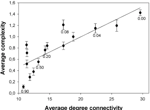
(D; equation (16)) and redundancy (R; equation (15)). Reported values are averages for networks evolved at each given µ. The evolved networks varied widely in complexity. 〈K〉
ranged between 10 and 30 links per node, the total number of links per network varied between 50 and 500, and the number of nodes ranged between 10 and 30. Since 〈K〉 and Edelman’s C
complexity shows a highly significant positive correlation (Fig. 2; Pearson’s r = 0.8331, 13 d.f., P = 0.0001), therein we will only report results based in C measure. Here C weights the functional tradeoffs between integration and modularity of a given dynamical network. It thus captures the functional organization of the system as a whole. Moreover, to test whether FBLs were responsible for ρ and 〈ε〉, we performed a second evolution experiment in which a new set
of networks was generated avoiding the formation of FBLs (FBL-free networks) while still retaining FFLs (FBL-containing networks).
As expected, when µ was small, the resulting networks had high complexities, whereas
for large µvaluesnetworks were much simpler (r = –0.9133, 13 d.f., P < 0.0001). In particular,
complex networks also contained more and larger FBLs than simple ones, even after adjusting for differences in the total number of links (partial r = –0.7746, 12 d.f., P = 0.0011) and nodes (partial r = –0.8766, 12 d.f., P < 0.0001) on each type of network.
NETWORK COMPLEXITY AND THE DISTRIBUTIONS OF MUTATIONAL FITNESS EFFECTS
The analysis of epistasis relies on the assumption that mutations are either deleterious or beneficial. A balanced mixture of both types of mutations may be problematic because the direction of epistasis between a deleterious and a beneficial mutation cannot be interpreted in the same way as the combination of deleterious or beneficial mutations. Therefore, for each evolved network, we evaluated the fitness effect (sx = 1 − fC,x, where fC,x was computed using
equation (10)) of each possible knockout mutation. Mutations were always neutral (sx = 0) or deleterious (sx > 0), with no mutation showing a beneficial effect, thus eliminating the possibility of confounding effects when evaluating epistases. Table 1 shows the statistics
characterizing the distribution of mutational effects for networks obtained at increasing values of the tuning parameter µ. As expected, the average deleterious effects 〈s〉 of knockout
mutations became significantly stronger as µ increased, reflecting the relaxation for
computational robustness imposed by equation (18). This conclusion holds both for FBL-containing (r = 0.8283, 9 d.f., P = 0.0016) and for FBL-free (r = 0.6347, 9 d.f., P = 0.0359) networks. Using median deleterious effects, however, which are less affected by the asymmetry of the distribution of mutational effects, the conclusion holds for FBL-containing networks (r = 0.6482, 9 d.f., P = 0.0310), but not for FBL-free networks (r = 0.3252, 9 d.f., P = 0.2876). Mutational effects were, on average, stronger for FBL-containing than for FBL-free networks (ANOVA using µ as covariable: F2,19 = 62.3715, P < 0.0001). This result was reproduced when
median values were used instead of average values. In general, distributions of mutational effects were right-skewed, indicating a relatively low number of large effect mutations, and platykurtic (negative kurtosis), as corresponds to distributions with a lower and wider peak around the mean relative to the Gaussian distribution. None of these shape parameters changed with increasing µ (in all cases, P ≥ 0.0632). By contrast, the standard deviation showed an
increasing trend with µ for both types of networks (FBL-containing: r = 0.9262, 9 d.f., P <
0.0001; FBL-free: r = 0.8088, 9 d.f., P = 0.0026). Finally, the frequency of neutral mutations was insensitive to changes in µfor FBL-containing networks (r = −0.1992, 9 d.f., P = 0.5570)
but significantly increased for FBL-free networks (r = 0.6341, 9 d.f., P = 0.0362).
ASSOCIATION BETWEEN COMPLEXITY AND EPISTASIS
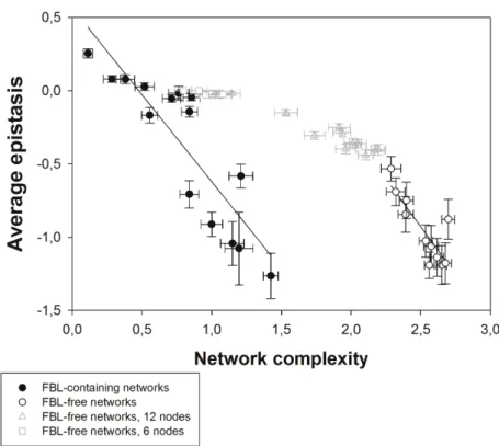
After generating the collection of networks of varying complexity, we sought for an association between C and 〈ε〉. As Figure 3 shows, these two variables are negatively associated for
FBL-containing networks (r = –0.9747, 13 d.f., P < 0.0001) such that the dominant type of epistasis on more complex networks is negative whereas positive epistasis is the hallmark of simple networks. The sign of epistasis depends on how nodes in the network interact to complete computations. If each of the n nodes is necessary for the right computation and, in the extent to
which fitness disadvantage created by carrying a given number of mutations would be similar to that of each single mutant, epistasis should be positive (Sanjuán and Elena 2006). In general, positive epistasis should take place in small networks with few nodes because multiple mutations will often hit essential bits of the same functional module (Sanjuán and Nebot 2008). By contrast, if each of the n nodes in the network is sufficient for computation, epistasis should be negative, because networks carrying an arbitrary number of mutations would be disproportionally worse than the effect of each mutation independently. Conversely to this, FBL-free networks have a similar negative correlation between C and 〈ε〉 (Fig. 3: r = –0.8326, 9
d.f., P = 0.0015) but 〈ε〉 is always negative. Interestingly, FBL-free networks exhibit higher
complexity values indicating that networks can overcome the imposed topological constraints by increasing their informational complexity in response to the selective pressure to increase robustness. These results indicate that evolved networks show a negative correlation between
〈ε〉 and C but this correlation is dependent on topological constraints, although the topological
constraints do not change the underlying relationship between epistasis and complexity (test of parallelism among regression lines: t22 = 0.0556, P = 0.8157). In other words, there is no univocal association between C and 〈ε〉 because it is possible to find networks with similar
values of average epistasis but with different levels of complexity. To test whether a reduction in complexity is associated to an increase in average epistasis we have evolved a set of FBL-free networks constraining the number of nodes to either 12 or six (Fig. 3). In spite of the difficulty in optimizing the computational fitness fC for this case, evolved networks present a clear reduction in complexity that correlates with an increase in epistasis (Fig. 3), showing a tendency in agreement with the results obtained in FBL-containing networks.
RELATIONSHIP BETWEEN EPISTASIS AND ROBUSTNESS
It has been postulated that epistasis and robustness are two sides of the same coin and that negative epistasis must be a hallmark of robustness (Proulx and Phillips 2005; Bershtein et al. 2006; Sanjuán and Elena 2006; Desai et al. 2007). In the light of this, robustness is the real
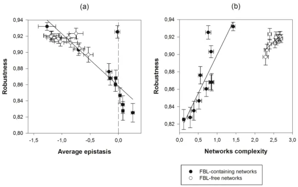
target of selection, while negative epistasis should be a byproduct of robustness (Azevedo et al. 2006). We aimed to test this prediction on our set of evolved networks. Since we evolved networks that varied in their robustness without imposing any direct selective pressure on epistasis, we sought for whether the predicted correlation could arise in our networks. Figure 4a confirms that the relationship between 〈ε〉 and ρ is univocal and highly significant (r = –0.8569, 20 d.f., P < 0.0001), regardless whether or not networks contained FBLs. This relationship, that confirms previous results (Wilke and Adami 2001; Bershtein et al. 2006; De la Iglesia and Elena 2007), implies that negative epistasis is associated to robust networks, whereas robustness decreases as epistasis switches to positive sign. Accordingly, the more negative epistasis values corresponded, on average, to pairs of two neutral mutations, followed by combinations of one deleterious and one neutral mutation and, finally, by pairs of deleterious mutations, for which cases of positive epistasis were over-represented (Friedman’s test, P < 0.0001).
As expected from the results shown in the previous section, where we explored the relationship between C and 〈ε〉, ρ and C were also significantly correlated, although the relationship is not univocally determined but dependent upon topological constraints (Fig. 4b; FBL-containing networks: r = 0.8456, 9 d.f., P = 0.0010; FBL-free networks: r = 0.7284, 9 d.f., P = 0.0110), thus illustrating that two networks can attain the same robustness despite representing markedly different complexities. Regardless the strength of the topological constraints, the underlying relationship between epistasis and complexity was the same in both types of networks (test of parallelism among regression lines: t18 = 1.9045, P = 0.0730).
DISSECTING THE CAUSES OF ROBUSTNESS AND EPISTASIS
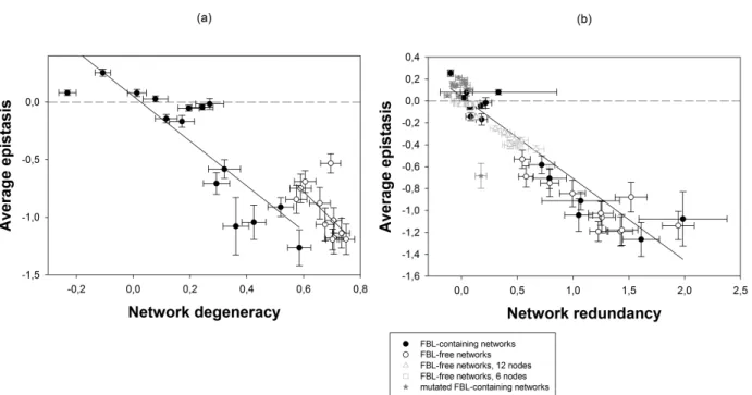
At this point the key question is: What mechanism is mainly responsible for epistasis? To elucidate this question we have analyzed the two main candidate mechanisms involved in robustness namely, degeneracy D and redundancy R. As shown in Figure 5a the relationship between 〈ε〉 and D exhibits a similar behavior that the one observed for C, allowing for
constraints (r = −0.8557, 13 df, P < 0.0001 for FBL-containing networks; r = −0.6245, 9 df, P =
0.0400 for FBL-free networks). The underlying relationship between 〈ε〉 and D remains
constant regardless whether networks may or may not contain FBLs (test of parallelism among regression lines: t22 = 0.1292, P = 0.7227).
In contrast to the previous observations, 〈ε〉 shows a strong negative correlation with R
independently on whether the resulting topology contains FBLs (Fig. 5b; overall r = −0.9286,
24 df, P < 0.0001). Therefore, negative epistasis is a consequence of redundancy, as previously suggested by Sanjuán and Elena (2006). We have further tested this conclusion by removing the FBLs from the FBL-containing networks. Even though these mutations modify the function implemented by the networks, a clear reduction of the redundancy levels was observed and consequently the epistasis increased toward positive values, while still retaining a similar negative association (Fig. 5b).
So far we have shown that epistasis relates to network complexity in a non-univocal way that depends on topological constraints. As stated above, the two mechanisms through which complex networks can achieve robustness are redundancy and degeneracy. We have also shown that only R determines epistasis univocally (Fig. 5b), whereas D does not (Fig. 5a). That is to say, given a value of redundancy, we can estimate the sign and strength of epistasis, but given a value of degeneracy we cannot do so unless additional information on topological constraints is also available. Therefore, the non-univocal relationship observed between epistasis and complexity (Fig. 3) is a consequence of the non-univocal relationship that epistasis has with degeneracy. Figure 6 shows the positive non-univocal association existing between D and C for FBL-containing and FBL-free networks (r = 0.9088, 13 df, P < 0.0001 and r = 0.5982, 9 df, P = 0.0519, respectively). Although topology elements are very different, the underlying relationship between C and D is equivalent in both sets of networks (test of parallelism among regression lines: t22 = 1.7768, P = 0.1962).
The results shown here suggest that epistasis emerges in genetic regulatory networks as a direct consequence of selection for robustness via the presence of redundant elements rather than via the increase in degeneracy (i.e., distributed robustness). The correlation between epistasis and complexity seems, however, to be a byproduct of the correlation with redundancy. Networks with different complexity and degeneracy values have similar epistasis if they also have similar degrees of redundancy. This is a striking result as robustness and epistasis have been proposed to be two intrinsically associated properties of biological systems (Lenski et al. 1999; Wilke and Adami 2001; Azevedo et al. 2006; Sanjuán and Elena 2006; De Visser and Elena 2007). Moreover, epistasis must necessarily evolve under selection for buffering the effect of mutations (Desai et al. 2007).
In this context, it has been argued that sexual reproduction creates the conditions that would favor the evolution of robustness and negative epistasis (Azevedo et al. 2006). Nonetheless, this possibility is at odds with results from a theoretical study concluding that positive epistasis should be favored in sexual populations (Desai et al. 2007). This opposing view may be ameliorated by the inherent weaknesses of the study by Desai et al. (2007), according to which robustness was not evolvable but selection operated upon epistasis. Our experimentally evolving populations overcome some of these problems: first, they were truly asexual populations and thus redundancy-based robustness emerged for reasons other than ensuring the transmission of well-tuned modules within the network and, second, selection directly operated on robustness rather than on epistasis.
ACKNOWLEDGEMENTS
We thank J. Carrera, J.A.G.M. de Visser, M.A. Fares, and S. Valverde for discussions and two anonymous reviewers for insightful suggestions. This work was supported by the Spanish Ministry of Science and Innovation grant BFU2009-06993 (SFE), the Generalitat Valenciana grant PROMETEO2010/019 (SFE), the Human Frontiers Science Program grant RGP12/2008 (SFE and RVS) and the Santa Fe Institute.
LITERATURE CITED
Albert, R., H. Jeong, and A.L. Barabási. 2000. Error and attack tolerance of complex networks. Nature 406:378-382.
Aldana, M., and P. Cluzel. 2003. A natural class of robust networks. Proc. Natl. Acad. Sci. USA 100:8710-8714.
Alon, U. 2007. Network motifs: theory and experimental approaches. Nat. Rev. Genet. 8:450-461.
Ash RB (1990) Information Theory. Dover Publications, New York, USA.
Azevedo, R.B.R., R. Lohaus, S. Srinivasan, K.K. Dang, and C.L. Burch. 2006. Sexual reproduction selects for robustness and negative epistasis in artificial gene networks. Nature 440:87-90.
Bagheri, H.C., and G.P. Wagner. 2004. Evolution of dominance in metabolic pathways. Genetics 168:1716-1735.
Barabási, A.L., and Z.N. Oltvai. 2004. Network biology: understanding the cell’s functional organization. Nat. Rev. Genet. 5:101-114.
Barkai, N., and S. Leibler. 1997. Robustness in simple biochemical networks. Nature 387:913-917.
Bateson, W. 1909. Mendel’s Principles of Heredity. Cambridge University Presss, Cambridge. Bershtein, S., M. Segal, R. Bekerman, N. Tokuriki, and D.S. Tawfik. 2006. Robustness-epistasis
link shapes the fitness landscape of a randomly drifting protein. Nature 444:929-932. Bonhoeffer, S., C. Chappey, N.T. Parkin, J.M. Whitcomb, and C.J. Petropoulos. 2004. Evidence
for positive epistasis in HIV-1. Science 306:1547-1550.
Ciliberti, S., O.C. Martin, and A. Wagner. 2007. Innovation and robustness in complex regulatory gene networks. Proc. Natl. Acad. Sci. USA 104:13591-13596.
Cordell, H.J. 2002. Epistasis: what it means, what it doesn’t mean, and statistical methods to detect it in humans. Hum. Mol. Genet. 11:2463-2468.
Coyne, J.A. 1992. Genetics and speciation.Nature 355:511-515.
Crow, J.F. 2010. On epistais: why it is unimportant in polygenic directional selection. Phil. Trans. R. Soc. B 365:1241-1244.
De la Iglesia, F., and S.F. Elena. 2007. Fitness declines in Tobacco etch virus upon serial bottlenecks transfers. J. Virol. 81:4941-4947.
De Visser J.A.G.M., J. Hermisson, G.P. Wagner, L. Ancel-Meyers, H. Bagheri-Chaichian, et al. 2003. Perspective: Evolution and detection of genetic robustness. Evolution 57:1959-1972.
De Visser, J.A.G.M., and S.F. Elena. 2007. The evolution of sex: empirical insights into the roles of epistasis and drift. Nat. Rev. Genet. 8:139-149.
De Visser, J.A.G.M., R.F. Hoekstra, and H. van den Ende. 1997a. An experimental test for synergistic epistasis and its application in Chlamydomonas. Genetics 145:815-819. ———. 1997b. Test of interaction between genetic markers that affect fitness in Aspergillus
niger. Evolution 51:1499-1505.
Desai, M.M., D. Weissman, and M.W. Feldman. 2007. Evolution can favor antagonistic epistasis. Genetics 177:1001-1010.
Elena, S.F., and R.E. Lenski. 1997. Test of synergistic interactions among deleterious mutations in bacteria. Nature 390:395-398.
Fisher, R.A. 1918. The correlation between relatives on the supposition of Mendelian inheritance. Trans. R. Soc. Edin. 52:399-433
He, X., W. Qian, Z. Wang, Y. Li, and J. Zhang. 2010. Prevalent positive epistasis in Escherichia coli and Saccharomyces cerevisiae metabolic networks. Nat. Genet. 42:272-276.
Kondrashov, A.S. 1994. Muller’s ratchet under epistatic selection.Genetics 136:1469-1473. Kondrashov, A.S., and J.F. Crow. 1991. Haploidy or diploidy: which is better.Nature
351:314-315.
Lenski, R.E., C. Ofria, T.C. Collier, and C. Adami. 1999. Genome complexity, robustness and genetic interactions in digital organisms. Nature 400:661-664.
Macía, J., and R.V. Solé. 2009. Distributed robustness in cellular networks: insights from synthetic evolved circuits. J. R. Soc. Interface 6:393-400.
Parera, M., N. Pérez-Álvarez, B. Clotet, and M.A. Martínez. 2009. Epistasis among deleterious mutations in the HIV-1 protease. J. Mol. Biol. 392:243-250.
Poelwijk, F.J., D.J. Kiviet, D.M. Weinreich, and S.J. Tans. 2007. Empirical fitness landscapes reveal accessible evolutionary paths. Nature 445:383-386.
Proulx, S.R., and P.C. Phillips. 2005. The opportunity for canalization and the evolution of genetic networks. Am. Nat. 165:147-162.
Sanjuán R., and S.F. Elena. 2006. Epistasis correlates to genome complexity. Proc. Natl. Acad. Sci. USA103:14402-14405.
Sanjuán, R., A. Moya, and S.F. Elena. 2004. The contribution of epistasis to the architecture of fitness in an RNA virus. Proc. Natl. Acad. Sci. USA 10:15376-15379.
Sanjuán, R., and M.R. Nebot. 2008. A network model for the correlation between epistasis and genomic complexity. PLoS ONE 3:e2663.
Siegal, M.L., and A. Bergman. 2002. Waddington’s canalization revisited: developmental stability and evolution. Proc. Natl. Acad. Sci. USA 99:10528-10532.
Tononi, G., O. Sporns, and G.M. Edelman. 1999. Measures of degeneracy and redundancy in biological networks. Proc. Natl. Acad. Sci. USA 96:3257-3262.
Wagner, A. 1996. Does evolutionary plasticity evolve? Evolution 50:1008-1023.
———. 2005. Distributed robustness versus redundancy as causes of mutational robustness. BioEssays 27:176-188.
Wagner, G.P., G. Booth, and H. Bagheri-Chaichian. 1997. A population genetic theory of canalization. Evolution 51:329-347.
Weinreich, D.M., N.F. Delaney, M.A. DePristo, and D.L. Hartl. 2006. Darwinian evolution can follow only very few mutational paths to fitter proteins.Science 312:111-114.
Whitlock, M.C., and D. Bourguet. 2000. Factors affecting the genetic load in Drosophila: synergistic epistasis and correlations among fitness components. Evolution 54:1654-1660.
Wilke, C.O., and C. Adami. 2001. Interaction between direction epistasis and average mutational effect. Proc. R. Soc. B 268:1469-1474.
Yukilevich, R., J. Lachance, F. Aoki, and J.R. True. 2008. Long-term adaptation of epistatic genetic networks. Evolution 62:2215-2235.
Figure 1. (a) A simple model of regulatory interactions where genes interact through both positive and negative links. (b) This simple feed-forward loop network can be mapped into a direct graph where edges have weights (A) that connect genes Gi (nodes). Here each node has a different response threshold θi. (c) Hypothetical activation function for gene G3. The threshold θ3 defines the concentration of both inputs G1 and G2 necessary for triggering the activation of G3. Si(t) represents the state of a given gene at time t (1 represents the active state and 0 the inactive one).
Figure 2. Positive association between average degree connectivity (〈K〉) and complexity (C).
The solid line is presented with the only purpose of highlighting the relationship between both variables. Error bars represent ±1 SEM calculated over all the networks evolved for the same
value of the tuning parameter µ. For illustrative purposes, a few µ values are indicated below
the corresponding data. More complex networks and connected networks evolved for smaller µ
Figure 3. Negative correlation between average epistasis (〈ε〉) and complexity (C) in evolved
genetic networks. A transition from positive to negative 〈ε〉 is observed when C increases in
FBL-containing networks. However, only negative 〈ε〉 has been observed for FBL-free
networks. In both cases the magnitude of the negative correlation is equivalent. When the increase of complexity for FBL-free networks is limited by constraining the number of possible nodes, a clear decrease in 〈ε〉 is observed, tending towards the values characteristic of
FBLs-containing networks. The horizontal dashed line represents the case of 〈ε〉 = 0. The solid lines
are presented with the only purpose of highlighting the relationship between 〈ε〉 and C. Error
bars represent ±1 SEM calculated over all the networks evolved for the same value of the tuning
Figure 4. Association between robustness (ρ) and complexity (C) and average epistasis (〈ε〉).
(a) The correlation of ρ with 〈ε〉. The vertical dashed line represents the case of 〈ε〉 = 0. (b) The
correlation of ρwith C. The solid lines are presented with the only purpose of highlighting the relationship between variables. Error bars represent ±1 SEM calculated over all the networks
Figure 5. Association between average epistasis (〈ε〉) and degeneracy (D) and redundancy (R).
(a) The correlation of 〈ε〉 with D is not univocal but depends on the network topological
constraints. (b) The correlation between 〈ε〉 and R is univocal and independent of network
constraints. To test whether a reduction in R comes with an increase in 〈ε〉, FBL-containing
networks have been mutated by removing the feedback links. The resulting networks, now only containing FFLs, show a reduction in D with a corresponding increase of 〈ε〉 but still
maintaining the same relationship. The horizontal dashed line represents the case of 〈ε〉 = 0.
The solid lines are presented with the only purpose of highlighting the relationship between variables. Error bars represent ±1 SEM calculated over all the networks evolved for the same
Figure 6. Positive correlation between degeneracy (D) and complexity (C). The differences among FBL-containing and FBL-free networks led to the differences in the correlation between average epistasis and C shown in Fig. 3, indicating that this correlation is a by-product of redundancy.
Table 1. Statistics describing the distribution of mutational fitness effects (sx) for networks evolved at increasing values of the tuning parameter µ.
µ Mean Median Std. dev. Skewness Kurtosis Neutrality
FBL-containing networks
0 0.0680 0.0650 0.0529 1.1351 3.4334 0.1417 0.1 0.0968 0.0920 0.0756 0.4689 −0.5244 0.1667
0.2 0.1320 0.1424 0.0931 0.4412 −0.3647 0.1083
0.3 0.1396 0.1458 0.0956 −0.0321 −1.1344 0.1750
0.4 0.0747 0.0477 0.0843 1.3040 1.0420 0.3083 0.5 0.1239 0.1056 0.1099 0.3579 −1.2268 0.2667
0.6 0.1319 0.1139 0.1090 0.5327 −0.6089 0.2083 0.7 0.1533 0.1500 0.1039 0.5753 0.2167 0.0917 0.8 0.1646 0.1632 0.1194 0.1389 −1.0799 0.1667
0.9 0.1747 0.1563 0.1262 0.1641 −1.1204 0.0583
1 0.1724 0.1577 0.1282 0.1832 −1.2670 0.1500
FBL-free networks
0 0.0820 0.0789 0.0488 0.2899 −0.3784 0.0440
0.1 0.0817 0.0833 0.0444 0.0144 −0.7287 0.0220
0.2 0.0792 0.0797 0.0474 0.2779 −0.3404 0.0220
0.3 0.0793 0.0774 0.0538 0.3070 −0.7337 0.0989
0.4 0.0829 0.0789 0.0584 0.8309 0.8536 0.0549 0.5 0.0869 0.0855 0.0518 0.6617 0.6779 0.0330 0.6 0.0803 0.0823 0.0600 0.5444 0.3090 0.1538 0.7 0.0880 0.0875 0.0539 0.2668 −0.3922 0.0659
0.8 0.0767 0.0641 0.0624 0.3456 −1.2288 0.1538
0.9 0.0950 0.0929 0.0635 0.3359 −0.4800 0.0440