Computer Science and Software Engineering
ISSN: 2277-128X (Volume-7, Issue-6)
2017
Deploying the Queueing Model in the Remote Patient
Medical Monitoring System
Ifeoma V. Ngonadi
Dept. of General Studies (Maths& Computer Science Unit) Petroleum Training Institute Effurun, Nigeria
DOI: 10.23956/ijarcsse/V7I6/01605
Abstract: A queueing system can be described as patients arriving for service, waiting for service if it is not immediate, utilizing the service and leaving the system after being served. The queueing model is constructed so that queue lengths and waiting time can be predicted.Remote patient monitoring enables the monitoring of patients’ vital signs outside the conventional clinical settings which may increase access to care and decrease healthcare delivery costs. This paper focuses on applying the queueing model to the remote patient medical monitoring system. This was achieved by writing a java program which adapts an M/M/1queueing model that employs the first come first serve discipline to store the patients’ medical records generated by a simulated mobile phone called the Intelligent Personal Digital Assistant according to when they arrive at the queue. The queueing model gives the summary of the total number of readings generated for each patient and also plots a graph so that the doctor can see the progression of each patient’s readings at a glance. The result of this research work produces an enhanced remote patient medical monitoring system which has the capacity to save lives.
Keywords: Queueing Model, Intelligent Personal Digital Assistant, Remote Medical Monitoring, Vital Signs, M/M/1
I. INTRODUCTION
A queueing system can be described as patients arriving for service, waiting for service if it is not immediate, utilizing the service and leaving the system after being served.
Queueing theory is the mathematical study of waiting lines, or queues[19].The queueing model is constructed so that queue lengths and waiting time can be predicted [19]. Queueing theory is generally considered a branch of operations research because the results are often used when making business decisions about the resources needed to provide a service.
Queues form when entities that request service, typically referred to as customers, arrive at a service facility and cannot be served immediately upon arrival. In healthcare delivery systems, patients are typically the customers and either outpatient clinics or diagnostic imaging centers or hospitals are the service facilities.
Single queueing nodes are usually described using Kendall's notation in the form A/S/C where A describes the time between arrivals to the queue, S the size of jobs and C the number of servers at the node [20][8]. Many theorems in queueing theory can be proved by reducing queues to mathematical systems known as Markov chains, first described by Andrey Markov in his 1906 paper [13].
The M/M/1 queue is a simple model where a single server serves jobs that arrive according to a Poisson process and have exponentially distributed service requirements. In an M/G/1 queue the G stands for general and indicates an arbitrary probability distribution. The M/G/1 model was solved by Felix Pollaczek in 1930 [17], a solution later recast in probabilistic terms by AleksandrKhinchin and now known as the Pollaczek–Khinchine formula[10][23].
Remote medical monitoring of patients requires monitoring the physiological state of patients with acute or chronic conditions or chronic disease states which predominantly derive decided prognosis advantages from intensive condition tracking. More particularly, the invention is directed to a condition monitoring system which includes one or more remote modular testing units and a central station. The remote units include physiological parameter testing modules to acquire data from one or possibly many patients and communicate with a central station typically capable of interfacing with a large number of patient-operated units or clinician-operated units testing many patients. The central station, in turn, may interface and communicate with any number of other devices as by networking. Parameters checked may include but are not limited to blood pressure, pulse rate, blood oxygen saturation, weight, blood glucose, temperature, prothrombin (clotting) time and pulmonary function, including respiratory rate and depth. Other functions, such as ECG (electrocardiograph) traces and infant breathing monitoring for detection of SIDS (sudden infant death syndrome) onset are also contemplated [15].
ISSN: 2277-128X (Volume-7, Issue-6) system are taken to assure that the right patient is being monitored, that the patient is being tested properly and that the system is being monitored appropriately.
As the vital signs of patients are monitored from different locations and sent to the server in the hospital, it is necessary to put these readings in a queue so that there will not be jamming of data. The M/M/1 queueing model which operates on the First Come First Serve (FCFS) basis is used meaning that the packets of data enter the queue according to when they arrive the queue. Java language is used to write a program for the implementation of this queuing model.
II. RELATED WORK
Queueing theory has its origins in research by AgnerKrarupErlang when he created models to describe the Copenhagen telephone exchange [19]. The ideas have since seen applications including telecommunication, traffic engineering, computing[12] and, particularly in industrial engineering, in the design of factories, shops, offices and hospitals, as well as in project management[18][14].
AgnerKrarupErlang, a Danish engineer who worked for the Copenhagen Telephone Exchange, published the first paper on what would now be called queueing theory in 1909[1][2][4]. He modeled the number of telephone calls arriving at an exchange by a Poisson process and solved the M/D/1 queue in 1917 and M/D/k queueing model in 1920[10]. In Kendall's notation:
M stands for Markov or memoryless and means arrivals occur according to a Poisson process D stands for deterministic and means jobs arriving at the queue require a fixed amount of service
k describes the number of servers at the queueing node (k = 1, 2,...). If there are more jobs at the node than there are servers then jobs will queue and wait for service.
The queueing theory became an area of research interest to mathematicians after the 1940s[23]. In 1953 David George Kendall solved the GI/M/k queue[9] and introduced the modern notation for queues, now known as Kendall's notation. In 1957 Pollaczek studied the GI/G/1 using an integral equation[16].John Kingman gave a formula for the mean waiting time in a G/G/1 queue: Kingman's formula[11].
Queueing network models have been studied extensively [21], and there are numerous manufacturing applications of these models [3]. Many of these models are not directly applicable to health systems design. Each model is specific to a particular type of system (e.g., transfer lines with limited buffer) and typically requires either special techniques or approximations to derive system performancemeasures. Therefore,we focus only on papers that utilize queueing network methodology for modeling healthcare operations.
Whereas there are many attempts to represent networks of healthcare facilities as networks of queues, these networks are typically not analyzed using queueingtheoretic approaches. Instead, a common approach is to use computer simulation to obtain performance metrics of interest; [6] and [5]. Papers that use an analytic approach include [7] and [22]. Reference [7] present a methodology for estimating expected utilization and service level for a class of capacity-constrained service network facilities operating in a stochastic environment. In this work, the M/M/1 queuing model was used to gather the patients’ medical data into packets and put on the queue. The queue functions according to first come first serve basis and ensures that queues are not allowed to build up more than necessary by making sure that the waiting room size equals the number of servers at each facility at all times.
III. SYSTEM ARCHITECTURE
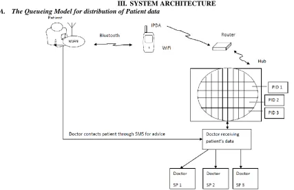
A. The Queueing Model for distribution of Patient data
ISSN: 2277-128X (Volume-7, Issue-6) PID 1 Patient ID 1: This can be from Pid 1 to Pid n.
SP 1 Specialist 1: This can also be form Sp 1 to Sp n.
Fig. 2: Block diagram of the queuing model
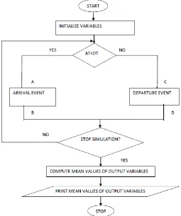
The M/M/1 queue consists of a server which provides service for the packets of data from the patients who arrive at the system and depart. It is a single-server queuing system with exponential interarrival times, exponential service times and first-in-first-out queue discipline. If a packet of data from a patient arrives when the server is busy, it joins the queue (the waiting line). There are two types of events: arrival events (A) and departure events (D). The following quantities are used in representing the model:
AT = arrival time DT = depature time
ISSN: 2277-128X (Volume-7, Issue-6)
Fig. 4: The first few events in simulation
In the first few events in simulation, the packets of data from the patient arrive the queueing model as the first arrival in time 0 and the interarrival time which is the time between the first arrival and the next arrival is denoted by T0 while the next arrival is denoted by T1. The first packets of data to arrive the queue is also the first to depart from the queue which is the first departure.
In the queueing model, vital signs are collected by the sensor on the patients’ body, sent through the Bluetooth (This data is simulated in the IPDA) to the IPDA which transmits this data by WiFi to the router which further transmits the data wirelessly to the hub which is in the server.
The hub acts as a data repository where these data are stored and sent to the doctor when there is an abnormal situation.
B. The Queueing Model
Queueing models can be represented using Kendall’s notation A/B/S/K/N/D
Where
A is the interarrival time distribution B is the service time distribution S is the number of servers K is the system capacity N is the calling population
D is the service discipline assumed
1) The Arrival Rate
The data arrive as packets of data from different patients wearing the sensors into the hub.
Let Ci be the interarrival time between the arrivals of the (i – 1)th and the ith patients, the mean(or expected) inter-arrival time is denoted by E(C) and is called β; = 1/E(C) the arrival frequency. The data is simulated in the IPDA and the interarrival time is 25 seconds and therefore β = 251 = 0.4.
2) Service Mechanism
This is specified by the number of servers (denoted by s) each server having its own queue or a common queue and the probability distribution of the patient’s service time.
Let Si be the service time of the ith patient, the mean service time of a customer is denoted by E(S) = 𝜇 = 1
𝐸 𝑆 the service rate of a server. The service time here is 10 seconds and therefore µ = 1
10 = 0.1.
3) Queue Discipline
Discipline of a queuing system means the rule that a server uses to choose the next patient from the queue (if any) when the server completes the service of the current patient.
The queue discipline for this system is
Single Server- (FIFO) First In First Out i.e. patients data are worked on according to when they came to the queue.
4) Measures of Performance for the Queuing System
Let
Di be the delay in queue of the ith patient 0
Interarrival time
T0
First arrival Next arrival
T1 Simulated time
Scheduled departure
ISSN: 2277-128X (Volume-7, Issue-6) Wi be the waiting time in the system of the ith patient
F(t) be the number of patients in queue at time t
G(t) be the number of patients in the system at time t = F(t) + No of patients served at t. Then the measures,
D = lim𝑛→∞ 𝐷𝑖 𝑖=𝑛 1=1
𝑛 and (1)
W =lim𝑛→∞ 𝑖=𝑛1=1𝑊𝑖
𝑛 (2)
are called the steady state average delay and the steady state average waiting time in the system. Also the measures,
F =lim𝑛→∞𝑇 1 𝐹 𝑡 . 𝑑𝑡0𝑇 and (3)
G = lim𝑛→∞𝑇 1 𝐺 𝑡 . 𝑑𝑡0𝑇 (4)
are called the steady state time average number in queue and the steady statetime average number in the system.
5) Single Channel Queue
[M/M/1] : {FCFS or FIFO} Queue System
6) Arrival Time Distribution
This model assumes that the number of arrivals occurring within a given interval of time t, follows a poisson distribution with parameter 𝛽 𝑡. This parameter 𝛽 𝑡 is the average number of arrivals in time t which is also the variance of the distribution. If n denotes the number of arrivals within a time interval t, then the probability function p(n) is given by P(n) = (𝛽 )
𝑛
𝑛! 𝑒
−𝑥 n = 0,1,2…. (5)
The arrival process is called poisson input
The probability of no(zero) arrival in the interval [0,t] is, Pr (zero arrival in [0,t]) = 𝑒−𝛽𝑡 = p(0)
Also
P(zero arrival in [0,t]) = P(next arrival occurs after t) = P(time between two successive arrivals exceeds t)
Therefore the probability density function of the inter- arrival times is given by, 𝑒−𝛽𝑡for t > 0
This is called the negative exponential distribution with parameter 𝛽 or simply exponential distribution. The mean inter-arrival time and standard deviation of this distribution are both 1/(𝛽) where, (𝛽)is the arrival time.
7) Performance Measures
The average number of units in the system G can be found from G = sum of [n*Pn] for n = 1 to ∞
G = 𝛽 𝜇 −𝛽 =
𝑃
1−𝑃 where P = 𝛽
𝜇 (6)
The average number in the queue is
F = (G – (1 – P0) (7)
Sum of [(n-1)*Pn] for n = 1 to ∞
F = 𝛽2 𝜇 (𝜇 −𝛽 ) =
𝑃2
(1−𝑃) (8)
The average waiting time in the system (time in the system) can be obtained from
W = 𝐺 𝛽 =
1
𝜇 −𝛽 and (9)
D = W -1 𝜇=
𝛽
𝜇 .(𝜇 −𝛽 ). (10)
The traffic intensity P (sometimes called occupancy) is defined as the average arrival rate (lambda) divided by the average service rate (mu). P is the probability that the server is busy.
P = 𝛽𝜇 (11)
The mean number of customers in the system (N) can be found using the following equation:
(12) You can see from the above equation that as p approaches 1 number of customers would become very large. This can be easily justified intuitively. p will approach 1 when the average arrival rate starts approaching the average service rate. In this situation, the server would always be busy hence leading to a queue build up (large N).
Lastly we obtain the total waiting time (including the service time): T = 1
ISSN: 2277-128X (Volume-7, Issue-6)
IV. RESULTS
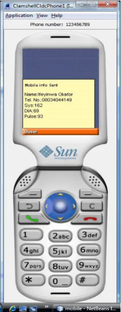
A program was written in java to simulate the remote patient monitoring system. A simulated mobile phone called the Intelligent Personal Digital Assistant (IPDA) was used for the simulation. It generates the patients’ vital signs which are sent to the queueing model. These readings are generated every twenty five seconds. The queueing model stores these records according to when they arrive. A graph can also be plotted using the readings for each patient so that the doctor can view each patients’ readings at a glance and proffer his solution.The results of these simulations are shown in the figures below:
Fig. 5: The IPDA Fig. 6: The simulated reading for a patient
ISSN: 2277-128X (Volume-7, Issue-6)
Fig. 8: The Mobile Queue
Fig. 9: The graph for a patient showing the readings of the vital signs
V. CONCLUSION
ISSN: 2277-128X (Volume-7, Issue-6) The queueing model was adapted and incorporated into the work to store these readings of the vital signs of patients. The queueing model called the mobile queue in this work gives a summary of the total number of readings generated for each patient, the time of arrival, the number of channels, the service time, the service rate, the mean patient arriving the system and the traffic intensity.
It is shown also that the queueing model enhances the remote patient medical monitoring system by giving the doctor the detailed readings of each patient’s medical records at a glance. This aids optimum performance of the system and saves lives.
REFERENCES
[1] K. E. Agner (2013) plus.maths.org".[Online] Availablehttp://www.pass.maths.org.uk.
[2] S. R.Asmussen, O. J. Boxma, "Editorial introduction". Queueing Systems. vol. 63: 1. doi:10.1007/s11134-009-9151-8 2009.
[3] J. A. Buzacott, J. G.Shanthikumar,Stochastic models of manufacturing systems, Prentice Hall, Englewood Cliffs,
1993.
[4] A. K. Erlang, (1909). "The theory of probabilities and telephone conversations" (PDF). NytTidsskrift for Matematik B. vol. 20 pp. 33–39. Archived from the original (PDF) on 2011-10-01.
[5] G. Feck, E. L. Blair, C. E. Lawrence , “A systems model for burn care”,Med Carevol. 18, pp. 211–218, 1980.
[6] P. R. Harper, A. K. Shahani, “Modelling for the planning and management of bed capacities in hospitals”,
JOper Res Soc vol. 53, pp. 11–18, 2002.
[7] J. CHershey, E. N. Weiss, M. A. Cohen,“A stochastic service network model with application to hospital facilities”, Oper Resvol. 29, pp. 1–22, 1981.
[8] D. G. Kendall, "Stochastic Processes Occurring in the Theory of Queues and their Analysis by the Method of the Imbedded Markov Chain". The Annals of Mathematical Statistics. vol. 24, pp. 338. doi:10.1214/aoms/1177728975. JSTOR 2236285, 1953.
[9] D.G.Kendall, “Stochastic processes occurring in the theory of queues and their analysis by the method of the imbedded Markov chain”, Ann. Math. Stat. 1953.
[10] J. F. C. Kingman, "The first Erlang century—and the next". Queueing Systems. vol. 63, pp. 3–4. doi:10.1007/s11134-009-9147-4, 2009.
[11] J. F. C. Kingman, Atiyah, "The single server queue in heavy traffic".Mathematical Proceedings of the Cambridge Philosophical Society, vol.57pp. 902. doi:10.1017/S0305004100036094. JSTOR 2984229, 1961.
[12] W. D. Lawrence,A.F. A.Virgilio, A. M. Daniel."Performance by Design: Computer Capacity Planning by Example".
[13] A.A. Markov,“Extension of the law of large numbers to dependent quantities”, IzvestiiaFiz.-Matem. Obsch. Kazan Univ., (2nd Ser.), vol. 15 pp. 135–156, 1906.
[14] L. Mayhew, S. David, Using queuing theory to analyse completion times in accident and emergency departments in the light of the Government 4-hour target. Cass Business School. ISBN 978-1-905752-06-5. 2006.
[15] S.Park, S.Jayaraman, “Enhancing the Quality of Life Through Wearable Technology,” in IEEE Engineering in Medicine and Biology Magazine, vol. 22, pp. 41–48, 2003.
[16] F. Pollaczek, ProblèmesStochastiquesposés par le phénomène de formation d'une queue [17] F. Pollaczek, UebereineAufgabe der Wahrscheinlichkeitstheorie, Math. Z, 1930
[18] K. Schlechter, "Hershey Medical Center to open redesigned emergency room". The Patriot-News, 2009.
[19] V. Sundarapandian, V. Queueing Theory. Probability, Statistics and Queueing Theory. PHI Learning. ISBN 8120338448, 2009.
[20] H. C. Tijms, Algorithmic Analysis of Queues, Chapter 9 in A First Course in Stochastic Models, Wiley, Chichester, 2003.
[21] J. Walrand,An introduction to queueing networks, Prentice Hall, Englewood Cliffs, 1988.
[22] E. N. Weiss J. O.McClain“Administrative days in acute care facilities: A queueing-analytic approach”,Oper Res
vol. 35, pp.35–44, 1987.