ISSN 2307-7743 http://scienceasia.asia
MODELLING THE IMPACT OF BEMISIA TABACI IN DYNAMICS OF TOMATO YELLOW LEAF CURL VIRUS
CHRISTOPHER NGALYA∗, DMITRY KUZNETSOV
Abstract. Mathematical model has been developed and analysed for the interaction
be-tween tomato yellow leaf curl virus (TYLCV) and tomato plants under the influence of Bemisia tabaci. Positivity and boundedness of the solution has been checked to ensure our
model being well posed and then we computed the basic reproductive numberR0 using the
next generation matrix method. Also, both local and global stability analysis at the disease
free equilibrium points of the model has been done. By constructing suitable Lyapunov functional and using LaSalle’s invariance principle, global stability of endemic disease
equi-librium was obtained. The results show that the disease free equiequi-librium point (DFE) will be both locally and globally asymptotically stable if R0 < 1 but unstable if R0 > 1 and
the endemic equilibrium point (EE) will be globally asymptotically stable if R0 >1 and
unstable ifR0<1. Finally some numerical simulations were done to validate our theoretical
outcomes, and the epidemiological implications of the key outcomes were briefly discussed in the last section.
1. Introduction
Tomato yellow leaf curl virus (TYLCV) is the name given to complex virus species that causes disease known as tomato yellow leaf curl disease (TYLCD). Tomato yellow leaf curl virus (TYLCV) is a major threat to the tomato crop in many tropical and sub-tropical regions[12]. TYLCV is transmitted by the insect vector Bemisia tabaci (whitefly). The virus accounts for huge losses in quantity and quality of tomatoes if unchecked. Incidences as high as 100% with undesirable consequences of crop failure have been recorded[15, 5]. The virus was detected first in Israel around 1930, and currently it affects about 30 countries around the world that grow tomatoes. Symptoms of TYLCV that exhibited by tomato plants is reduction in leaf size, leaf curling upward, severe stunting and distortion associated with interveinal chlorosis, observed mainly on the upper portion of plants[16, 13].The disease is among the major virus diseases that causes low yields of tomatoes in Tanzania, especially, in farmer’s fields. Disease occurrence of about 100% had been reported in some regions in Tanzania mainland[9, 14].
Key words and phrases. TYLCD; TYLCV; Bemisia tabaci; Basic reproductive number, Stability analysis.
c
2017 Science Asia
2. Formulation of the TYLCD model
Plant population has been divided into three categories in SEI type structure, reflecting the disease status: susceptible (healthy), exposed (latent infection) and infectious. Similarly we have defined categories for the vector population in SI type structure as susceptible (non infectious) and infective which links the epidemiology of disease with the population dynamics of the vector. In SEI, the total tomato population NT was subdivided into three
sub-populations; tomato plants that are susceptible to infection with TYCLV ST, those
exposed to TYCLVET and infectious tomato plantsIT. That isNT =ST+ET+IT. The total
whitefly vector population NV is sub-divided into two sub-populations; susceptible whitefly
vector population SV and infectious whitefly vector population IV. That is NV =SV +IV.
The transmission dynamics of TYLCV is summarised in the compartmental diagram in Figure 2.1.
Figure 1. Compartmental diagram for the transmission dynamics of TYLCV
The model assumes that a year-round vegetable production system is used. Replanting took place at a rate which exactly balanced those plants removed. This means that we maintain a host population at a constant size by balancing the birth and death (or replanting and mortality) rates. Farmers plant only healthy varieties of tomato in a garden of carrying capacityK, no death of tomato plants before harvesting and the whitefly vectors are assumed to remain infectious once they acquire the virus. The variables and the parameters are summarised in Tables 2.1 and 2.2.
Table 1. Model Variables
Variable Description
ST Susceptible tomato plants
ET Exposed tomato plants
IT Infectious plants
NT Total plant population
SV Susceptible whitefly
IV Infectious whitefly
NV Total whitefly population
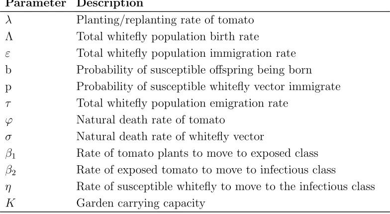
Table 2: Model Parameters
Parameter Description
λ Planting/replanting rate of tomato
Λ Total whitefly population birth rate
ε Total whitefly population immigration rate b Probability of susceptible offspring being born p Probability of susceptible whitefly vector immigrate
τ Total whitefly population emigration rate
ϕ Natural death rate of tomato
σ Natural death rate of whitefly vector
β1 Rate of tomato plants to move to exposed class
β2 Rate of exposed tomato to move to infectious class
η Rate of susceptible whitefly to move to the infectious class
K Garden carrying capacity
From the compartmental diagram in Figure 2.1 and basing on assumptions and descrip-tions made we derive the following equadescrip-tions:
(1)
dST
dt =λ(1− NT
K )−
β1IVST
NT
−σST,
dET
dt =
β1IVST
NT
−β2ET −σET,
dIT
dt =β2ET −σIT. Vector equations
(2)
dSV
dt = Λ +pτ − ηITSV
NV
−ϕSV −εSV,
dIV
dt = (1−b)Λ + (1−p)τ + ηITSV
NV
−ϕIV −εIV.
3. Basic properties of the model
3.1. Positivity. In order the TYLCD model to be meaningful epidemiologically, we must show that all state variables are non-negative for all times t ≥ 0. We find solution of each equation in systems (1) and (2) in their patches for testing positivity.
Lemma 3.1. Let the initial data be {(ST(0), ET(0), IT(0), SV(0), IV(0)) > 0} ∈ Ω; then
solution set {ST(t), ET(t), IT(t), SV(t), IV(t)} of the model system is positive ∀t >0.
Proof. From the first equation of the tomato plant population of the model system (1),
dST
dt =λ(1− NT
K )−
β1IVST
NT
−σST.
(3) dST
dt ≥ −( β1IV
NT
−σ)ST(t).
By separating variables and integrating both sides of the equation (3) above we obtain,
ST(t)≥ST(0)e
−(β1IV
NT −σ)t≥0. ThereforeST(t)>0.
Following similar procedure we can compute all variables ET(t), IT(t), SV(t) and IV(t) and
establish thatET(t), IT(t), SV(t) andIV(t)>0.
Therefore the solution set{ST(t), ET(t), IT(t), SV(t), IV(t)}of the model is positive ∀t >0.
3.2. Invariant region. Since the system is modelling tomato plants and whitefly vector populations, we assumed that the state variables and parameters of the model are completely non-negative t ≥ 0. The TYLCD transmission model has two compartments where each population is treated separately.
Lemma 3.2. All forward solutions of the of the TYLCD model in R5
+ enter the invariant region Ω = ΩT+ ΩV where ΩT ={(ST, ET, IT)∈: (ST+ET +IT =NT)}, ΩV ={(SV, IV)∈:
(SV +IV =NV)}, and Ω is the invariant region of the whole system.
of equations in system (1) yield NT
dt = λ(1−
NT
K )−σNT. By separating variables in this
equation, applying an integrating factor technique we compute the differential equation and obtain,
NT =
λ+Kλ K +Ce
−(Kλ+σ)t.
NT =
λ+Kλ
K + (NT(0)−
λ+Kλ K )e
−(Kλ+σ)t.
when t−→ ∞NT(t)−→ λ+KKλ, fort= 0, NT(t) =NT(0) which implies thatNT(t)≥0.
Let NT be the total population of the whitefly vector, then NV = ST +IV. Addition of
equations in system (2) yield NV
dt = 2(bΛ +pτ−1)−(ϕ+ε). By separating variables in this
equation, applying an integrating factor technique we compute the differential equation and obtain,
NV =
2(bΛ +pτ −1)
ϕ+ε +Ce
−(ϕ+ε)t
.
NV =
2(bΛ +pτ −1)
ϕ+ε + (NV(0)−
2(bΛ +pτ −1)
ϕ+ε )e
−(ϕ+ε)t, where (ϕ+ε)6= 0.
when t −→ ∞ NV(t) −→
2(bΛ+pτ−1)
ϕ+ε , for t = 0, NV(t) = NV(0) which implies that
NV(t)≥0.
Therefore since NT(t) > 0 and NV(t) > 0 , hence the set {(ST, ET, IT) ∈ R3+; ((SV, IV) ∈
R2
+)} is a positive invariant set in Ω.
4. Model analysis
4.1. Disease free equilibrium point D0. At disease free,dET
dt = dIT
dt = dIV
dt = 0, dST
dt =λ(1−
NT K )−
β1IVST
NT −σST, λ(1− NT
K )− β1IVST
NT −σST = 0.
But since at disease free, IV = 0, ST = NT therefore λ(1− STK)−σST = 0. Making ST the
subject, we obtain ST = σKλK+λ. Considering following equations,
dSV
dt = Λ +pτ −
ηITSV NV −
ϕSV −εSV,
dIV
dt = (1−b)Λ + (1−p)τ +
ηITSV
NV −ϕIV −εIV.
(4) Λ +pτ − ηITSV
NV
−ϕSV −εSV = 0,
(5) (1−b)Λ + (1−p)τ + ηITSV
NV
−ϕIV −εIV = 0.
Addition of these equations (4) and (5), resultsbΛ +pτ −ϕSV −εSV + (1−b)Λ + (1−p)τ−
ϕIV −εIV = 0. But IV = 0.
bΛ +pτ −ϕSV −εSV + (1−b)Λ + (1−p)τ = 0, SV = bΛ+ϕ+pτε .
Therefore the D0 of the model system is given by ( λK σK+λ,0,0,
4.2. Endemic equilibrium point D∗. In the presence of TYLCD, ET 6= 0, IT 6= 0, IV 6=
0 our model has an equilibrium point called endemic equilibrium point denoted D∗ = (ST∗, ET∗, IT∗, SV∗, IV∗) 6= 0. D∗ is the steady state solution where TYLCD persist in the pop-ulation of tomato plants. For the existence of D∗, the elements must satisfy; ST∗ >0, ET∗ >
0, IT∗ >0, SV∗ >0, IV∗ >0.We find the endemic equilibrium point by setting the right side of the model system equations (1) and (2) equal to zero. Thus;
IT∗ = β2σ(bΛ+pτ)−(ϕ+ε)
β2ηλ(1−
N∗ T K )−(β2σ)
,
ST∗ = λσ(1− NT∗ K )−
I∗
T
β2(β2+σ), ET∗ = σIβ∗T
2 , ST∗ = (bΛ+pτ)NV∗
ηI∗
T+(ϕ+ε)NV∗,
IV∗ = NV∗(I
∗
T+(ϕ+ε))((1−b)Λ+(1−p)τ)+IT N V(bΛ+pτ)
(ϕ+ε)(ηIT∗+(ϕ+ε)NV∗) .
For a positive endemic equilibrium point, the conditions λσ(1− NT∗ K )>
IT∗
β2(β2+σ), β2σ(bΛ + pτ)>(ϕ+ε) and β2ηλ(1−
NT∗
K )>(β2+σ) must hold.
4.3. The basic reproduction number R0. The basic reproduction number (R0) is the expected number of secondary cases produced by a single infection into a completely sus-ceptible population[1]. [3] defined R0 as a spectral radius (ρ(F V−1)) of the next generation matrix. This is a parameter which usually tells if the epidemiologic might persist or die out within a purely susceptible population. The epidemiological criterion ofR0 is that ifRo >1 then the disease free equilibrium point is unstable and can invade the population and persist for long time [17]. There are several methods for calculating R0 but in this study the next generation operator method as proposed by [17] is used.
The disease transmission model comprised of the system of equations Xj∗ =Fj(x)−Vj(x),
where Fj(x) is for new infection and Vj(x) is for remaining transfer terms. To obtain the
matrix F and V (Jacobian matrices), we then find derivatives of vectors Fj(x) and Vj(x)
respectively.
From the model equation,
Fj(x0) =
β1IVST
NT
0
(1−b)Λ + (1−p)τ +ηITNVSV
.
The Jacobian matrix at D0 is
F =
0 0 β1
0 0 0
0 η 0
From the model equation,
Vj(x)=
β2ET +σET
σIT −β2ET
ϕIV +εIV
.
The Jacobian matrix at D0 is
V =
β2+σ 0 0
−β2 σ 0
0 0 ϕ+ε
, and V
−1=
1
β2+σ 0 0
β2
β2+σ
1
σ 0
0 0 ϕ1+ε
.
Multiplying F and V−1 yields a next generation matrixF V−1 as shown below,
F V−1 =
0 0 β2
ϕ+ε
0 0 0
β2η
β2+σ
η
σ 0
.
Computing the maximum eigen value of the next generation matrix we getR0 =
q
β1β2η
(ϕ+ε)(β2+σ). R0 is a threshold parameter that indicates the average number of infected vectors and in-fected hosts caused by a cross-infection of one tomato plant host or one whitefly vector when the other population consist of only susceptible [10]. The square root arises from the fact that dual generations are necessary for transmission of TYLCD to take place, i.e. From an infectious tomato plant to a susceptible whitefly vector and then from an infectious whitefly vector to susceptible tomato plant(host) [10].
4.4. Stability analysis.
4.4.1. Local stability of the disease free equilibrium point. We examine the stability of the disease free equilibrium point D0 = ( λK
σK+λ,0,0, bΛ+pτ
ϕ+ε ,0) by employing the method used by
Kinene et al. (2015).
Lemma 4.1. The disease free equilibrium D0 is locally asymptotically stable if R0 <1 but unstable if R0 >1, where R0 is the basic reproduction number.
Proof. We linearize the model system (1) and (2) by computing its Jacobian matrix JD0.
The Jacobian matrix is computed at disease free equilibrium point by differentiating each equation in the system with respect to the state variables ST, ET, IT, SV,and IV. Therefore
the Jacobian matrix is
(6) JD0 =
−β1IV
NT −σ 0 0 0 −β1
0 −β2−σ 0 0 β1
0 β2 −σ 0 0
0 0 −η −(Sη
V +ϕ+ε) 0
0 0 η 0 −ϕ−ε
It is clear from equation (6) that the first and second eigen values are λ1 = −σ and
λ2 =−(ηb(Λ+ϕ+pτε) +ϕ+ε). This can be reduced to a (3×3) matrix
(7) JD0 =
−β2−σ 0 β1
β2 −σ 0
0 η −ϕ−ε
.
Its characteristics polynomial is
(ε+µ+ 2σ+β2)λ2+ (σ2+ (2µ+ 2ε+β2)σ+β2(ε+µ))λ+ (ε+µ)σ2+ (ε+µ)β2σ−β1β2η+ (ε+µ+ 2σ+β2)λ2+ (σ2+ (2µ+ 2ε+β2)σ+β2(ε+µ))λ+ (ε+µ)σ2+ (ε+µ)β2σ−β1β2η.
a1 =ε+µ+2σ+β2, a2 = (σ2+(2µ+2ε+β2)σ+β2(ε+µ)), a3 = (ε+µ)σ2+(ε+µ)β2σ−β1β2η. Consider (ε+µ+ 2σ+β2)>0. Since all model parameters are positive, it is obvious that
a1 is positive (a1 >0). Consider (σ2+ (2µ+ 2ε+β
2)σ+β2(ε+µ))>0. From the point that all model parameters are positive, it is obvious that a2 is positive (a2 >0).
In order that a3 being positive, (ε+µ)σ2+ (ε+µ)β2σ−β1β2η >0. (ε+µ)σ2+ (ε+µ)β
2σ > β1β2η, 1> (ε+µ)σβ21+(β2εη+µ)β
2σ, 1> R2
0
σ .
a1a2−a3 = (ε+µ+2σ+β2)∗(σ2+(2µ+2ε+β2)σ+β2(ε+µ))−((ε+µ)σ2+(ε+µ)β2σ−β1β2η). After simplification yields a1a2−a3 >0.
By Routh-Hurwitz criteria all eigenvalues have negative real parts if R0 < 1 thus making the disease free equilibrium locally asymptotically stable.
4.4.2. Global stability of the disease free equilibrium point. We examine global stability of the disease free equilibrium using the theorem proposed by [2] similar as in [10]. Thus we rewrite our model and mention two conditions, if satisfied will guarantee global asymptotic stability of the disease free equilibrium.
(8) F(X, Z) =
dX
dt =F(X, Z), dZ
dt =G(X, Z), G(X, Z) = 0,
where X = (ST, SV) ∈ R2 denote susceptible populations and Z = (ET, IT, IV) ∈ R3
denote infected populations. D0 = (X∗,0) represent the disease free equilibrium of this system. The conditions (i) and (ii) below guarantee global asymptotic stability:
(i): for dX
dt =F(X,0), X
∗ is global asymptotically stable.
(ii): G(X, Z) = DZG(X∗, Z)Z −Gˆ(X, Z), Gˆ(X, Z)≥0 for, (X, Z)∈Ω,
where DZG(X∗, Z) is Metzler Matrix (the off diagonal elements are non negative) and also
the Jacobian ofG(X, Z) taken in (ET, IT, IV) and evaluated at (X∗,0) = (σKλK+λ,bΛ+ϕ+pτε ,0,0,0).
Lemma 4.2. The equilibrium point D0 = (X∗,0)of the system (8) is globally
asymptoti-cally stable if R0 ≤1 and the conditions (i) and (ii) are satisfied.
Proof. We now start our proof by describing new variables and breaking the system into subsystems. X = (ST, SV) and Z = (ET, IT, IV). From equation (8) we have two vector
valued functions G(X.Z) and F(X,Z) given by:
F(X, Z) =
λ(1− NT K )−
β1IVST
NT −σST,
bΛ +pτ − ηITNVSV −ϕSV −εSV,
G(X, Z) =
β1IVST
NT −β2ET −σET,
β2ET −σIT,
(1−b)Λ + (1−p)τ+ ηITNVSV −ϕIV −εIV.
For condition (i) we considering the reduced system dX
dt =F(X,0).
(9) F(X, Z) =
dST
dt =λ(1−
NT K )−
β1IVST
NT −σST,
dSV
dt =bΛ +pτ −
ηITSV
NV −ϕSV −εSV.
X∗ = (σKλK+λ,bΛ+ϕ+pτε ) is globally asymptotically stable equilibrium. To prove this, we find
the solution of dX
dt = F(X,0). When we find solution of the first equation from (9) yields ST = σKλK+λ + (ST(0)− σKλK+λ)e−(
σK+λ
λK )t that approaches λK
σK+λ if t −→ ∞. Similarly solving
the second equation of (9) yields SV = bΛ+ϕ+pτε + (SV(0) − bΛ+ϕ+pτε ) e−( bΛ+pτ
ϕ+ε )t that
approach-es bΛ+ϕ+pτε ift −→ ∞regardless of the initial condition. Thus, is globally asymptotically stable.
Meanwhile for condition (ii) we compute G(X, Z) =DZG(X∗, Z)Z−Gˆ(X, Z), and then
prove that ˆG(X, Z)≥0, f or (X, Z)∈Ω.
G(X, Z) =
β1IVST
NT −β2ET −σET
β2ET −σIT
(1−b)Λ + (1−p)τ +ηITNVSV −ϕIV −εIV
.
At disease free equilibrium point,
DZG(X∗,0)=
−(β1+σ) 0 β1
β2 −σ 0
0 η −(ϕ+ε)
, DZG(X
∗,0)Z=
(β1+σ)ET +β1IV
β2ET −σIT
ηIT −(ϕ+ε)IV
.
ˆ
G(X, Z) =
−(β1+σ)ET +β1IV
β2ET −σIT
ηIT −(ϕ+ε)IV −
β1IVST
NT −β2ET −σET
β2ET −σIT
(1−b)Λ + (1−p)τ +ηITSVNV −ϕIV −εIV
.
ˆ
G(X, Z) =
β1IV(1− NTST)
0
ηIT −((1−b)Λ + (1−p)τ +ηITNVSV)
.
Since (1−ST
NT)≥0 thenβ1IV(1− ST
NT)≥0,meanwhile forηIT ≥((1−b)Λ+(1−p)τ+ ηITSV
NV )
thenηIT−((1−b)Λ + (1−p)τ+ηITNVSV)≥0.Therefore ˆG(X, Z)≥0 and hence this completes
the proof of lemma 4.2.
4.4.3. Global stability of endemic equilibrium point. Global stability of the endemic equi-librium point D∗ is analyzed by constructing a suitable Lyapunov function. We prove for global stability of endemic equilibrium point following the approach used by [8] and other several epidemiological models. We consider the Lyapunov function of the form
L=P
Pi(Ri−Ri∗ln(Ri)).
So we define the Lyapunov function as L(ST, IT, SV, IV) = P1(ST −ST∗ ln(ST)) +P2(ET −
ET∗ ln(ET)) +P3(IT −IT∗ln(IT)) +P4(SV −SV∗ ln(SV)) +P5(IV −IV∗ ln(IV)).
We can now verify the condition dL
dt ≤0. Proof. The time derivative of L is dL
dt =P1(1−
ST∗ ST)
dST
dt +P2(1−
E∗T ET)
dET
dt +P3(1−
IT∗ IT)
dIT
dt + P4(1−
S∗
V SV)
dSV
dt +P5(1−
I∗
V IV)
dIV
dt
= P1(1−
S∗
T
ST)(λ(1− NT
K )− β1IVST
NT −σST) +P2(1− E∗
T ET)(
β1IVST
NT −β2ET −σET) +P3(1− IT∗
IT)(β2ET −σIT) +P4(1− SV∗
SV)(bΛ +pτ − ηITSV
NV −ϕSV −εSV) +P5(1− IV∗
IV)((1−b)Λ + (1−
p)τ+ ηITNSV
V −ϕIV −εIV).
At an endemic equilibrium pointD∗ we haveλ(1−NT K ) = (
β1IV
NT +σ)S
∗
T, β1IVST
NT = (β2+σ)E
∗
T,
β2ET. =σIT∗,bΛ +pτ = ( ηITSV
NV +ϕ+ε)S
∗
V and ((1−b)Λ + (1−p)τ+ ηITSV
NV = (ϕ+ε)I
∗
V.
=P1(1−
ST∗ ST)((
β1IV
NT +σ)S
∗
T −( β1IV
NT +σ)ST) +P2(1− ET∗
ET)((β2+σ)E
∗
T −(β2+σ)ET) +P3(1−
IT∗ IT)(σI
∗
T−σIT)+P4(1−
S∗V SV)(
ηIT
NV +ϕ+ε)S
∗
V−( ηIT
NV +ϕ+ε)SV+P5(1− IV∗
IV)((ϕ+ε)I
∗
V−(ϕ+ε)IV).
=−P1(1−
S∗
T ST)
2σ)S
T−P1(βNT1IV(1−
S∗
T ST)(1−
S∗
TI
∗
V
STIV)−P2(1− E∗
T ET)
2(β
2+σ)ET−P3(1−
I∗
T IT)
2σI
T−
P4(1−
SV∗ SV)
2(ϕ+ε)S
V −P4ηITNVSV(1−
SV∗ SV)(1−
IT∗SV∗
ITSV)−P5(1− IV∗ IV)
2I
V(ϕ+ε).
=−P1(1−
S∗T ST)
2σ)S
T −P2(1−
E∗T ET)
2(β
2+σ)ET −P3(1−
IT∗ IT)
2σI
T −P4(1−
SV∗ SV)
2(ϕ+ε)S
V −
P5(1−
I∗
V IV)
2I
V(ϕ+ε) +P(ST, ET, IT, SV, IV),
where P(ST, ET, IT, SV, IV) = (−P1(βNT1IV(1−
S∗
T ST)(1−
S∗
TIV∗ STIV)−P4
ηITSV NV (1−
S∗
V SV)(1−
I∗
TS∗V
ITSV))<0.
The function P(ST, ET, IT, SV, IV) is non-positive by considering the method used by [8].
Thus P(ST, ET, IT, SV, IV) < 0 for all ST, ET, IT, SV, IV >0. Hence,
dL
dt ≤ 0 and dL
dt = 0
invariant set such that dL
dt = 0 is the singleton{D
∗}which is our endemic equilibrium point.
By LaSalle’s invariant principle in [11] we conclude thatD∗ is globally asymptotically stable if R0 >1 and unstable if R0 <1. So, we establish the following lemma.
Lemma 4.3. The endemic equilibrium pointD∗ of the model systems (1) and (2) is globally asymptotically stable if R0 >1 and unstable otherwise.
5. Numerical Simulation and Discussion
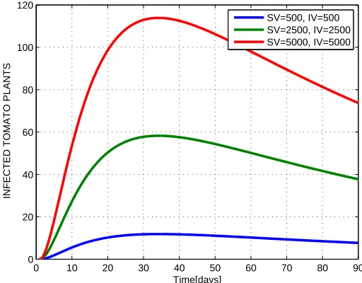
The main intention of this paper is to assess the impact of number of bemisia tabaci interacting with tomato plants in transmission of TYLV. In order to support the analytical results, numerical simulations were performed using different values for the initial number of vectors but constant number of host population (tomato plants) and using numerical value of parameter taken from literature while some were estimated. Fixed variables used are
ST=2000,ET=IT=0, while other variable were varying (SV=IV=500, 2500 and 5000). The
final time is tf=90 days, and the rest parameters values are shown in the Table 5.1.
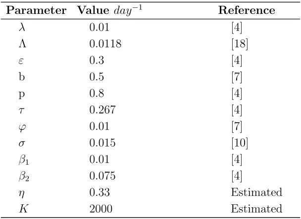
Table 3: Parameter values for the model
Parameter Value day−1 Reference
λ 0.01 [4]
Λ 0.0118 [18]
ε 0.3 [4]
b 0.5 [7]
p 0.8 [4]
τ 0.267 [4]
ϕ 0.01 [7]
σ 0.015 [10]
β1 0.01 [4]
β2 0.075 [4]
η 0.33 Estimated
K 2000 Estimated
0 10 20 30 40 50 60 70 80 90 600
800 1000 1200 1400 1600 1800 2000
Time[days]
SUSCEPTIBLE TOMATO PLANTS
SV=500, IV=500 SV=2500, IV=2500 SV=5000, IV=5000
Figure 2. Graph of susceptible tomato plants vs. time for the first 90 days of growth
0 10 20 30 40 50 60 70 80 90
0 20 40 60 80 100 120
Time
EXPOSED TOMATO PLANTS
SV=500, IV=500 SV=2500, IV=2500 SV=5000, IV=5000
0 10 20 30 40 50 60 70 80 90 0
20 40 60 80 100 120
Time[days]
INFECTED TOMATO PLANTS
SV=500, IV=500 SV=2500, IV=2500 SV=5000, IV=5000
Figure 4. Graph of infected tomato plants vs. time for the first 90 days of growth
Numerical simulation results in Figure 5.1 shows significant decrease in the number of sus-ceptible plants due to increase of number of vectors in the field. Figure 5.2 shows an increase in the number of exposed plants due to increase of number of vectors in the field and Figure 5.3 shows also the increase in the number of infected plants due to increase of number of vectors. This implies that the increase of number of vectors around the field lead to decrease of amount of tomato yield in that field due to TYLCV.
6. Conclusion
References
[1] R. Anderson and R. May, Infectious diseases of humans. oxford university press,
oxford., 757 p, (1991).
[2] C. Castillo-Chavez, S. Blower, P. Driessche, D. Kirschner, and A.-A.
Yakubu, Mathematical approaches for emerging and reemerging infectious diseases:
models, methods, and theory, Springer, 2002.
[3] O. Diekmann, J. Heesterbeek, and J. Metz, On the definition and the
computa-tion of the basic reproduccomputa-tion ratio r0 in models for infectious, Phil. Trans. R. Soc. B, 9 (1990), pp. 356–382.
[4] J. Holt, J. Colvin, and V. Muniyappa, Identifying control strategies for tomato
leaf curl virus disease using an epidemiological model, Journal of Applied Ecology, 36 (1999), pp. 625–633.
[5] N. Ioannou,Yellow leaf curl and other virus diseases of tomato in cyprus, Plant
pathol-ogy, 34 (1985), pp. 428–434.
[6] M. Jeger, J. Holt, F. Van Den Bosch, and L. Madden,Epidemiology of insect-transmitted plant viruses: modelling disease dynamics and control interventions, Physi-ological Entomology, 29 (2004), pp. 291–304.
[7] M. Jeger, F. Van Den Bosch, L. Madden, and J. Holt, A model for
analysing plant-virus transmission characteristics and epidemic development, Mathe-matical Medicine and Biology: A Journal of the IMA, 15 (1998), pp. 1–18.
[8] J. Kahuru, L. Luboobi, and Y. Nkansah-Gyekye, Stability analysis of the
dy-namics of tungiasis transmission in endemic areas, Asian Journal of Mathematics and Applications, 2017 (2017).
[9] B. D. Kashina, R. B. Mabagala, and A. A. Mpunami,Biomolecular relationships among isolates of tomato yellow leaf curl tanzania virus, Phytoparasitica, 31 (2003), pp. 188–199.
[10] T. Kinene, L. S. Luboobi, B. Nannyonga, and G. G. Mwanga,A mathematical
model for the dynamics and cost effectiveness of the current controls of cassava brown streak disease in uganda, Journal of Mathematical and Computational Science, 5 (2015), p. 567.
[11] J. P. La Salle,The stability of dynamical systems, SIAM, 1976.
[12] K. Makkouk, H. Laterrot, et al.,Epidemiology and control of tomato yellow leaf
curl virus., Epidemiology and control of tomato yellow leaf curl virus., (1983), pp. 315– 321.
[13] P. V. Mart´ınez-Culebras, I. Font, and C. Jord´a, A rapid pcr method to
dis-criminate between tomato yellow leaf curl virus isolates, Annals of applied biology, 139 (2001), pp. 251–257.
G. Marchoux, R. Opena, et al.,Tomato viruses in tanzania: identification,
distri-bution and disease incidence., Journal of the Southern African Society for Horticultural Sciences, 6 (1996), pp. 41–44.
[15] B. Pic´o, M. J. D´ıez, and F. Nuez,Viral diseases causing the greatest economic losses
to the tomato crop. ii. the tomato yellow leaf curl virusa review, Scientia Horticulturae, 67 (1996), pp. 151–196.
[16] R. Salati, M. K. Nahkla, M. R. Rojas, P. Guzman, J. Jaquez, D. P.
Maxwell, and R. L. Gilbertson, Tomato yellow leaf curl virus in the
domini-can republic: characterization of an infectious clone, virus monitoring in whiteflies, and identification of reservoir hosts, Phytopathology, 92 (2002), pp. 487–496.
[17] P. Van den Driessche and J. Watmough,Reproduction numbers and sub-threshold
endemic equilibria for compartmental models of disease transmission, Mathematical bio-sciences, 180 (2002), pp. 29–48.
[18] X.-S. Zhang, J. Holt, and J. Colvin, A general model of plant-virus disease
infec-tion incorporating vector aggregainfec-tion, Plant Pathology, 49 (2000), pp. 435–444.
The Nelson Mandela African Institution of Science and Technology, P.O Box 447, Arusha-Tanzania