A MODEL OF AGE–STRUCTURED POPULATION
UNDER STOCHASTIC PERTURBATION OF DEATH
AND BIRTH RATES
1Maxim A. Alshanskiy
Ural Federal University, Ekaterinburg, Russia
Abstract: Under consideration is construction of a model of age-structured population reflecting random oscillations of the death and birth rate functions. We arrive at an Itˆo-type difference equation in a Hilbert space of functions which can not be transformed into a proper Itˆo equation via passing to the limit procedure due to the properties of the operator coefficients. We suggest overcoming the obstacle by building the model in a space of Hilbert space valued generalized random variables where it has the form of an operator-differential equation with multiplicative noise. The result on existence and uniqueness of the solution to the obtained equation is stated.
Key words: Brownian sheet, Cylindrical Wiener process, Gaussian white noise, Stochastic differential equation, Age-structured population model.
Introduction
A well known model of an age-structured population dynamics is the famous McKendrick–von Foerster equation
∂u(x, t)
∂t +
∂u(x, t)
∂x =−m(x)u(x, t), (0.1)
where u(x, t) is density of the population at age x at time t(so, that x2
R x1
u(s, t)ds is the number of
individuals with the age belonging to [x1;x2] at the timet) and m(x) is the death rate. The usual
assumption is that the age of individuals is limited, say x ∈[0; 1]. The process of reproduction is modeled by the boundary condition
u(0, t) = Z 1
0
b(x)u(x, t)dx. (0.2)
Hereb(x) is the birth rate which describes the reproductive capacity of the population with respect to age. The model would be more realistic if it reflected random oscillations of the rates of death and birth. Presence of these oscillations can be considered as the result of superposition of multitude of factors connected with different aspects of vital activity of the individuals in the population as well as with unpredictable changes in the environment connected with its physical nature, with food supply, vital activity of competing populations, predators and so on. The assumption of randomness of the oscillations is the way of avoiding unnecessary complication of the model that
1This work was supported by the Program for State Support of Leading Scientific Schools of the Russian
occurs when one tries to reflect the interaction of all these factors which are often hardly subject to formalization.
Stochastically perturbed McKendrick–von Furster equation was for the first time introduced in [10] in a straightforward way by adding a term containing Gaussian white noise and having formg(t, u) ˙W(t) (or equivalentlyg(t, u)dW(t) in the corresponding Itˆo equation), where W(t) is a Hilbert space valued Wiener process and g(t,·) maps the Hilbert space H, whereu considered as a function of t takes values, onto the space of linear bounded operators acting from the separable Hilbert spaceK, where the values of W(t) lie, toH. In an analogous fashion in [7] was introduced the McKendrick–von Furster equation perturbed with the Levy noise. However both works do not consider the question of choice of appropriate mapping g(t,·).
The aim of our work is clarification of this question in order consistent with the desired prop-erties of the noisy influence on the population.
Since both of the rates are described by functionsm andb of agex∈[0; 1], it seems natural to model these oscillations by appropriate random processes taking values in spaces of functions ofx
and to build a model having form of a stochastic equation in such a space. In the present work we discuss problems that arise in building such a model.
We start with a difference equation for the increment of the number of individuals belonging to a small segment of length ∆x of the age scale during a small period of time ∆t. In section 1
we show that a Brownian sheet naturally arises in modelling the random fluctuations of the death rate. Crucial assumption here is independence between fluctuations of per capita amounts of dead individuals at disjoint segments of the age scale or the time line.
In section 2we consider passage to limit in the obtained difference equation when ∆xtends to zero. We show that the obstacle connected with non-differentiability of the Brownian sheet can be overcome with the help of the concept of a cylindrical random variable on a Hilbert space. Thus, we obtain a difference equation for the increments of the density of the population in a Hilbert space H of functions of x ∈ [0; 1]. We show that the random fluctuations of the death rate can be modeled by increments of a cylindrical Wiener process. We also show how this idea can be implemented in modeling the random fluctuations of the rate of birth.
In section 3we discuss difficulties that arise when we attempt to convert the difference equation into a stochastic differential equation in the Hilbert spaceH. We show that the use of the theory of Itˆo-type stochastic differential equations in infinite dimensional Hilbert spaces (see the review of the theory in [5,6]) is limited due to the properties of the operator coefficients in the difference equation obtained on the previous step. The necessary requirement for the operator-valued integrand of a well defined Itˆo integral with respect to a cylindrical Wiener process is the condition of being a Hilbert–Schmidt operator, which is not the case here. The way out can be found in setting the equation in the space (S)−ρ(H) ofH-valued generalized random variables introduced and studied in [2,8, 9]. Cylindrical Wiener process W(t) considered a function of t with values in this space happens to be differentiable with the derivativeW′(t) =W(t) being the cylindricalH-valued white
noise. We use the established in [3] connection between the Itˆo integral with respect to a cylindrical Wiener process and the Hitsuda–Skorohod integral. Thus, we finally arrive at a model having form of an operator-differential equation in (S)−ρ(H) and formulate the existence and uniqueness result for the Cauchy problem for this equation.
1. Difference equation
Consider evolution of the population density u(x, t) of an age-structured population, where
[t;t+ ∆t]:
x+∆x+∆t Z
x+∆t
u(s, t+ ∆t)ds−
x+∆x Z
x
u(s, t)ds=u(x+ ∆x, t+ ∆t)∆x−u(x, t)∆x+o(∆x).
Suppose the change is due to death of individuals and m(x) is the expected rate of death at age
x, i.e. m(x)∆x+o(∆x) is the mean number of dead in the age segment [x;x+ ∆x] in a unit time under constant unit density with respect to age. Suppose also that the population replenishment is due to reproduction which is characterized by the birth rate function b(x) and is described by the boundary condition (0.2). Now let the death rate be subject to random fluctuations, so that omitting the o(∆x)’s we arrive at the following equation:
u(x+ ∆t, t+ ∆t)∆x−u(x, t)∆x=−u(x, t)m(x)∆x∆t+u(x, t)∆η, (1.1)
where ∆η = ∆η∆x,tx,∆t is the random increment of the number of dead individuals in an arbitrary age segment [x;x+ ∆x] during the time [t;t+ ∆t] under constant unit density of population.
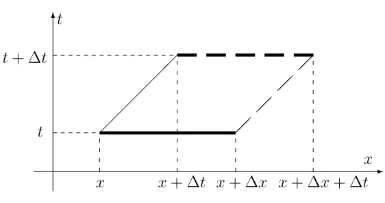
The individuals belonging to the age segment [x;x+ ∆x] at the moment t move along the age scale as the time goes and get into the segment [x+ ∆t;x+ ∆t+ ∆x] at the time t+ ∆t. This suggests a natural parametrization of the introduced family of random variables by means of parallelograms Πx,t∆x,∆t(the upper and the right sides are supposed to be excluded, see figure 1):
∆η = ∆ηx,t∆x,∆t= ∆ηΠx,t∆x,∆t. (1.2)
We will suppose that the following hypothesis holds.
✲ ✻
x t
x x+ ∆t x+ ∆x x+ ∆x+ ∆t t
t+ ∆t
Figure 1. Parallelogram Πx,t ∆x,∆t.
Hypothesis 1. ∆ηΠxk,tk
∆xk,∆tk
, k = 1, . . . , n, n ∈ N, are independent if the parallelograms
Πxk,tk
∆xk,∆tk are pairwise disjoint.
Given arbitrary segments [x;x+ ∆x] and [t;t+ ∆t] consider the uniform partition{xk} of [x;x+ ∆x], where xk = x+k∆x/n, k = 0,1, . . . , n and the corresponding decomposition Πx,t∆x,∆t = Sn−1
k=0Π
xk,t
∆x/n,∆t. The definition of ∆η’s implies the following ”additivity” for them:
∆ηΠx,t∆x,∆t= n−1 X
k=0
∆ηΠxk,t
∆x/n,∆t
Due to the Hypothesis 1it follows
Var h∆ηΠx,t∆x,∆ti= n−1 X
k=0
Var h∆ηΠxk,t
∆x/n,∆t i
.
This condition will be fulfilled if we let
∆ηΠx,t∆x,∆t=
γ√∆x, with probability λ∆t,
0, with probability 1−2λ∆t, −γ√∆x, with probability λ∆t,
(1.3)
for any x, t,∆x,∆t. Hereγ and λare some proportionality factors. This is true since we have
∆ηΠxk,t
∆x/n,∆t
=
γ
r ∆x
n , with probability λ∆t,
0, with probability 1−2λ∆t,
−γ r
∆x
n , with probability λ∆t,
and therefore
Var h∆ηΠxk,t
∆x/n,∆t i
=γ2∆x
n 2λ∆t. (1.4)
Note that the Central Limit Theorem holds for the sequence of series of random variables{ξk(n)}nk=1,
n = 1,2, . . ., where ξk(n) = ∆ηΠxk,t
∆x/n,∆t
, since ξk(n) are independent and identically distributed
with Eξk(n) = 0 and Varξk(n) given by (1.4). By the Central Limit Theorem we conclude that
the distribution of 1
γ√2λ∆x∆t
n X
i=1
ξi(n) converges to standard Gaussian when n → ∞. So, the
Hypothesis 1 together with the additivity property (1) makes it natural to impose the following hypothesis.
Hypothesis 2. ∆ηΠx,t∆x,∆t∼N 0,2λγ2∆x∆t
.
Definition 1. The collection of random variables {Θ(B), B ∈ B(R2)} is called a Gaussian orthogonal measure on the Borel σ-field B(R2) if the following holds:
1. Θ(B)∼N(0, µL(B))for all B ∈ B(R2), where µL is the Lebesque measure of B;
2. B1∩B2 =∅implies Θ(B1) and Θ(B2) are independent for all B1, B2 ∈ B(R2);
3. Θ(∪∞k=1Bk) =Pk∞=1Θ(Bk) (the series is mean square convergent) for any sequence {Bk} ⊂ B(R2) of pairwise disjoint sets.
Hypotheses 1 and 2 imply that ∆η =γ√2λΘ, where Θ is a Gaussian orthogonal measure on B(R2). Thus, equation (1.1) turns into
u(x+ ∆t, t+ ∆t)∆x−u(x, t)∆x =−u(x, t)m(x)∆x∆t+α0u(x, t)Θ
Πxk,t
∆x,∆t
, (1.5)
Definition 2. [1, p. 649] A two-parameter Gaussian random process {B(x, t), x≥0, t≥0} is called a Brownian sheet if it satisfies the following conditions:
1. E[B(x, t)] = 0,for all x, t≥0;
2. Cov (B(x1, t1),B(x2, t2)) = min{x1;x2} ·min{t1;t2} for allx1, x2, t1, t2≥0.
In [4, Definition 12, p. 107] a random process, satisfying the conditions of Definition 2 is called a Wiener–Chentsov random field.
It is easy to see that the random process defined by
B(x, t) := ΘΠ0,0
x,t
, x, t≥0 (1.6)
is a Brownian sheet.
Note that a Brownian sheet on [0; 1]×[0;T] admits the following decomposition
B(x, t) =
n X
n,k=0 θn,k
8√T
π2(2n+ 1)(2k+ 1)sin
π(2n+ 1)t
2T sin
π(2k+ 1)x
2 , (1.7)
where θn,k are independent standard Gaussian random variables, defined on a probability space (Ω,F,P). Replacing ΘΠxk,t
∆x,∆t
in (1.5) by the increment of the Brownian sheet, defined by (1.6) we obtain
u(x+ ∆t, t+ ∆t)∆x−u(x, t)∆x=−u(x, t)∆xµ(x)∆t+
+α0u(x, t) [B(x+ ∆x, t+ ∆t)−B(x, t+ ∆t)−B(x+ ∆x, t) +B(x, t)].
Letu(x, t) be continuously differentiable with respect to x. Then we have
u(x+ ∆t, t+ ∆t)−u(x, t) =u(x, t+ ∆t) +∂u
∂x(x, t+ ∆t)∆t+o(∆t)−u(x, t) =
=u(x, t+ ∆t)−u(x, t) +
∂u
∂x(x, t) +o(1)
∆t+o(∆t) =
=u(x, t+ ∆t)−u(x, t) + ∂u
∂x(x, t)∆t+o(∆t).
Omitting theo(∆t)’s and dividing both sides of the equation by ∆x, we obtain the equation
u(x, t+ ∆t)−u(x, t) =
−∂u∂x(x, t)−µ(x)u(x, t)
∆t+
+α0u(x, t) B
(x+ ∆x, t+ ∆t)−B(x, t+ ∆t)
∆x −
B(x+ ∆x, t)−B(x, t)
∆x
.
(1.8)
2. Difference equation in a Hilbert space
The set of functions ek(x) = √
2 sin x
λk
, k = 0,1, . . ., used in expansion (1.7), where λk = 2
π(2k+ 1) is an orthonormal basis in the space H = L
2[0; 1]. Note that the random processes
βk(t), defined by the series
βk(t) = ∞ X
n=0 θn,k
2√2T π(2n+ 1)sin
π(2n+ 1)t
2T , t∈[0;T], (2.1)
are independent Brownian motions (here, as in (1.7), θn,k are independent standard Gaussian random variables). Thus, we can rewrite the expansion (1.7) as
B(x, t) =
∞ X
k=0
λkβk(t)ek(x) (2.2)
and consider B(t) = B(·, t) as a random process in H. It is easy to see that the series (2.2) is
convergent in L2(Ω,F,P;H) for any t.
Let us introduce the shift operator τ∆x:H→H, defining it on the elements of the basis {ek} by
τ∆xek = sin ∆x
λk ˜
ek+ cos ∆x
λk
ek, (2.3)
where ˜ek(x) := λke′k(x) = √
2 cosλx
k, k = 0,1, . . .. Note that the set {˜ek} is also an orthonormal
basis inL2[0; 1]. Equation (1.8) can be written as the following difference equation in H:
u(t+ ∆t)−u(t) =
−∂x∂ u(t)−mu(t)
∆t+
+α0u(t)
τ∆xB(t+ ∆t)−B(t+ ∆t)
∆x −
τ∆xB(t)−B(t) ∆x
,
whereu(t) =u(·, t).
Definition 3. [6, p. 17] Let H be a Hilbert space. A linear operator X : H → L2(Ω,F,P)
with the properties:
1. X[h]∼N(0,khk2) for any h∈H,
2. X(h1) and X(h2) are independent if (h1, h2)H = 0,
is called a cylindrical standard Gaussian random variable on H.
It follows from the definition that any cylinder standard Gaussian random variable X is a bounded operator: X ∈ L H;L2(Ω,F,P)
with kXk= 1.
Definition 4. [6, p. 19] A family {W(t), t∈R} is called a cylindrical Wiener process if 1. W(t) :H→L2(Ω,F,P) is a linear operator;
2. W(t)[h] is a brownian motion for anyh∈H ;
Let W(t) be a cylindrical Wiener process on a Hilbert space H. It follows from the definition that √1
tW(t) is a cylindrical standard Gaussian random variable on H for anyt >0. We also have that for any orthonormal basis{gk}∞k=0 inH βk(t) :=W(t)[gk] are independent Brownian motions, therefore one can identifyW(t) with the expansion
W(t) = ∞ X
k=0
βk(t)gk (2.4)
by letting
W(t)[h] := ∞ X
k=0
hkβk(t), h= ∞ X
k=0
hkgk ∈H . (2.5)
Although the series (2.4) is divergent in L2(Ω,F,P;H), the right hand side of the equality (2.5)
defines a random variable belonging to L2(Ω,F,P) which can be thought of as a scalar prod-uct (W(t), h)H. Conversely, any sequence of independent Brownian motions {βk(t)}∞k=0 and an
orthonormal basis {gk}∞k=0 inH generate a cylindrical Wiener process onH, defined by (2.5).
The next proposition states that when ∆x → 0, the difference quotients τ∆xB(·, t)−B(·, t) ∆x
converge to a cylindrical Wiener process as cylindrical random variables on the Hilbert space
H=L2[0; 1].
Proposition 1. For anyh∈H
lim
∆x→0E
τ∆xB(t)−B(t)
∆x −W0(t), h 2
H
= 0, (2.6)
where W0(t) is the cylindrical Wiener process, defined by the expansion
W0(t) = ∞ X
k=0
βk(t)˜ek.
P r o o f. Let h =P∞
k=1hkek =P∞k=1˜hke˜k ∈H. Using the expansion (2.2) and the equality (2.3), we obtain
τ∆xB(t)−B(t)
∆x −W0(t), h
H =
∞ X
k=0 βk(t)
h
ζk(∆x)˜hk+γk(∆x)hk i
,
where
ζk(∆x) =
sin ∆x/λk ∆x/λk −
1, γk(∆x) =
cos ∆x/λk−1 ∆x/λk
.
We have
E
τ∆xB(t)−B(t)
∆x −W0(t), h 2
H =t
∞ X
k=0 h
ζk(∆x)˜hk+γk(∆x)hk i2
(2.7)
and due to the estimate
h
ζk(∆x)˜hk+γk(∆x)hk i2
≤2hζk2(∆x)˜h2k+γk2(∆x)h2ki≤4hh˜2k+h2ki,
we conclude that the series in the right hand side of (2.7) is uniformly convergent with respect to ∆x∈R. Since lim
Thus, letting ∆x→0 in (1.8), we arrive at the following difference equation inH:
u(t+ ∆t)−u(t) =
−∂x∂ u(t)−mu(t)
∆t+α0u(t) (W0(t+ ∆t)−W0(t)).
Note, that the last term in the right hand side of this equation can not be thought of as a product of functions of x. This is due to the fact that the increments of the cylindrical Wiener process are cylindrical Gaussian random variables on H and do not belong to H = L2[0; 1] with probability
one. In order to give meaning to the product we rewrite the equation in the following form:
u(t+ ∆t)−u(t) =Au(t)∆t+α0B0(u(t)) (W0(t+ ∆t)−W0(t)), (2.8)
whereA=− d
dx−m(x) :H→H with the domain
D(A) =
u∈H1[0; 1]
u(0) = Z 1
0
b(x)u(x)dx
,
and B0 :H → L(H) is the operator, defined by B0 : u 7→ B0(u), where B0(u) is the operator of
multiplication by u.
Since for any u∈H we have
kB0(u)ekk2H = Z 1
0 |
u(x)ek(x)|2dx≤2kuk2H
and h=P∞
k=0hkek∈H1[0,1] iff khk21 := ∞ X k=0 hk λk 2
<∞, the following estimate holds:
kB0(u)hk2H = ∞ X k=0
hkB0(u)ek 2 H ≤ ∞ X k=0
|hk|kB0(u)ekk !2 ≤ ≤ ∞ X k=0 hk λk 2 ∞ X k=0
λ2kkB0(u)ekk2≤ khk21kuk2H ·2 ∞ X
k=0 λ2k.
SinceP∞
k=0λ2k<∞, it followsB0(u)h∈H. Therefore the equation (2.8) can be understood in the
following weak sense:
(u(t+ ∆t)−u(t), h)H = (u(t), A∗h)H∆t+α0(W0(t+ ∆t)−W0(t))[B0(u(t))h] (2.9)
for any h∈D(A∗). Here A∗h(x) =h′(x)−m(x)h(x) +b(x)h(0) with the domain
D(A∗) =
h∈H1[0; 1] |h(1) = 0 .
Consider the first term in the right hand side of (2.9). We have
(u(t), A∗h)H = (u(t), h′)H −(u(t), mh)H + (u(t),hh, δib)H = = (u(t), h′)H −(m, B0(u(t))h)H + (b, B1(u(t))h)H,
(2.10)
where δ is the Dirac delta-function, considered as an element of the spaceH−1[0; 1], the operator B1 :H → L(H1[0; 1];H) is defined by B1(u)h=hh, δiu, u∈H,h∈H1[0; 1]. The second term in
byb(x) (the mean birth rate) initially contained in the boundary condition, it is natural to introduce an analogous stochastic perturbation of this factor by the termα1(W1(t+ ∆t)−W1(t))[B1(u(t))h],
whereW1(t) is a cylindrical Wiener process independent withW0(t) and α1 is a constant.
Thus, we arrive at the following equation:
u(t+ ∆t)−u(t) =Au(t)∆t+α0B0(u(t)) (W0(t+ ∆t)−W0(t)) + +α1B1(u(t)) (W1(t+ ∆t)−W1(t)),
(2.11)
which is understood in the weak sense, namely:
(u(t+ ∆t)−u(t), h)H = (u(t), A∗h)H∆t+α0(W0(t+ ∆t)−W0(t))[B0(u(t))h]
+α1(W1(t+ ∆t)−W1(t))[B1(u(t))h]
for any h∈D(A∗).
3. Differential equation
For any t > 0 let {tk}Nk=0 be a partition of the segment [0;t], where tk = k∆t, ∆t = t/N. Summing up the equality (2.11) written for the points tk we obtain
u(t)−u(0) = N−1
X
k=0
Au(tk)∆t+ N−1
X
k=0
B0(u(tk)) (W0(tk+1)−W0(tk)) +
+ N−1
X
k=0
B1(u(tk)) (W1(tk+1)−W1(tk)).
LettingN → ∞ we arrive at the following integral Itˆo equation
u(t)−u(0) = Z t
0
Au(s)ds+ Z t
0
B0(u(s))dW0(s) + Z t
0
B1(u(s))dW1(s), (3.1)
if the integrals in the right hand side exist. The equation is usually written in the following differential form:
du(t) =Au(t)dt+B0(u(t))dW0(t) +B1(u(t))dW1(t), u(0) =u0. (3.2)
The necessary condition of existence of the integrals in (3.1) isB0(u), B1(u)∈ L2(H;H) (the space
of Hilbert–Schmidt operators acting in H) for any u ∈ H. It is not the case here, therefore it is impossible to obtain theorems on existence and uniqueness of solution (weak, or mild) for the problem (3.3) (see, for example, Theorem 6.7, p. 164 in [5], Theorem 3.3, p. 97 in [6]).
The way out can be found in setting the problem in the space of generalized Hilbert-space-valued random variables (S)−ρ(H) ⊃ L2(Ω,F, P;H), ρ ∈[0; 1] (see the definition and properties of this space in [9]). It turns out that a cylindrical Wiener process W(t) on H is a differentiable (S)−ρ(H)-valued function of t. Denote its derivative by W(t). It is called a cylindrical singular white noise. It was proved in [3] that for any predictableL2(H, H)-valued process Ψ(t) it holds
Z t
0
Ψ(s)dW(s) = Z t
0
Ψ(s)⋄W(s)ds,
Thus, the problem (3.3) takes the form
du(t)
dt =Au(t) +B0(u(t))⋄W0(t) +B1(u(t))⋄W1(t), u(0) =u0. (3.3)
in the space (S)−ρ(H). The following theorem is stated here without proof as it is a straightforward generalization of the Theorem 3 in [9].
Theorem 1. Let A be the generator of a C0-semigroup of operators in a Hilbert space H,
B0(·), B1(·) ∈ L H,L2(HQ, H)
, where Q is a positive trace class operator in H with the set of eigenvalues {σ2
j}∞j=1 satisfying the condition
X
j
σ−2
j j−2p <∞, for some p∈N,
and HQ = Q1/2(H) with the norm kxkQ = kQ−1/2xkH. Then the problem (3.3) has a unique
solutionu(t)∈(S)−0(H)for anyu0 ∈(D(A)), where(D(A))denotes the domain ofAin(S)−0(H).
Remark 1. Conditions of the theorem hold true for the operators,B and B1 introduced in our
model. To show this, note that the functions σj˜ej(x),j = 0,1,2, . . . form an orthonormal basis in
HQ and for any u∈H=L2[0; 1] we have:
kB(u)k2L2(HQ,H)=X j
kB(u)σje˜jk2= X
j
σj2 Z 1
0
u2(x)˜ej(x)dx≤2 X
j
σ2jkuk2,
kB1(u)k2L2(HQ,H)=X j
kB1(u)σj˜ejk2 = X
j
σ2jh˜ej, δi2kuk2 = 2 X
j
σj2kuk2.
4. Conclusion
Introduction of stochastic perturbation into McKendrick–von Foerster model of an age-struc-tured population requires taking into account certain properties of the oscillations of rates of death and birth. We have shown that the assumption of independence between the random fluctuations of per capita amounts of dead individuals in disjoint segments of the age scale or the time line together with the analogous assumption on the random fluctuations concerning the process of reproduction in the population lead to a difference equation in the Hilbert space L2[0; 1] with a cylindrical
Wiener process. Due to nonregularity of the latter, we finally obtain a model which has the form of an operator-differential equation with cylindrical white noises in the space of generalized Hilbert space-valued random variables satisfying the conditions of the theorem on existence and uniqueness of solutions.
REFERENCES
1. Nasyrov F.S. On the derivative of local time for the Brownian sheet with respect to a space variable. Theory Probab. Appl, 1987. Vol. 32, no. 4. P. 649–658.DOI: 10.1137/1132097
2. Alshanskiy M.A., Melnikova I.V. Regularized and generalized solutions of infinite-dimensional stochastic problems. Sbornik Mathematics, 2012. Vol. 202, no. 11. P. 1565–1592.
DOI: 10.1070/SM2011v202n11ABEH004199
3. Alshanskiy M.A. The Itˆo integral and the Hitsuda-Skorohod integral in the infinite dimensional case. Sib. Elektron. Mat. Izv., 2014. Vol. 11, no. 1. P. 185–199.
5. Da Prato G., Zabczyk J. Stochastic equations in infinite dimensions (2nd edition). Cambridge: Cam-bridge Univ. Press, 2014. 493 p.DOI: 10.1017/CBO9781107295513
6. Gawarecki L., Mandrekar V. Stochastic differential equations in infinite dimensions with applica-tions to stochastic partial differential equaapplica-tions. Berlin, Heidelberg: Springer-Verlag, 2011. 291 p.
DOI: 10.1007/978-3-642-16194-0
7. Ma W., Ding B., Zhang Q. The existence and asymptotic behaviour of energy solutions to stochastic age-dependent population equations driven by Levy processes. Appl. Math. Comput., 2015. No. 256, P. 656–665.DOI: 10.1016/j.amc.2015.01.077
8. Melnikova I.V., Alshanskiy M.A. The generalized well-posedness of the Cauchy problem for an abstract stochastic equation with multiplicative noise.Proc. Steklov Inst. Math., 2013. Vol. 280 (Suppl. 1), P. 134– 150.DOI: 10.1134/S0081543813020119
9. Melnikova I.V., Alshanskiy M.A. Stochastic equations with an unbounded operator coefficient and multi-plicative noise.Sib. Math. Journ., 2017. Vol. 58, no. 6. P. 1052–1066.DOI: 10.1134/S0037446617060143
10. Qi-Min Z., Wen-An L., Zan-Kan N. Existence, uniqueness and exponential stability for stochas-tic age-dependent population. Appl. Math. Comput., 2004. Vol. 154, no. 1. P. 183–201.