RPIM and RPIM-MLS based MDLSM method for the solution of elasticity problems

Sharif University of Technology

Transactions A: Civil Engineering www.scientiairanica.com

RPIM and RPIM-MLS-based MDLSM method for the

solution to elasticity problems

S. Nikravesh

_{, M.H. Afshar}

_{and S. Faraji}

a. School of Civil Engineering, Iran University of Science and Technology, Narmak, Tehran, Iran.

b. Department of Civil & Environmental Engineering, Amirkabir University of Technology, 424 Hafez Ave, Tehran, Iran. Received 17 November 2014; received in revised form 4 August 2015; accepted 19 October 2015

KEYWORDS Mesh-free method; MDLSM method; Radial Point

Interpolation Method (RPIM);

Moving Least-Squares approximation (MLS); Coupled method.

Abstract. One of the main diculties in the development of meshless methods using the Moving Least-Squares approximation, such as Mixed Discrete Least-Squares Meshless (MDLSM) method, is the imposition of the essential boundary conditions. In this paper, the RPIM shape function, which satises the properties of the Kronecker delta condition, is employed in the Mixed Discrete Least-Squares Meshless (MDLSM) method for solving the elasticity problems. Accordingly, two new MDLSM formulations are proposed in this article, namely RPIM-based MDLSM and coupled MLS-RPIM MDLSM formulation. The essential boundary conditions can be imposed directly on the both presented methods. The proposed methods are used for the solution of three benchmark elasticity problems, and the results are presented and compared with the available analytical solutions and those of MLS-based MDLSM formulations. In addition, in each example, dierent types of nodal distributions, uniform, and rened congurations are considered to test the performance of the presented methods. The numerical tests indicate higher accuracy of the suggested approaches in comparison with the MLS-based MDLSM method.

© 2016 Sharif University of Technology. All rights reserved.

1. Introduction

In the past decades, a group of so-called meshless or mesh-free methods has become one of the hottest areas of research in computational mechanics. The main objective of meshless methods is to alleviate the constrained structure of the mesh and to construct the approximation entirely in terms of nodes. Various meshless methods have been introduced and developed to solve dierent PDE problems that cannot be easily treated by traditional Finite Element Method (FEM). Some of the well-known meshless methods can be listed here such as Diuse Element Method (DEM) [1], the Element-Free Galerkin (EFG) method [2], the point

*. Corresponding author.

E-mail addresses: [email protected] (S. Nikravesh); [email protected] (M.H. Afshar); [email protected] (S. Faraji)

interpolation meshless method based on radial basis functions (RPIM) method [3], the Reproducing Kernel Particle Meshless (RKPM) method [4], Moving Particle Semi-implicit (MPS) method [5], and Meshless Local Petrov-Galerkin (MLPG) method [6].

A Discrete Least-Squares Meshless method (DLSM) was proposed by Arzani and Afshar [7] to solve the elliptic problems. Unlike the EFG method which requires background mesh for numerical integration procedure, this method did not involve any integration procedure; therefore, it did not need any background mesh. The method was later extended to simulate free surface problems [8]. The Collocated Discrete Least-Squares Meshless (CDLSM) [9,10] method was later proposed to improve the accuracy of the DLSM method and used to solve elasticity and uid ow problems. A Mixed Discrete Least-Squares Meshless (MDLSM) method has been recently introduced [11,12] for an eective solution to planer elasticity problems.

Furthermore, a number of robust, adaptive renement techniques have been recently presented in order to improve the eciency of the MDLSM method [13-15]. The original DLSM and MDLSM method use the Moving Least-Squares (MLS) approximation to construct shape functions. One of the main diculties in the implementation of MLS-based meshless ap-proaches, such as MDLSM method, is the imposition of the essential boundary conditions since the MLS shape functions, in general, do not satisfy the Kronecker delta condition. Therefore, the essential boundary conditions cannot be directly enforced in the MDLSM method. For this, the penalty method [11] has been used to impose the essential boundary conditions on MDLSM approach. The penalty coecient must be chosen large enough in order to impose the boundary conditions, but it should not exceed the maximum value so that it could avoid ill-posed coecient ma-trices. This maximum value is dierent depending on machines precision and numerical method used.

The radial point interpolation shape functions (RPIM) was employed by GR Liu and Gu in mesh-free weak-form methods [3,16]. The major advantage of RPIM is that the shape function possesses the Kronecker delta properties paving the way for easier implementation of the essential boundary conditions. Recently, a coupled EFG-RPIM method is proposed to resolve the problem of enforcing the essential boundary conditions in EFG method using RPIM approxima-tion [17].

In this paper, the RPIM shape functions are employed in the MDLSM method to solve the elas-ticity problems. In order to use RPIM in MDLSM formulation, two dierent approaches are proposed in this article. In the rst approach, the unknown nodal parameters are approximated using the RPIM shape functions; in the second approach, coupled MLS-RPIM shape functions are used in which the RPIM approxi-mation is only applied to the boundary nodes with the MLS shape functions used for the interior nodes. Both formulations allow for direct imposition of the essential boundary conditions removing the need for the penalty method. Performances of the proposed methods are tested by three benchmark examples from the literature on regular and adapted nodal distributions, and the results are presented and compared with those of available analytical solutions. The results indicate the superior accuracy of the proposed methods compared to the conventional MDLSM. Furthermore, it is shown that the RPIM-based formulation is more exible and accurate than the conventional and coupled MLS-RPIM formulation on the adapted nodal arrangements, while the coupled MLS-RPIM formulation shows a better performance than the RPIM-based formulation on the regular nodal distributions.

The layout of the paper is as follows. In Section

2, the RPIM shape function is introduced. The orig-inal MDLSM and proposed formulations using RPIM approximation for solving elasticity problems are given in Section 3. The numerical results are presented in Section 4. And, nally, some concluding remarks are addressed in Section 5.

2. Meshless shape functions

Several techniques have been developed to construct shape functions for meshless methods [16]. In this section, the RPIM shape function, used in the proposed approaches, is presented as follows:

2.1. Radial point interpolation shape functions (RPIM)

The RPIM was employed by GR Liu and Gu in weak-form meshless methods [3,16]. In this method, the unknown function (X) is approximated by:

(X) =

n

X

i=1

Ri(X)ai+ m

X

j=1

Pj(X)bj= RT(X)a

+ PT_{(X)b; (1)}

with the constraint condition as:

n

X

i=1

Pj(Xi)ai = 0 (j = 1; 2; :::; m); (2)

where ai and bj are the unknown interpolation

con-stants, m is the number of polynomial basis functions, Pj(X) is monomial in the space coordinate X = (x; y),

n is the number of nodes in the support domain of point X, and Ri(X) is the Radial Basis Function (RBF).

There are many types of radial basis functions. In this paper, Multi-Quadrics Radial Basis Function (MQ-RBF) is employed as follows:

Ri(X) = (ri2+ (dc)2)q; (3)

where dc is the characteristic length attributed to the

nodal distribution, and q are the RBF dimensionless shape parameters, and ri = p(x xi)2+ (y yi)2.

The shape parameters of MQ-RBF can highly aect the performance of the RPIM approximation. In this paper, value q = 1:03 is used, which was suggested by Wang and Liu [18]. Preliminary numerical tests on dierent examples indicated that the value of = 3 leads to better results in the analysis of the 2D elasticity problems by MDLSM method.

Constants aiand bjin Eq. (1) are then determined

by enforcing Eq. (1) to be satised at n nodes in the inuence domain of point X. Eqs. (1) and (2) can be re-written in matrix form as:

where: CT_=a

1 a2 ::: an b1 b2 ::: bm_1(n+m);

T =1 2 ::: n 0 0 ::: 0_1(n+m):

And, the matrix G in Eq. (4) is dened as follows:

G =

R0 Pm

PT

m 0

(n+m)(n+m)

; (5)

where R0and Pm are dened as:

R0=

2 6 6 6 4

R1(r1) R2(r1) Rn(r1)

R1(r2) R2(r2) Rn(r2)

... ... ... ... R1(rn) R2(rn) Rn(rn)

3 7 7 7 5 nn ; (6) and: PT m = 2 6 6 6 6 6 4

1 1 1 x1 x2 xn

y1 y2 yn

... ... ... ... Pm(x1) Pm(x2) Pm(xn)

3 7 7 7 7 7 5 mn (7)

Since the matrix R0 is symmetric, the matrix G will

also be symmetric. Eq. (1) can be re-written using Eq. (4) as follows:

(X) = RT_{(X)a + P}T_{(X)b =R}T_{(X) P}T_(X)C

! (X)=RT_{(X) P}T_(X)G 1_{; (8)}

where the RPIM shape functions can be shown as:

NT_{(X) =R}T_{(X) P}T_(X)G 1

= [N1(x) N2(x) Nn(x) Nn+1(x)

Nn+m(x)]: (9)

Hence, the RPIM shape functions corresponding to the n unknown nodal values are obtained as:

NT_{(X) =N}

1(x) N2(x) Nn(x): (10)

The RPIM shape functions can be calculated in an alternative form by solving Eq. (4) and substituting the solution into Eq. (1):

NT_{(X) = R}T_(X)G

a+ PT(X)Gb

=N1(x) N2(x) Nn(x): (11)

where:

Gb= (PmTR0 1Pm) 1PmTR0 1; (12)

and:

Ga = R0 1(Inn PmGb): (13)

The RPIM shape functions pass through the nodal values. Therefore, RPIM shape functions, given in Eq. (10), possess the Kronecker delta property.

More detailed information on the RPIM approxi-mation and the Radial Basis Functions (RBF) can be found elsewhere [3,16,18,19].

3. Mixed discrete least-squares meshless method for elasticity

The conventional MDLSM and proposed formulations using RPIM approximation for solving elasticity prob-lems are given in this section.

3.1. MLS-based MDLSM formulation

Consider the following partial dierential equation governing 2D linear elasticity problems [20]:

u ( + )r(r:u) = f in ; (14) with the following displacement and traction boundary conditions: 8 > < > :

u = u

on u

v = v

8 > < > :

xnx+ xyny = tx

on t

xynx+ yny= ty

(15)

where is the problem domain that incorporates an elastic material; t and u are the traction and

displacement boundaries, respectively; nx and ny are

direction cosines of the normal to the boundary; t x, ty

and u_{, v are components of the prescribed tractions}

and displacements in the Cartesian coordinate system, respectively.

The parameters and are the Lame constants dened for plain stress problems as:

= _{(1 2v)(1+v)}Ev >0 and = _{2(1 + v)}E >0; (16) where E is the elasticity modulus and v is the Poisson ratio.

In addition, stresses can be dened in terms of the displacement components as follows:

x= ( + 2)@u_@x+ _@y@v;

y = @u_@x+ ( + 2)@v_@y;

xy= @u @y + @v @x : (17)

Rewriting Eq. (14) in terms of stresses leads to: @x

@x + @xy

@y = fx in ; @xy

@x + @y

@y = fy in : (18) Eqs. (17) and (18) can be rewritten in a matrix form as follows:

S() + F = 0; (19) where and F are vectors of unknowns and forcing terms dened as:

=u v x y xyT; (20)

F =0 0 0 fx fyT: (21)

And, S(:) is the rst-order dierential operator dened as:

S(:) = S1(:)x+ S2(:)y+ S3(:); (22)

where S1, S2, and S3 are dened by the following

matrices:

S1=

2 6 6 6 6 4

( + 2) 0 0 0 0 0 0 0 0 0 0 0 0 0 0 1 0 0 0 0 0 0 1 3 7 7 7 7 5;

S2=

2 6 6 6 6 4

0 0 0 0 0 ( + 2) 0 0 0 0 0 0 0 0 0 0 0 1 0 0 0 1 0 3 7 7 7 7 5;

S3=

2 6 6 6 6 4

0 0 1 0 0 0 0 0 1 0 0 0 0 0 1 0 0 0 0 0 0 0 0 0 0

3 7 7 7 7

5: (23)

The boundary conditions of Eq. (15) are also re-written in a matrix form as:

D F_{= 0; (24)}

where F _{and D are dened as:}

F_{=u v t}

x ty; (25)

and: D = 2 6 6 4

1 0 0 0 0 0 1 0 0 0 0 0 nx 0 ny

0 0 0 ny nx

3 7 7

5 : (26)

The residuals at the typical node i can be dened as: Ri = (S)i+ Fi in ; (27)

R i = (D)i Fi on : (28)

A least-squares functional for typical node i can, therefore, be dened using penalty approach:

Ii= (RTR)i+ (RTR )i: (29)

And, the least-squares functional for the whole domain can be dened as:

IM ₌Xn i=1

(RT

R)i+ n

X

i=1

(RT_{5R )}

i; (30)

where condition is the penalty coecient that should be large enough to satisfy the boundary desired accu-racy. nand n are the number of nodes in the domain

and on the boundaries, respectively.

Minimizing the least-squares functional with re-spect to the vector of unknown nodal parameters leads to:

K = F; (31)

where:

Klm = n

X

i=1

[S(Nl)]Ti [S(Nm)]i+

n

X

i=1

[D(Nl)]Ti [D(Nm)]i; (32)

and:

Fl= n

X

i=1

[S(Nl)]Ti Fi+ n

X

i=1

[D(Nl)]Ti Fi; (33)

where Nl is the MLS shape function [11] of node l. It

can be noted that the MLS approximation generally does not pass through the nodal values. Thus, the MLS shape functions do not satisfy Kronecker delta condition.

More detailed explanations of this shape function can be found elsewhere [11,16].

3.2. Proposed RPIM-based MDLSM formulation

In this approach, the unknown parameters are approx-imated using the RPIM shape functions. Since RPIM satises Kronecker delta property, the displacement boundary conditions can be imposed as conveniently as in conventional FEM, and there is no need for using the penalty method. The stress boundary conditions are enforced via the least-squares functional as follows.

The least-squares functional for the whole domain is dened as:

IR₌Xn i=1

(RT

R)i+ n

X

i=1

(RT_{R )}

i; (34)

where the residuals Rand R are dened in Eqs. (27)

and (28). Minimizing the least-squares functional with respect to the vector of unknown nodal parameters leads to:

K = F; (35)

where:

Klm= n

X

i=1

h S( ~Nl)

iT i

h S( ~Nm)

i i+ n X i=1 h D( ~Nl)

iT i

h D( ~Nm)

i

i; (36)

and:

Fl= n

X

i=1

h S( ~Nl)

iT i Fi+

n

X

i=1

h D( ~Nl)

iT i F

i; (37)

where ~Nl is the RPIM shape function of node l. The

nal stiness matrix K is square (5N 5N), symmetric and positive-denite matrix in which N is the total number of nodes.

3.3. Proposed MDLSM formulation using coupled MLS-RPIM shape functions Consider an arbitrary support domain containing n typical nodes. As shown in section two, MLS ap-proximation requires the solution of m m linear equation system, while n n linear system should be solved in the RPIM method, where m is the monomial basis functions. Generally, n is much bigger than m; therefore, the computing eort of RPIM is, in general, more than MLS.

In this section, an alternative approach is pro-posed in order to avoid increased computational cost of solving large-scale problems while improving the eciency of the boundary condition imposition on MDLSM method. In this approach, coupled MLS-RPIM shape functions are used to approximate the trail functions in which the MLS shape functions are used for the nodes inside the problem domain, and the RPIM approximation is only applied to the boundary nodes. Therefore, The displacement bound-ary conditions are imposed directly, and the stress boundary conditions are applied via the least-squares functional. This requires the following modications in the conventional formulation.

In the proposed approach, the least-squares func-tional is formed as Eq. (34) leading to the matrices

Klm and Fl dened by Eqs. (35)-(37), with the shape

function ~N dened by the following condition: If i 2 fn g ! ~N = NRPIM

Else ! ~N = NMLS_{; (38)}

where NRPIM_{and N}MLS_{are the RPIM and MLS shape}

functions, respectively.

The nal stiness matrix K is square (5N 5N), symmetric and positive denite matrix in which N is the total number of nodes.

4. Numerical examples

In this section, three benchmark examples from elas-ticity with analytical solution are solved using the pro-posed RPIM-based MDLSM, MDLSM using coupled RPIM shape functions, and the original MLS-based MDLSM approaches on uniform and adapted nodal distributions. The results are presented and compared with the available exact solutions. It should be noted that all the adapted congurations are made manually by the engineering judgments. The examples include:

1. Cantilever beam;

2. Cylinder subjected to internal pressure;

3. Innitive plate with a circular hole.

In this paper, a normalized value of least-squares functional is used as the residual error estimator in which the total residual error eg is dened as:

eg=

p I q

T; (39)

where I is the value of least-square functional dened in Eqs. (30) and (34) for each proposed method, and is the vector of unknowns.

Furthermore, in all problems, the second order polynomial basis (P = 2; m = 6) is used to construct MLS shape functions. The radius of the support domain of node i is calculated as follows:

dw= dm; (40)

where dmis the distance of mth nearest node to point

i, m is the number of terms used in polynomial basis P (m = 3 for linear polynomial basis and m = 6 for quadratic polynomial basis), and is a constant coecient that varies between 2 to 3 determined by a trail-and-error procedure. Penalty coecient used in MLS-based MDLSM method is taken to be = 108_.

All the problems are solved on an Intel(R) Core(TM)2 Duo T9550 Machine with 2.67GHz CPU

Figure 1. A cantilever beam subjected to load at the end.

4.1. Example 1: Cantilever beam

A cantilever beam subjected to a concentrated load at the free end (Figure 1) is considered as the rst example. The analytical solution of this example is available [20] as follows:

u = _6EJP y 3x(2L x) + (2 + v)(y2 _c2_);

V = _6EJP x2_{(3L x) + 3vy}2_{(L x) + (4 + 5v)c}2_x

xx= P(L x)y_J ;

yy = 0;

xy =_2JP c2 y2; (41)

where L is the length of the beam, v is the Poisson's ratio, and J is the moment of inertia of the rectangular cross-sectional beam with the unit thickness dened as J = 2c3_{=3. This example is solved using the proposed}

approaches and original MDLSM method under the plane stress condition with the following constraints: P = 1, E = 1000, v = 0:25, L = 8, and c = 1.

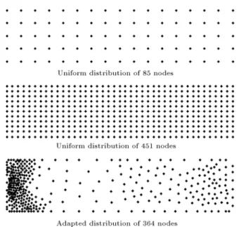
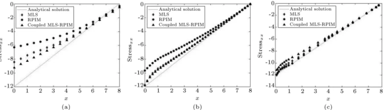
In this example, two uniform nodal distributions of 85 and 451 nodes and an adapted conguration containing 364 nodes are considered for solving this problem, as shown in Figure 2. The results are presented and compared in Table 1. In addition, the variation of stress xx along the upper boundary

and the horizontal displacement ux along the bottom

boundary are plotted for each nodal distribution (Fig-ures 3 and 4). As seen from the results, the MDLSM method using coupled shape functions produces more accurate results on uniform congurations, while the RPIM-based MDLSM has been able to produce more accurate results on the adapted distributions.

Figure 2. Three nodal congurations (Example 1).

4.2. Example 2: Cylinder subjected to internal pressure

The second example considered in this paper is a cylinder subjected to internal pressure (Figure 5). Due to the symmetry, just a quarter of the cylinder is simulated. The analytical solution of this problem [20] is:

r= r 2 1P

r2 2 r21

1 r22

r2

; (42)

= r 2 1P

r2 2 r21

1 + r22

r2

: (43)

The boundary conditions are shown in Figure 6. This example is solved using the proposed methods with r1 = 1, r2 = 5, P = 1, v = 0:3, and E = 1 under

the plane stress condition.

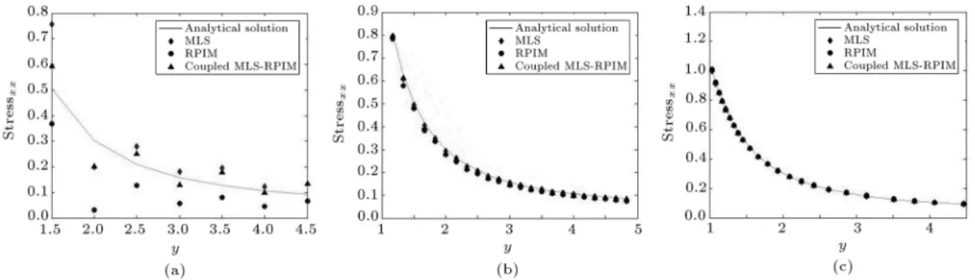
Once again, two uniform nodal distributions of 106 and 765 nodes and an adapted conguration containing 481 nodes are considered for solving this problem, as shown in Figure 7. The results are presented and compared in Table 2. Furthermore, the variation of stress xx along x = 0 and y =

0 boundaries is plotted for each nodal arrangements (Figures 8 and 9). The results illustrate the accuracy of using RPIM shape functions in the MDLSM method.

Table 1. Comparison of total residual errors in Example 1.

Total residual error

Nodal distribution Uniform Uniform Adapted

Total number of nodes 85 451 364

Shape functions

MLS 0.0158 0.0050 0.0028

RPIM 0.0161 0.0040 8.0710 4

Figure 3. Normal stress xxalong y = 1 (Example 1): (a) Coarse uniform distribution with 85 nodes; (b) ne uniform

distribution with 451 nodes; and (c) rened distribution with 364 nodes.

Figure 4. Vertical displacement v along y = 1 (Example 1): (a) Uniform distribution with 85 nodes; (b) uniform distribution with 451 nodes; and (c) adapted distribution with 364 nodes.

Figure 5. A cylinder subjected to internal pressure. Figure 6. A quarter of the cylinder and its boundary.

Table 2. Comparison of total residual errors in Example 2.

Total residual error

Nodal distribution Uniform Uniform Adapted

Total number of nodes 106 765 481

Shape functions

MLS 0.1931 0.0095 0.0011

RPIM 0.2003 0.0109 4.3210 4

Figure 7. Three nodal congurations (Example 2).

Figure 8. Normal stress xxalong y = 0 (Example 1): (a) Uniform distribution with 106 nodes; (b) uniform distribution

with 765 nodes; and (c) adapted distribution with 481 nodes.

Figure 9. Normal stress xxalong x = 0 (Example 1): (a) Coarse uniform distribution with 106 node; (b) ne uniform

distribution with 765 nodes; and (c) rened distribution with 481 nodes.

4.3. Example 3: Innite plate with a circular hole

The nal example considered in this paper is an innitive plate with a circular hole subjected to a uniaxial traction (t), as shown in Figure 10. The analytical solution for this example is available [20] as follows:

ur= _4Gt

r

! 1

2 + cos(2)

+r_r2 1 + 55(1 + !) cos(2) _rr4₃cos(2)

;

u= _4Gt

(1 !)r_r2 r r_r4₃

sin(2);

xx=t

1 r_r2₂

3

2cos(2)+cos(4)

+3r_2r4₄ cos(4)

;

yy=

_r2 r2

₁

2cos(2) cos(4)

+3r_2r4₄cos(4)

;

xy= t

r2

r2

1

2sin(2)+sin(4)

3r4

2r4sin(4)

; (44)

Figure 10. An innite plate with a circular hole under a uniaxial load t.

Figure 11. Uniform and adapted nodal congurations (Example 3).

where G is the shear modulus, ! = (3 v)=(1 + v), and v is the Poisson's ratio.Due to the symmetry, the problem is solved using only a quarter of the plate with the dimension of 5r where r is the radius of the hole.

The symmetry boundary conditions are imposed on the bottom and left boundaries; no traction boundary condition is applied at the hole boundary, and the traction boundary conditions are imposed on the top and right boundaries. This example is solved using t = 1, E = 1000, and v = 0:3 under the plane stress condition.

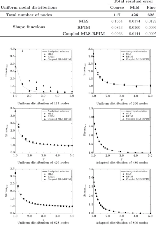
This example is solved considering three uni-form distributions of 117, 426, and 628 nodes and another three adapted distributions of 260, 480, and 809 nodes (Figure 11). The normal stress, xx,

along x = 0 boundary is shown for each nodal arrangement (Figure 12). The residual errors are also compared in Tables 3 and 4. As can be seen from the results, the coupled MLS-RPIM based MDLSM has produced more accurate results on the uniform nodal distributions, while the RPIM-based-MDLSM shows superior performance on the rened congura-tions.

5. Conclusion

In this paper, the RPIM shape functions are used in the MDLSM method to solve elasticity problems. Two dierent approaches are suggested to incorporate RPIM in MDLSM formulation, namely the RPIM-based MDLSM and the coupled MLS-RPIM-RPIM-based MDLSM formulation. In both approaches, the es-sential boundary conditions can be imposed directly removing the need for penalty methods. The pro-posed methods were used for the solution of three benchmark elasticity problems, and the results are presented and compared with the available analytical solutions and those of MLS-based MDLSM formula-tion. Uniform and adapted congurations of dier-ent scales are also considered to test the eciency and reliability of the presented methods. The re-sults indicated that both suggested approaches are, in general, more accurate than the MLS-based formu-lation. Furthermore, the coupled MLS-RPIM-based MDLSM has indicated more accuracy on the uniform nodal distributions, while the RPIM-based MDLSM has shown more accuracy on the rened congura-tions.

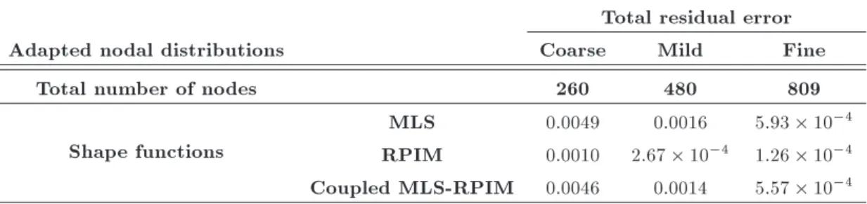
Table 3. Comparison of total residual error for adapted nodal congurations in Example 3. Total residual error

Adapted nodal distributions Coarse Mild Fine

Total number of nodes 260 480 809

Shape functions

MLS 0.0049 0.0016 5:93 10 4

RPIM 0.0010 2:67 10 4 _{1:26 10} 4

Table 4. Comparison of total residual error for uniform nodal congurations in Example 3. Total residual error

Uniform nodal distributions Coarse Mild Fine

Total number of nodes 117 426 628

Shape functions

MLS 0.1654 0.0174 0.0128

RPIM 0.0843 0.0160 0.0096 Coupled MLS-RPIM 0.0963 0.0144 0.0095

Figure 12. Normal stress xxalong x = 0 (Example 3).

References

1. Nayroles, B., Touzot, G. and Villon, P. \The diuse elements method", Comptes Rendus De L Academie Des Sciences Serie Ii, 313(2) pp. 133-138 (1991).

2. Belytschko, T., Lu, Y.Y. and Gu, L. \Element-free Galerkin methods", International Journal for Numer-ical Methods in Engineering, 37, pp. 229-256 (1994).

3. Wang, J. and Liu, G. \A point interpolation meshless

method based on radial basis functions", Interna-tional Journal for Numerical Methods in Engineering, 54(11), pp. 1623-1648 (2002).

4. Liu, W.K., Jun, S. and Zhang, Y.F. \Reproducing kernel particle methods", International Journal for Numerical Methods in Fluids, 20(8-9), pp. 1081-1106 (1995).

semi-implicit method for fragmentation of incompressible uid", Nuclear Science and Engineering, 123(3), pp. 421-434 (1996).

6. Atluri, S. and Zhu, T. \A new meshless local Petrov-Galerkin (MLPG) approach in computational mechan-ics", Computational Mechanics, 22(2), pp. 117-127 (1998).

7. Arzani, H. and Afshar, M. \Solving Poisson's equations by the discrete least square meshless method", WIT Transactions on Modelling and Simulation, 42, pp. 23-31 (2006).

8. Shobeyri, G. and Afshar, M. \Simulating free sur-face problems using discrete least squares meshless method", Computers & Fluids, 39(3), pp. 461-470 (2010).

9. Afshar, M. and Lashckarbolok, M. \Collocated discrete least-squares (CDLS) meshless method: Error esti-mate and adaptive renement", International Journal for Numerical Methods in Fluids, 56(10), pp. 1909-1928 (2008).

10. Firoozjaee, A.R. and Afshar, M.H. \Discrete least squares meshless method with sampling points for the solution of elliptic partial dierential equations", Engineering Analysis with Boundary Elements, 33(1), pp. 83-92 (2009).

11. Amani, J., Afshar, M.H. and Naisipour, M. \Mixed discrete least squares meshless method for planar elasticity problems using regular and irregular nodal distributions", Engineering Analysis with Boundary Elements, 36(5), pp. 894-902 (2012).

12. Faraji, S., Afshar, M.H. and Amani, J. \Mixed discrete least square meshless method for solution of quadratic partial dierential equations", Scientia Iranica, 21(3), p. 492 (2014).

13. Afshar, M.H., Amani, J. and Naisipour, M. \A node enrichment adaptive renement in discrete least squares meshless method for solution of elasticity prob-lems", Engineering Analysis with Boundary Elements, 36(3), pp. 385-393 (2012).

14. Afshar, M.H., Naisipour, M. and Amani, J. \Node moving adaptive renement strategy for planar elas-ticity problems using discrete least squares meshless method", Finite Elements in Analysis and Design, 47(12), pp. 1315-1325 (2011).

15. Nikravesh Kazeroni, S. and Afshar, M.H. \An adaptive node regeneration technique for the ecient solution of elasticity problems using MDLSM method", Engineer-ing Analysis with Boundary Elements, 50, pp. 198-211 (2015).

16. Liu, G.-R. and Gu, Y.-T., An Introduction to Meshfree Methods and Their Programming, Springer (2005).

17. Cao, Y., Yao, L. and Yin, Y. \New treatment of essential boundary conditions in EFG method by coupling with RPIM", Acta Mechanica Solida Sinica, 26(3), pp. 302-316 (2013).

18. Wang, J. and Liu, G. \On the optimal shape param-eters of radial basis functions used for 2-D meshless methods", Computer Methods in Applied Mechanics and Engineering, 191(23), pp. 2611-2630 (2002).

19. Liu, G.-R., Meshfree Methods: Moving Beyond the Finite Element Method, Taylor & Francis (2009).

20. Timoshenko, S. and Goodier, J., Theory of Elasticity, 3rd Edition, New York: McGraw-Hill (1970).

Biographies

Siavash Nikravesh Kazeroni was graduated from Iran University of Science and Technology (IUST), Tehran, Iran, in late 2014, and received his master's degree in Civil Engineering-Hydraulic Structures ma-jor. His MS research focused on numerical analysis and mesh-free methods. This study was also presented as his master's seminar at IUST. Currently, he is pursuing his education and studying PhD in the University of New Mexico (UNM), NM, USA. His research elds consist of computational engineering, simulation, and structural analysis.

Mohammad Hadi Afshar obtained his BS degree in Civil Engineering from University of Tehran, Iran, and his MS and PhD degrees in University College of Swansea, Wales, UK. He is now an Associate Professor in the Civil Engineering Department at Iran University of Science and Technology (IUST), Tehran, Iran. His research interests include numerical modeling of solid and uid mechanic problems and optimization methods.

Saeb Faraji received his MSc degree in Hydraulic Structures from Iran University of Science and Tech-nology (IUST). Now, he is a PhD student in Amirk-abir University of Technology working on mesh-free methods. His research interests include numerical simulation procedures focusing on mesh-free and nite element methods and their applications in elasticity and uid problems.