Dithmarschen Bight
M. Rahbani
Department of Oceanic and Atmospheric Science, University of Hormozgan, Bandar-Abbas, Iran. Received 29 November 2012; received in revised form 18 August 2013; accepted 15 October 2013
KEYWORDS Suspended; Sediment; Concentration; Model; Critical; Shear; Stress; Tide.
Abstract.The main concern of this investigation is to evaluate the ability of the Delft3D-ow package in studying the distribution of Suspended Sediment Concentration (SSC) over the depth in the Dithmarschen Bight. The area consists of tidal channels and tidal ats, with a prevailing semi-diurnal tide, and is tidally dominated. Required eld data were prepared using the data collected by a transmissometer and a mechanical sampler. A factor of two of the measured SSC was used to evaluate the performance of the model, and some dissimilarity was found between the modeled and measured SSC. To verify the reason, two comparing procedures were carried out. First, evolutions of the vertical prole of the SSC from the model and the eld were prepared and compared. In another procedure, snapshots of the distribution of SSC during dierent phases of a tidal cycle were prepared for both model results and eld data. It was found that the predicted SSC values are in good agreement with eld data during the periods of ood phase and low slack water. However, spatial dissimilarities are observed during the periods of high slack water and the ebb phase. An insucient supply of sediment from the tidal at predicted by the model was considered to be responsible.
c
2014 Sharif University of Technology. All rights reserved.
1. Introduction
Coastal zones have a high potential for numerous physical activities and are of critical economic im-portance. They encompass immense environmental, social and economic value, and, therefore, should be managed ecologically, ethically and economically. To achieve this aim, it requires a thorough understanding of the physical, chemical, biological and other processes involved. Among the physical processes is sediment transport.
Observations and eld measurements are neces-sary but insucient to describe these processes
pre-*. Tel.: +98 9376383087; Fax: +98 7617660032
E-mail address: [email protected] (M. Rahbani)
cisely, because of the size and nature of the area involved. The choices are numerical and computational techniques. These models involve the simulation of ow and sediment transport conditions based on the for-mulation and solution of mathematical relationships. When these models and the relevant computational techniques are established, they can be improved and rened as more data and additional or rened param-eters become available. The task is to improve our understanding of their limitations and constraints, as well as knowledge of the physical processes involved.
The application of models in coastal engineering is reasonably advanced in terms of the prediction of ow hydrodynamics, but it is imprecise in the prediction of sediment transport and morphodynamics. The lack of sucient and adequate eld data, on the one hand,
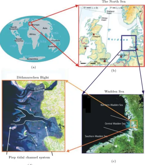
Figure 1. Geographical location of central Dithmarschen Bight.
and the lack of universally accepted equations and parameters, on the other, make prediction of sediment transport a challenging topic [1]. The main purpose of this study is to evaluate the predictive ability of a model developed using the Delft3D package to predict sediment dynamics for the coastal zone of Central Dithmarschen Bight, which is located on the German North Sea, as shown in Figure 1. The 3D ow model, incorporated with the sediment module of the package, was used for this investigation. The model results were compared with eld data to investigate the performance of the model, with the main interest in the prediction of SSC, in order to nd the reason or reasons for the weak correlation existing between model results and eld data.
2. Area under investigation
Dithmarschen Bight is located between the Eider and Elbe estuaries and situated about 100 km north of Hamburg (Figure 1(c)). It consists of tidal channels, tidal ats and sand banks. It is tidally dominated and known as a well-mixed body of water with a
mean tidal range of about 3.2 m. The most dominant morphological features of the area are tidal ats, tidal channels and sand banks over the outer region. Under moderate conditions, the maximum mean water depth in the tidal channels is about 18m, and approximately 50% of the domain falls dry at low tide. The tidal ats and sandbanks are exposed at low water [2]. The most dynamic morphological units are found at the western boundary of the tidal ats, where wave action interferes with strong tidal and wind driven currents [3]. The banks and shoals in this region exhibit the highest migration rates. The sediments in suspension are mainly cohesive, consisting of very ne to medium-grain silt [4].
The specic area under investigation in this re-search is the Piep tidal channel system, which is part of Dithmarschen Bight, and is shown in Figure 1(d). It consists of two main channels, namely, Norderpiep and Suderpiep. These two channels conjunct together to form the Piep channel near the land on the tidal at. The width of the channels and their rivulets (ending the tidal ats or the shore) varies spatially and temporally from a few meters to about 4 km.
Figure 2. Locations of the cross sections in investigation and the position of monitoring points.
3. Material and methods
To obtain reliable results from the models, a compre-hensive knowledge of the processes involved is nec-essary but insucient. Precise values of parameters and variables derived on the basis of adequate eld measurements are also needed to establish the model and, also, for the purpose of model calibration and validation.
The required eld data for this study were col-lected from \Prediction of Medium Term Coastal Mor-phodynamics", known as the PROMORPH project. It was executed during the period May 1999 to June 2002. The data were collected using equipped cruising vessels under dierent conditions.
The eld data used in this study cover two cross sections in the two channels: Norderpiep (T1), and Piep (T2) (see Figure 2). Each time, the cruises were carried out across cross sections T1 and T2 for one full tidal cycle. In each measuring campaign, current velocity and SSC were collected at several stations
across the width of each cross section and at various depths of each station.
As seen in Figure 2, cross section T1 is in the northern channel, and it is quite narrow with a width of 770 meters and a depth of 2.8 to 16.1 meters. Cross section T2 is in the Piep channel, which is ended over the tidal at area. The width of this cross section is about 1200 meters and its depth is between 6.2 and 17.9 meters. The date of the surveys, corresponding tidal range, period of measuring cruises, and the number of stations where the measurements were carried out, are summarized in Table 1. The boundaries of the model have been chosen far from the area of interest, namely, the Piep tidal system. This has ensured that the boundary conditions will not aect the hydrodynamics and sediment dynamics at the monitoring points. This area is bordered by a black curve in Figure 2. The model consists of a closed land boundary in the east and three open boundaries in the north, west, and south. For the open boundary, input data in terms of water levels were considered. It was a decision made due
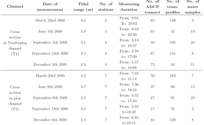
Table 1. Number of ADCP transects, transmissometer proles and water samples collected during measurement surveys at cross sections T1 and T2 under the PROMORPH project.
Channel Date of
measurement Tidal range (m) No. of stations Measuring duration No. of ADCP transect No. of trans. proles No. of water samples
March 22nd 2000 4.0 4 From: 8:04
To: 20:02 65 126 5
Cross section in Norderpiep
channel (T1)
June 5th 2000 3.8 4 From: 9:23
to: 20:59 61 32 14
September 5th 2000 3.1 4 From: 4:13
to: 16:57 59 105 28
September 12th 2000 3.2 4 From: 4:59
to: 17:09 67 131 8
December 5th 2000 2.3 4 From: 5:57
to: 18:08 73 44 11
March 23rd 2000 4.2 7 From: 7:33
to: 21:14 50 163 7
Cross section in piep channel
(T2)
June 6th 2000 3.7 7 From: 7:36
to: 16:24 37 90 15
September 6th 2000 2.5 7 From: 4:32
to: 15:50 27 91 24
September 13th 2000 3.4 7 From: 5:32
to:10:38 17 55 5
December 6th 2000 2.4 7 From: 6:40
to:19:11 44 130 8
Table 2. Properties of the mud fraction.
Period Tidal range (m) No. of measuring stations Settling velocity (mm/s) Critical bed shear stress for sedimentation
(N/m2)
Critical bed shear
stress for erosion (N/m2)
Erosion parameter (kg/m2/s) Mar. 21-23,
2000 4.0 20 1.60 2.88 0.89 5.10e-004
June 5-6,
2000 3.7 23 2.00 3.24 1.00 4.70e-004
Sept. 5-6,
2000 3.2 23 1.60 3.02 0.79 5.70e-004
Sept. 12-13,
2000 3.0 21 1.76 3.12 0.88 5.20e-004
Dec. 5-6,
2000 2.3 20 1.30 2.90 0.65 1.57e-004
to the availability of long time data collection at the site.
The grain size map of the area was developed by Escobar (2007) [5]. He carried out intensive experiments and determined a functional relationship between ow characteristic and grain size distribution. Regarding the sediment properties, altogether, ve sediment fractions were used, of which, four describe
the non-cohesive sediments and one represents the mud fraction. The mud content and properties of the non-cohesive sediment fraction were those derived from sed-iment samples taken at several locations, as reported by Poerbandono and Mayerle (2005) [4]. Characteristics of the cohesive fractions, accounting for 75% of the sediment mixture, are listed in Table 2.
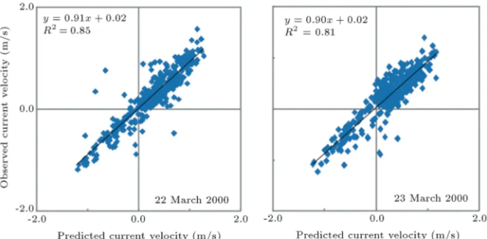
Figure 3. Measured versus predicted current velocity for cross sections T1 (left side) and T2 (right side).
waves under moderate winds, having velocities less than 11 m/s, is ignorable. In the simulations, there-fore, considering moderate conditions during all the campaigns, the eect of wind induced waves was withdrawn.
The hydrodynamic of the model was calibrated and validated by Palacio et al. (2005 ) [7], using collected ADCP data. They reported the mean ab-solute error of less than 0.2 m/s between computed and observed velocities at various cross-sections in the tidal channels. They also claimed that this value represents less than 20% of the tidally-averaged value, which can be considered an acceptable result for the hydrodynamic model. To show the relativity between the modeled and measured current velocity, Figure 3 is prepared. Measured velocities are presented on the vertical axis and modeled velocities are presented on the horizontal axis. The results for cross sections, T1 and T2, are presented in the left and right side, accordingly. The trend line for each graph is derived. Its equation and R-squared values are presented at the top of each graph. It can be seen that over 80% of the predicted current velocities are in good agreement with the measured ones.
To obtain SSC during the cruises of the PRO-MORPH project, the Niskin bottle, as a trap sampler, and the transmissometer, as an optical device, were employed. For collecting the SSC at dierent levels along the depth, the transmissometer, together with one CTD (Conductivity, Temperature and Depth) device, and one Niskin bottle sampler, were mounted on a frame. In each cruise, the frame was lowered at specied positions from the surface to near the bottom across each cross section. The CTD device in the frame provided the height at which the beam scatter data and samples are collected.
To convert the optical transmission data to SSC, the method described by Ohm (1985) [8] and Ricklefs (1989) [9] was employed. That is, those SSC de-termined from about 200 Niskin bottle samples were
plotted against the amount of transmission of light to derive a relationship. Through statistical analyses, Poerbandono (2003) [10] proposed Eq. (1) for this conversion:
c = (7A + 33)10 3; (1)
where, c is concentration of sediment, and A = L 1ln(I) is the attenuation coecient in which L
is the transmissometer path length in cm, and I is the optical transmission as a decimal fraction.
Using the RMAE method, Poerbandono (2003) [10] reported that the accuracy of optical measurements was about 30% on the basis of agreement with concentrations determined from physical samples. This low accuracy has been claimed to be due to the insucient sensitivity of the optical beam transmissometer with a path length of only 2 cm for detecting low concentrations [11].
These data made it possible to evaluate the results of the 3D model at every spatial position and temporal situation of the area under investigation. That is, the model was provided with the monitoring points at the same geographical positions of the points where measurements were carried out; monitoring points 1 to 4 at cross section T1, and 1 to 7 at cross section T2, in Figure 2. The model was executed for the same period as the measuring campaigns were carried out. The SSC data derived from the eld measurements were compared with those derived from the model.
4. Results and discussion
4.1. Evolution of the vertical proles of suspended sediment concentration
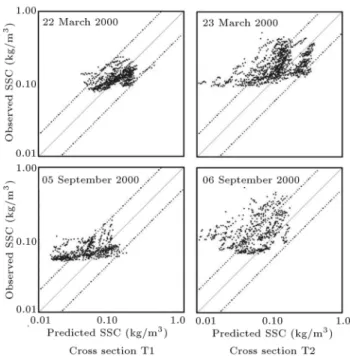
As a rst approach to verify the high quality of the model results, the SSC derived from the model were plotted against those derived from measurements. Figure 4 shows the scatter plot of the measured versus computed SSC, covering all simulated conditions for two cross sections, T1 and T2, during the neap and
Figure 4. SSC predicted by model versus SSC derived from the eld for cross-sections T1 and T2.
spring tide. The black dashed lines in the plots repre-sent a factor of 2 and the central solid line reprerepre-sents perfect agreement between the measured and predicted suspended sediment concentrations.
It can be seen that for the entire two periods of measurements, and at both cross sections, a high proportion of values are within a factor of two, which, according to Kleinhans and Van Rijn (2002) [12], is considered quite high quality for predicting SSC. However, in cross section T2, a considerable number of points are also located outside the factor of two, which shows relatively poor correlation between the model and eld data. The plots for other data sets mentioned in Table 1 showed the same pattern in both cross sections (see Rahbani (2011) [6]).
Two aspects that may aect the predictive ability of the sediment transport model, including: (a) the assessment of the eect of conditions specied along the open sea boundaries of the ow mode, and (b) the need to account for waves in the sediment transport simulations, were studied. Neither of these factors was found to be responsible (see Rahbani (2011) [6]).
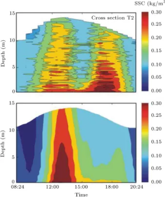
To verify the cause of dissimilarity observed at cross section T2, two comparing procedures were car-ried out. First, evolutions of the vertical prole of the SSC from the model for a monitoring point at the middle of each cross section were prepared and compared (Figure 5). Two successive high concentra-tions of suspended sediment, due to the ood and ebb phase, can be seen for cross section T1, which is usual when taking into account the semidiurnal nature of the area. However, this is not the case for cross section T2. According to the model results in cross section T2, a
Figure 5. The evolution of the vertical proles of SSC at middle point of cross sections T1 (the top graph) and T2 (the bottom graph).
high concentration of suspended sediment is achieved during the ood phase. During the ebb phase, however, an increase in SSC starts to shape at the bottom, which is terminated before its full development toward the surface.
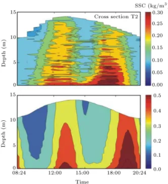
To nd out whether the evolution of the vertical prole of the SSC derived from eld data follows the same rule at cross section T2, a similar graph for the period when the measured data was available was prepared to compare with that derived from the model. That is, from 08:24 to 20:24 on March 23rd, 2000 (Figure 6). Unlike the model results, formation of two successive high concentrations of suspended sediment during the ood and ebb phase can be observed regard-ing eld data. It can also be seen that the two peaks are relatively close to each other (about a 4-hour interval between the two peaks) and that in the near bed region, the SSC remains high during the times between the two peaks, with values of about 0.25 kg/m3. This indicates
that the sediments suspended during the ood phase had insucient time to settle onto the bed completely. Thus, during the returning ebb, the current caused a further increase in the concentration of suspended sediment, that is, the explanation for the peak of SSC, because of the ebb current being higher than the peak, due to the ood current.
Referring to the graph for the model, as discussed, it seems that the established model is incapable of reproducing the peak SSC during the ebb phase at this cross section. The model deciency mentioned above
Figure 6. Evolution of the vertical proles of SSC from the eld data (the top graph) and the model results (the bottom graph) at the monitoring point at the middle of the cross section T2.
was observed in all monitoring points of cross section T2 (see Table 1).
From the results, it can be concluded that this incapability of the model might be the main reason for the deviations observed between the model and measured data at this particular cross section. The insucient supply of sediment during the ebb condition is responsible for this behaviour of the model. One of the parameters responsible for this behaviour is the grain size distribution of sediment particles introduced to the model. As reported by Escobar (2007) [5], the prepared map of grain size distribution was based on a limited number of measurements, specically on the tidal at areas. He pointed out the existence of some localized discrepancies between values in the map and actual values in the eld. He also mentioned that precise information regarding grain size distribution could improve the model results.
The other factor that might be responsible for the insucient supply of sediment is the use of a constant settling velocity for the channels and the tidal ats. Distribution of dierent grain size in the area is necessitated using dierent settling velocities. Analysis of laboratory and eld data has shown that the settling velocity of the ocs is related to the sediment concen-tration [13], the water depth [14], the ow velocity [15], and occulation and biological activities [16]. Thus, the settling velocity for tidal channels cannot be the
where band ceare bed shear stress and critical surface
erosion shear stress, respectively, Mer and is the mass
erosion rate constant.
The diculties inherent in measuring this pa-rameter in the eld have prevented the preparation of a map of the distribution of CBSSE for the area. Therefore, this parameter is dened to the model as a single value for the whole area under investigation.
A combination of the above mentioned factors are involved in the deciency observed in the performance of the model, specically, at cross section T2.
4.2. Snapshots of suspended sediment concentrations in cross sections
As another eort, the patterns of SSC distribution along cross sections T1 and T2 predicted by the model were prepared and compared with those derived from the measured data. That is, the snapshot of the distribution of SSC for cross sections T1 and T2 during dierent phases of a tidal cycle were prepared for both model results and eld data.
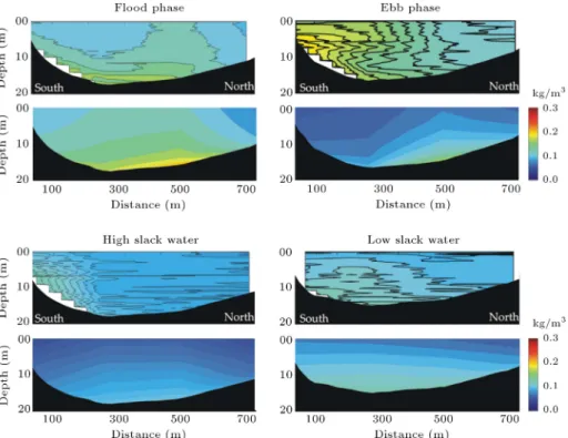
Figures 7 and 8 show snapshots of times of ood, high slack water, ebb, and low slack water for cross sections T1 and T2, respectively. The top snapshot for each pair is from the eld data and the one below is from the model results.
As expected, the snapshots in Figure 7 show good agreement between the modeled and measured SSC during dierent tidal phases at cross section T1. The concentration of suspended sediment is quite low in this cross section, and never exceeds 0.2 kg/m3during a full
tidal cycle.
According to Figure 8, however, the distribution of SSC derived from the model and measured data are not in good agreement for all tidal phases. It can be seen that during the ood phase, both the model and the eld plots show the same pattern of distribution of SSC across the cross section. That is, the concentration, which is high in the bed to the middle layers of the southern bank region, decreases gradually towards the surface and the northern bank region. The SSC values are higher for the model plot.
At the following high slack water, the model plot shows high SSC at the deep region of the cross section
Figure 7. Snapshots of SSC distribution for ood, high slack water, ebb, and low slack water phase at cross-section T1. The top snapshots of each pair represent eld data and the bottom ones show model results.
near the northern bank, but the eld plot shows high SSC in the shallow region of the cross section near the southern bank. This plot also shows that the SSC decreases abruptly toward the surface and the northern
bank region, with the exception of an area of a high concentration in the middle of the cross section.
During the following ebb phase, the eld plot shows the same pattern as that during the ood phase,
Figure 8. Snapshots of SSC distribution for ood, high slack water, ebb, and low slack water phase at cross-section T2. The top snapshots of each pair represent eld data and the bottom ones show model results.
high slack water. The reason for the low values of SSC during the ebb phase of this cross section was discussed in detail in Section 4.1.
The concentration of suspended sediment at this cross section is relatively high, especially in the southern bank of the section, with the values exceeding up to 0.35 kg/m3 during ebb and ood
phases.
4.3. The eect of critical bed shear stress It is mentioned in Section 4.1 that the reason for considering the constant erosion rate in the area was the lack of eld data. It is, however, obvious that the Critical Bed Shear Stress for Erosion (CBSSE), thus, the erosion rate, is not the same everywhere in the area, specically, not the same on the tidal at and in the tidal channel. As a trial, a map has been prepared for the CBSSE, with the values for the tidal at area being 50% less than those of the tidal channel. That is, to allow more sediment to be suspended and transported by the ebb current from the tidal at area. The map is introduced to the model instead of a plain value of erosion rate. Using this map, the model was executed. The result, which is presented in Figure 9, shows successive peaks of SSC due to the ebb current as well as the ood current. It can also be seen that the peak of SSC during the ebb phase is higher than that during the ood phase, which is the case for the eld data. It should, however, be mentioned that the usage of this map of CBSSE has caused considerable increase in the SSC values for the whole period of tidal condition. That is, the concentration of suspended sediment is elevated to about 0.5 kg/m3. It should
be emphasized that the map of CBSSE was prepared by the author, executing several trials. It is not made on the basis of eld measurements.
The output of this model is also used to prepare snapshot plots of the cross section with the revised values for CBSSE (Figure 10). Referring to this gure, successive performance of the model was achieved during the ebb phase. That is, the peak of SSC inuenced by the ebb current is reproduced by the model. However, as seen, overprediction is imposed
Figure 9. Evolution of the vertical proles of SSC from the eld data (the top graph) and from the model results using low value of critical bed shear stress for erosion for the tidal at and high value for tidal channel (the bottom graph).
onto SSC values computed by the model all over the cross section and for all tidal stages. This was also the case in Figure 9.
5. Conclusion
To evaluate the ability of the Delft3D model to predict Suspended Sediment Concentration (SSC) of the Piep tidal channel system, modeled data were compared with eld data using two dierent experiments, in-cluding evolution of the vertical proles of SSC in a monitoring point at the middle of the cross sections, and the snapshots of SSC in the cross sections.
In comparative analyses of the SSC proles de-rived from the model with those dede-rived from the eld, some dissimilarities was observed relating to the ebb current and low slack water of cross sections T2. That is, the model could not simulate the peak SSC during the ebb current at this cross section.
The insucient supply of sediment from the tidal at area on the eastern side of this cross section was found to be responsible for this behaviour of the model. In other words, the modelled tidal at areas do not supply sucient sediment during the ebb current. Several parameters and/or factors have been mentioned as being responsible for this insucient supply of sediment, including the grain size map introduced to the model, the usage of one plain settling velocity for the whole area, and the usage of a constant value of erosion rate for the area.
Figure 10. Snapshots of SSC distribution for ood, high slack water, ebb, and low slack water phase at cross-section T2. The top snapshots of each pair represent eld data and the bottom ones show model results (employed revised CBSSE).
According to Wiberg (2012) [17], sediment sus-pension in Delft3D, for a given bed shear stress, is controlled primarily by settling velocity and an erosion rate parameter. Critical shear stress must also be specied, but it is not allowed to vary with depth or mass eroded. The paper also mentioned that SSC in the model calculations is more sensitive to the erosion rate parameter than to settling velocity.
It is also reported by Gourgue et al. (2013) [18] that the settling velocity of suspended sediments is inuenced by occulation. The important factors governing this process include the SSC itself, turbu-lence, shear stress, salinity, biological activity and some physicochemical properties. It, therefore, cannot be considered the same for dierent spatial conditions.
It should also be emphasized that the hydro-dynamic of the model itself can be responsible for some deciency observed in the SSC predicted by the model. That is, even though the hydrodynamic of the model was veried by as good as 80%, it can still cause part of the shortcomings observed in the model results.
The input of dierent values of the Critical Bed Shear Stress for Erosion (CBSSE) for the tidal at areas and the tidal channel eastward of cross section T2 did improve the model results.
The necessity for the production of a CBSSE map on the basis of eld data and model simulations is, therefore, suggested for improvement of the model results.
In short, it can be concluded that the developed
model is suciently accurate to provide values of the suspended material concentration comparable with those of eld data to a certain extent. It, however, should be emphasized that, in order to achieve reliable results, precise eld measurements all over the area, with the aim of estimating critical bed shear stress for erosion, need to be carried out.
Acknowledgments
The author would like to thank Professor Dr. Roberto Mayerle for his supervision and full support during her PhD research. He challenged her to produce her best work, and this paper is part of that research, which has been carried out in the Coastal Research Laboratory of Kiel University, Germany.
References
1. Souza, L.B.S., Schulz, H.E., Villela, S.M., Gulliver, J.S. and Souza, L.B.S. \Experimental study and nu-merical simulation of sediment transport in a shallow reservoir", Journal of Applied Fluid Mechanics, 3.2, pp. 9-21 (2010).
2. Mayerle, R. and Zielke, W. \PROMORPH - pre-dictions of medium-scale morphodyanimcs: Project overview and executive summary", Die Kuste, Heft, 69, pp. 1-24 (2005).
3. Nguyen, D., Etri, T., Runte, K. H. and Mayerle, R. \Morphodynamic modeling of the medium-term mi-gration of a tidal channel using process-based model",
7. Palacio, C., Mayerle, R., Toro, M. and Jimenez, N. \Modelling of ow in a tidal at area in the south-eastern German Bight", Die Kuste, Heft, 69, pp. 141-174 (2005).
8. Ohm, K. \Optical measurements for determination of suspended material transport\, [in German] (Optis-che Messungen zur Bestimmung von Schwebstotrans-porten), Die Kuste, Heide/Holstein, 42, pp. 227-236 (1985).
9. Ricklefs, C. \On sedimentology and hydrography of the Eider- Aster", [in German] (Zur Sedimentologie und Hydrographie des Eider- Astuars), Berichte Nr. 35 - Geologisch Palaontologisches Institut, Christian-Albrechts-Universitat, Kiel (1989).
10. Poerbandono \Sediment transport measurement and modeling in the Meldorf Bight tidal channels, German north sea coast", Ph.D. Thesis, Coastal Research Laboratory, University of Kiel, Germany, 151 pp. (2003).
11. Poerbandono and Mayerle, R. \Eectiveness of acous-tic proling for estimating the concentration of sus-pended material, die Kuste, Heft 69, pp. 393-408 (2005).
12. Kleinhans, M.G. and Van Rijn, L.C. \Stochastic prediction of sediment transport in sand-gravel bed rivers", Journal of Hydrological Engineering, 128(4), pp. 412- 425 (2002).
ence B.V., editor, Proceedings in Marine, 5, P.O. Box 211, 1000 AE Amsterdam, The Netherlands (2002).
17. Wiberg, P., Erodibility and Stability of Tidal Flats: Characterization and Prediction, G.N.: N00014-07-1-0926, University of Virginia (2012).
18. Gourgue, O., Baeyens, W., Chen, M.S., de Brauwere, A., de Brye, B., Deleersnijder, E. and Legat, V. \A depth-averaged two-dimensional sediment transport model for environmental studies in the Scheldt Estuary and tidal river network." Journal of Marine Systems, 128, pp. 27-39 (2013).
Biography
Maryam Rahbani was born in Shiraz, Iran. She obtained her BS degree in Mechanical Engineering from Sharif University of Technology, Tehran, Iran, in 1991, and her MS degree in Physical Oceanography from the University of Chamran, Iran, in 1999 (the intrusion of Anzali wetlands into the Caspian Sea, using numerical modelling). She moved to Germany in 2004 to pursue her PhD degree (thesis Entitled \Numerical modelling of the coastal processes in Dithmarschen Bight, in-corporating eld data") using the Delft3D model, a well-known software in oceanographic sciences. She is currently Assistant Professor at the University of Hormozgan, Iran.