Video Quality Driven Buffer Sizing via Frame Drops

University of Pennsylvania

ScholarlyCommons

Departmental Papers (CIS)

Department of Computer & Information Science

8-2011

Video Quality Driven Buffer Sizing via Frame

Drops

Deepak Gangadharan

National University of Singapore, [email protected]

Linh T.X. Phan

University of Pennsylvania, [email protected]

Samarjit Chakraborty

TU Munich, Germany, [email protected]

Roger Zimmermann

National University of Singapore, [email protected]

Insup Lee

University of Pennsylvania, [email protected]

Follow this and additional works at:

http://repository.upenn.edu/cis_papers

Part of the

Computer Sciences Commons

17th IEEE International Conference on Embedded and Real-Time Computing Systems and Applications (RTCSA), Toyama, Japan, Aug 2011. This paper is posted at ScholarlyCommons.http://repository.upenn.edu/cis_papers/473

For more information, please [email protected].

Recommended Citation

Deepak Gangadharan, Linh T.X. Phan, Samarjit Chakraborty, Roger Zimmermann, and Insup Lee, "Video Quality Driven Buffer Sizing via Frame Drops",17th IEEE International Conference on Embedded and Real-Time Computing Systems and Applications (RTCSA 2011)1, 319-328. August 2011.http://dx.doi.org/10.1109/RTCSA.2011.49

Video Quality Driven Buffer Sizing via Frame Drops

We study the impact of video frame drops in buffer constrained multiprocessor system-on-chip (MPSoC)

platforms. Since on-chip buffer memory occupies a significant amount of silicon area, accurate buffer sizing

has attracted a lot of research interest lately. However, all previous work studied this problem with the

underlying assumption that no video frame drops can be tolerated. In reality, multimedia applications can

often tolerate some frame drops without significantly deteriorating their output quality. Although system

simulations can be used to perform video quality driven buffer sizing, they are time consuming. In this paper,

we first demonstrate a dual-buffer management scheme to drop only the less significant frames. Based on this

scheme, we then propose a formal framework to evaluate the buffer size vs. video quality trade-offs, which in

turn will help a system designer to perform quality driven buffer sizing. In particular, we mathematically

characterize the maximum numbers of frame drops for various buffer sizes and evaluate how they affect the

worst-case PSNR value of the decoded video. We evaluate our proposed framework with an MPEG-2 decoder

and compare the obtained results with that of a cycle-accurate simulator. Our evaluations show that for an

acceptable quality of 30 dB, it is possible to reduce the buffer size by upto 28.6% which amounts to 25.88

megabits.

Disciplines

Computer Sciences | Physical Sciences and Mathematics

Comments

17th IEEE International Conference on Embedded and Real-Time Computing Systems and Applications

(RTCSA), Toyama, Japan, Aug 2011.

Video Quality Driven Buffer Sizing via Frame Drops

Deepak Gangadharan

, Linh T.X. Phan

, Samarjit Chakraborty

, Roger Zimmermann

, Insup Lee

_{National University of Singapore,}

_{University of Pennsylvania, USA,}

_{TU Munich, Germany}

E-mail:{gdeepak,rogerz}@comp.nus.edu.sg,

{linhphan,lee}@cis.upenn.edu, [email protected]

buffer-constrained multiprocessor system-on-chip (MPSoC) platforms. Since on-chip buffer memory occupies a significant amount of silicon area, accurate buffer sizing has attracted a lot of research interest lately. However, all previous work studied this problem with the underlying assumption that no video frame drops can be tolerated. In reality, multimedia applications can often tolerate some frame drops without significantly deteriorating their output quality. Although system simulations can be used to perform video quality driven buffer sizing, they are time consuming. In this paper, we first demonstrate a dual-buffer management scheme to drop only the less significant frames. Based on this scheme, we then propose a formal framework to evaluate the buffer size vs. video quality trade-offs, which in turn will help a system designer to perform quality driven buffer sizing. In particular, we mathematically characterize the maximum numbers of frame drops for various buffer sizes and evaluate how they affect the worst-case PSNR value of the decoded video. We evaluate our proposed framework with an MPEG-2 decoder and compare the obtained results with that of a cycle-accurate simulator. Our evaluations show that for an acceptable quality of 30 dB, it is possible to reduce the buffer size by upto 28.6% which amounts to 25.88 megabits.

I. INTRODUCTION A. Motivation

Decoding video content on video playback devices requires significant amount of on-chip buffer resources for storing the incoming/partially processed frames. Therefore, accurate buffer sizing in multimedia MPSoC platforms has attracted lot of research attention. All the prior works in buffer sizing (e.g., [11], [9] and [15]) did not tolerate video quality loss at the output, i.e., they did not allow frame drops. On the other hand, there have been works on frame dropping strategies ([7] and [17]) to maximize video quality output in the presence of buffer constraints. However, there has been no work on quality driven buffer sizing using a frame dropping strategy. Such a strategy would be very useful as it is a well known fact that multimedia applications can tolerate some quality loss without deteriorating the video perception.

In this paper, we propose a formal framework to explore the buffer size vs. video quality trade-offs, which can help a system designer to perform quality driven buffer sizing. Although these trade-offs can be explored using system simu-lations, simulation-based techniques are time consuming. The concepts discussed here, however, can be applied in the context of network- on-chip architectures where buffer size can be traded off against some quality parameter by dropping the less important data. In general, it is applicable to all such scenarios where losing some low priority data helps in saving buffer resources while still maintaining a good content quality. Therefore, it is important to recognize the least important data

I and P frames

B_inf

Bfin

PE

to subsequent PE

…

B frames

Splitter

Incoming frames

Frame drops

P Frame ordering information

0 100 200 300 400 30

35 40 45

Frame Interval

(W

o

rs

t

C

a

s

e

)

P

S

N

R

(

in

d

B

)

Bm

a

x

=

3

0

Bm

a

x

=

9

0

Bm

ax

=

1

5

0

Acceptable quality

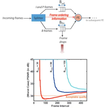
Fig. 1. Dual buffer management scheme with drops in less significant frames and buffer size vs. video quality trade-off results for a benchmark MPEG-2 videosusi080 ([12]).

in the target application. As our framework bounds the quality degradation, the video quality does not deteriorate too much. In MPEG-2/MPEG-4 video streams, there are typically three

types of frames, namely,I frame(Intra coded),P frame

(Pre-dicted) and B frame(Bidirectionally predicted). I frames are

intra coded frames and are not dependent on other frames in the video stream for decoding. Decoding a P frame requires the previous I or P frame as the reference frame. Finally, decoding a B frame requires two reference frames, namely, a forward reference frame (I/P frame) and a backward reference frame (I/P frame). It is clear from this organization of frames that B frame drops result in lesser amount of quality degradation in comparison to the I and P frame drops. Therefore, in MPEG-2/MPEG-4 decoder applications mapped onto MPSoC platforms, B frame drops can be used to trade-off quality for buffer size. This selective dropping of frames requires a special scheme to differentiate among frames.

In our approach, a simple dual buffer management scheme is used in order to drop only the less significant frames (B frames). This scheme is shown in Fig. 1. The incoming multimedia stream is split into two distinct streams: the first consists of the less significant frames (B frames) and the sec-ond consists of the more significant ones (I/P frames). These two streams are fed to two distinct buffers. This partitioning

will be explained in detail in Section III. The processing element (PE) needs to be given a side information conveying the order in which the frames are to be processed (shown as the dotted line from the splitter to the PE in Fig. 1). In the setup shown in Fig. 1, drops occur only for B frames and the size of the associated buffer can be traded off with video quality. This trade-off (shown in Fig. 1) is obtained using a

well known video benchmarksusi 080 ([12]). In multimedia

literature ([19]), 30 dB is considered to be an acceptable output video quality (shown as the horizontal line in the trade-off graph in Fig. 1). From Fig. 1, it can be observed that we give quality variations for three different buffer sizes over frame intervals. We define frame interval below.

Definition 1: (Frame Interval). For a given video clip, a

frame intervalF is defined as a window of anyF consecutive

frames.

The worst case quality value for a frame interval F is the

minimum quality obtained over any F consecutive frames

across the clip. From Fig. 1, it can be observed that if a

maximum buffer size (Bmax) of 30 frames is chosen, then the

quality values (in dB) fall below the threshold value of 30 dB for certain frame intervals from 80 to 260. If the target quality constraint is to satisfy the 30 dB value for all frame intervals,

thenBmax=30 frames will not be sufficient. However, if the

target quality constraint is that the threshold value of 30 dB should be satisfied for any frame interval greater than 300,

then Bmax= 30 frames will be a good choice as the buffer

size. We denote buffer sizes in number of frames in the rest of the paper because video frames consist of variable number of bits. However, we give an estimate of the minimum buffer savings in megabits (Mbs).

B. Our Contributions

To the best of our knowledge, this is the first attempt at studying the influence of buffer sizing on worst case quality deterioration using a formal framework. There are two interlinked parts constituting our framework. For a given video clip, we perform the following operations.

1) Firstly, we derive the maximum number of frame drops (in any frame interval) for any given buffer size using a Network Calculus ([2]) based mathematical framework. 2) Secondly, we propose a novel method to compute worst case quality values for video clips. This is further used in conjunction with the maximum number of frame drops derived in the first part to find the worst case quality values for various buffer sizes.

A system designer does buffer sizing for an extensive library (covering all possible scenarios) of video clips, whereby sufficient buffer size is chosen so that a quality constraint is satisfied by all the clips in the library. Our framework can be used in this context. The information obtained from buffer size vs. quality trade-off curves for each clip can be used to determine the optimal buffer size for the entire library. C. Related Work

On-chip buffers take up a lot of chip silicon area. This is evident from [6], in which experiments clearly show the

enormous amounts of silicon area increase due to the increase in FIFO size in the router. In [18], this same concern is demonstrated in the context of on-chip network design for multimedia applications. However, the authors do not drop any incoming packet from the buffer thereby giving importance to maximum application quality. A buffer sizing algorithm has been discussed in the context of networks on chip [3], where the authors are concerned about the reduction of buffers in network interfaces. There are various objective functions that are considered while choosing the appropriate buffer size. A buffer allocation strategy is proposed in [6] in order to increase the overall performance in the context of a networks-on-chip router design. In [14], an appropriate buffer size is chosen that gives the best power/performance figure.

Buffer dimensioning is an important aspect of designing media players. In the past, there has been lot of work in this area where several design factors have been taken into consideration while choosing the appropriate buffer size. Most of this work concentrated on studying the playout buffer vs. quality of service (QoS) tradeoffs. In [8], the authors discussed an optimal allocation of playout buffer size such that the playout delay is minimized for a given probability of underflow or a given QoS. Similarly, in [4], the buffer vs. QoS tradeoff is studied for multimedia streaming in a wireless sce-nario using a dynamic programming framework. A combined optimal transmission bandwidth and optimal buffer capacity is considered to support video-on-demand services [20]. Here, playout buffer overflow and underflow are not tolerated. There are also some other prior works which have not tolerated any loss as a result of buffer overflow and underflow ([10], [11], [9] and [15]). However, none of these works have considered the tradeoff between buffer and video quality by allowing some buffer overflows (i.e., with constrained buffer). Here, video quality is not the end-to-end QoS, but the distortion in the received frames.

There are various frame dropping strategies that have been discussed in literature that try to maximize the video quality ([7] and [17]). Invariably, all these strategies use a prioritiza-tion scheme to drop the frames in a quality aware manner such that the quality deterioration is minimized. In [7], frame size is used to prioritize the frames before dropping. In this approach, frames with larger size are dropped later and frames with smaller size are dropped first. A distortion matrix is introduced in [17] to compute the priority of frame dropping based on the distortion that frame suffers if lost. As we drop only the B frames in this paper, we consider the drop oldest policy

during a buffer overflow. Similar schemes likeDrop Newest,

Drop RandomandDrop Allare also discussed in [16].

D. Organization of the Paper

In the next section, we give an overview of our analytical framework. Section III discusses the process of partitioning the arrival and service curves in order to analyze the dropping of only certain frames, i.e., B frames. In Section IV, we present the theory behind the calculation of maximum number of frame drops for any frame interval. Section V presents the analytical framework to derive the worst-case quality curve

from frame drop bounds. Section VI discussed a case study of MPEG-2 decoder application. In Section VII, we present the concluding remarks.

II. FRAMEWORKOVERVIEW

This section presents an overview of our mathematical framework to study the influence of frame drops on the peak signal to noise ratio (PSNR) of the decoded video under buffer constraints. We use the arrival curves and service curves from the Network Calculus to model the data streams and the service given by the resources, respectively, as they can model any arbitrary stream arrival pattern and any arbitrary resource service pattern. In addition, they can easily capture the data size variability and the processing variability exhibited in the multimedia setting we consider here. Before describing our framework, we introduce the underlying MPSoC platform.

Platform Description: In this work, we find the buffer size vs. worst case quality trade-off for a video clip on a buffer constrained MPSoC architecture as shown in Fig. 2. The terms explained in the problem definition are marked appropriately alongside the architecture. The architecture

consists of two PEs, PE1 and PE2, each with its own offered

service curves shown above them. Each PE is mapped with a set of tasks from the target decoder application. The PEs

also each have a buffer in front of them, shown as B1 and

B2, with maximum capacity of B1max and B2max (quantified in number of frames), respectively. As the buffer sizes are not always adequate, frame drops may occur, which are

characterized as αu

drop1(∆) and αdropu 2(∆). αdropu 1(∆) and

αu

drop2(∆) give the upper bounds on the number of frames

dropped in any time interval of length ∆, where ∆ ≥0.

Although only a single buffer is shown in front of each PE, each buffer internally has two parts - one part where some of the least significant contents (B frames) are dropped and the second part where adequate buffer size is provided and the significant contents (I/P frames) are not dropped. The frame drops occur in the droppable buffer section and its drop bounds are derived by our framework. Before getting into the details of our framework, we first define some terminology. Definition 2: (Arrival Curve). For a video clip, let a(t) denote the number of frames that arrive in time interval[0,t). Then, the video clip is said to be bounded by the arrival curve

α= [αu_,αl_{] iff for all arrival patternsa(t):}

αl_{(∆)≤a(t+∆)−a(t)≤α}u_{(∆) (1)} for all ∆≥0. In other words, αu_{(∆) and α}l_{(∆) give the} maximum and minimum number of frames that can arrive over any interval of length ∆across the length of the video clip.

input stream

B1

α

β1 B2

to playout buffer

PE₁

αdrop2 u

αdrop1 u

β₂

PE2

Fig. 2. MPSoC setup with buffer constraints and frame drops

B

PE

drop u input

stream

drop

u

Q

u

q

u

Frame interval

Frame interval

Frame inter

val No. of frames

dropped

(No. of frames dropped)

(worst case quality)

B

PE

drop u input

stream

drop

u

Frame interval (No. of frames dropped) dropped)

(worst case quality)

Q

u

q

u

Frame interval

Frame inter

val No. of framesof fram es dropped dropped

(worst case quality)

(worst case quality)

Drop bound calculation Quality bound calculation

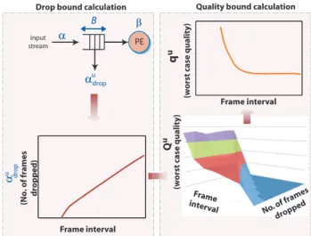
Fig. 3. Overview of the Analytical Framework

Definition 3: (Service Curve). Letc(t)denote the number of frames processed by a task mapped onto a processor in time interval[0,t). Then, the service curveβ= [βu_,βl_{]is a service} curve of the processor iff for all service patternsc(t):

βl_{(∆)≤c(t+∆)−c(t)≤β}u_{(∆) (2)} for all ∆≥0. In other words, βu_{(∆) and β}l_{(∆) denote the} upper and lower bounds on the number of frames processed over any interval of time∆across the length of the clip.

Problem Definition: Given the arrival curve [αu_,αl_{] of the} video clip that is to be decoded on a decoder application mapped onto a MPSoC platform, the service curve [βu_,βl_], we analytically explore the trade-off between buffer resource Bmax (measured in number of frames) and the worst case quality (quantified in terms of PSNR) of the decoded video.

Once this trade-off is explored for all the clips in the library, the system designer can appropriately choose the minimal buffer resource required to satisfy an acceptable quality constraint. The overall analytical framework consists

of two stages as shown in Fig. 3, namely the Drop bound

calculation stage and the Quality bound calculation stage. These two stages are described briefly next.

Drop bound calculation: The first stage formally derives the

worst case frame drop boundαu

drop for the droppable part of the buffer, with size Bmax. This analysis is based on concepts from network calculus. Specifically, it computes the bounds on the number of frames that are processed in an incoming stream when the arrival curves[αu_,αl_{], service curves[β}u_,βl_] and buffer sizeBmaxfor a single PE are given. Our computation is based on the idea of a virtual processor controlling the admission of frames into the buffer such that the buffer effectively acts as one with no drops, i.e., once an appropriate number of frames are dropped from the stream, the finite and constrained buffer will never overflow, thereby emulating an infinite buffer. We also compute the bounds on the service offered by the virtual processor to the incoming stream. This can be used to compute the worst case bound on the number of frame drops in any interval of time. However, we convert

the time interval based computation of frame drop bounds into

frame interval based boundsαu

dropF(F), whereF is the frame interval window and 1≤F≤Ftotal. Here, αdropFu (F) is the upper bound on the number of frames dropped in a window of

F consecutive frames andF_total is the total number of frames

in the clip. The detailed formulation will be shown in Section IV.

The useful feature of this stage is that it allows the analysis of multiple PEs in pipeline with buffer constraints to be done compositionally. In other words, one can compute the bounds on the arrival curve to the next stage. The computed arrival curve can then be used to derive the frame drop bounds in the next stage. These frame drop bounds computed at various stages (with constrained buffer resources) can be finally summed up to obtain the overall bound on the frame drops.

Quality Bound Calculation: Once the frame drop bounds are known, we compute a frame interval based worst-case bound on quality in terms of PSNR. Towards this, a parameter called the worst-case quality surface, denoted by Qu, is constructed for each video clip. Qu is defined as below.

Definition 4: Worst-case quality surface (Qu_{). For any} frame intervalF, the worst-case quality surfaceQu_{(f,F), for} all 0≤f≤F, is the worst-case quality of the video if f frames

are dropped in any window ofF consecutive frames.

All dropped frames are replaced by immediately preceding

and successfully processed frames calledconcealment frames.

The amount of quality loss depends on the mean square error (MSE) between the dropped and concealment frames. The resultant quality is measured in terms of PSNR, which in turn depends on the MSE between the dropped and concealment frames. We find all possible concealment frames for a dropped video and analyze which concealment frame results in maximum error or worst quality degradation. Bmaxvs. quality trade-off: The final goal of the framework is to explore the trade-off between the maximum buffer capacity

Bmax and the quality for each video clip in the library. Once

this trade-off is available for all the clips in the library, the system designer can take a well-informed decision on the appropriate buffer size. In order to derive this trade-off, we

use the frame drop bound αu

dropF and map it into the worst case quality surfaceQu(f,F)where f is replaced by the value

αu

dropF. Therefore, the quality bound calculation is a mapping from a three dimensional (3D) space to a two dimensional (2D) space shown as

qu(F) =Qu(αu

drop(F),F) (3)

where qu(F) is the worst-case quality bound for the video

clip. This mapping is shown in Fig. 3, where the frame drop bounds are shown at the bottom left hand side and the worst-case quality space is shown on the bottom right hand side. The final worst-case quality bound for a video clip is shown in the top right hand side of Fig. 3.

III. PARTITIONING ARRIVAL AND SERVICE CURVES In this paper, we study the effect of frame drops in the context of a video clip being processed by the associated

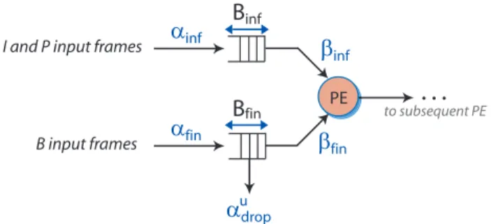
decoder application. As we are more interested in studying the effect of frame drops on quality degradation, we intend to analyze the drop of those frames that least affect the quality degradation. It has been observed in MPEG-2 or MPEG-4 decoders that B frames are generally the least significant when compared to I and P frames as the loss of B frames results in least quality degradation when compared to I and P frames. Moreover, many video clips are encoded with a IPBBPBBP... frame pattern, where a large percentage of B frames exist. Therefore, we analyze the effect of only the B-frame drops. If there are videos encoded without B frames, then P frames can be dropped. In this case, the framework will remain the same. Consequently, the system model for the platform architecture consists of two kinds of buffers in front of each PE depending on whether B frame drops are allowed or not. This is shown in Fig. 4. If B frame drop is allowed, then we have a finite buffer called the B frame buffer (Bf in)) and another finite buffer called the IP frame buffer (Bin f)) that does not have any drop. The buffer size required for an IP frame buffer can be computed using conventional Network Calculus technique ([2]).

The existence of two buffers makes it necessary to partition the arrival curves and service offered to the two sets of frames. As illustrated in Fig. 4, the original arrival curves of the input stream are partitioned into αin f = [α_{in f}u ,α_{in f}l ] and αf in= [αuf in,αlf in], which correspond to the arrival curves of the I and P frames together and of the B frames, respectively. Similarly, the service curves offered by the PE are partitioned intoβin f = [βin fu ,βin fl ]andβf in= [βuf in,βlf in], which correspond to the service curves offered to the I and P frames and to the B frames, respectively. As the I and P frames share the

same buffer Bin f with no frame drops, their buffer size can

be computed directly from αin f andβin f using the technique in [2]. On the other hand, the B frames can be dropped; their drop bound (αu

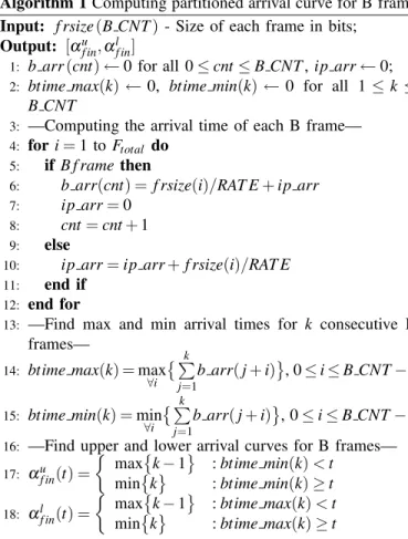
drop) can be computed usingαf in,βf inandBf in. The algorithm to compute the partitioned arrival curve for B frames is shown as Algorithm.1. The arrival curves for I and P frames can also be computed in the same manner. However, due to the existence of partitioned arrival curves and two buffers now, the PE needs to be given information about what is the order in which the frames are processed. This is generally the order in which the frames are encoded and sent out in a video stream.

In Algorithm 1, we compute the arrival curves [αu

f in,αlf in] for the B frames. Lines 4-12 compute the arrival times of each B frame (denoted byb arr) in the video clip.FtotalandB CNT

I and P input frames

B

B

α

to subsequent PE

…

B input frames

β

α

α

_β

fin

Algorithm 1Computing partitioned arrival curve for B frame

Input: f rsize(B CNT)- Size of each frame in bits;

Output: [αu f in,αlf in]

1: b arr(cnt)←0 for all 0≤cnt≤B CNT,ip arr←0; 2: btime max(k)←0, btime min(k)←0 for all 1≤k≤

B CNT

3: —Computing the arrival time of each B frame—

4: fori=1 to Ftotal do 5: ifB f ramethen

6: b arr(cnt) = f rsize(i)/RAT E+ip arr 7: ip arr=0

8: cnt=cnt+1

9: else

10: ip arr=ip arr+f rsize(i)/RAT E

11: end if

12: end for

13: —Find max and min arrival times for k consecutive B

frames—

14: btime max(k) =max

∀i

Pk

j=1

b arr(j+i) , 0≤i≤B CNT−k

15: btime min(k) =min

∀i

Pk

j=1

b arr(j+i) , 0≤i≤B CNT−k

16: —Find upper and lower arrival curves for B frames—

17: αu_{f in}(t) =

maxk−1 :btime min(k)<t mink :btime min(k)≥t 18: αl_{f in}(t) =

maxk−1 :btime max(k)<t

min

k :btime max(k)≥t

are the total number of frames and B frames, respectively, in the video clip. The input bit rate of the video clip is denoted by RAT E. We then find the maximum and minimum arrival times forkconsecutive B frames. This is shown in lines 14-15. Finally, the arrival curves are computed as in lines 17-18. The upper bound on the B frame arrival curve is obtained from the

minimum arrival time required for kconsecutive frames such

that they satisfy the condition in line 17. Similarly, the lower bound of B frame arrival curve is determined by the maximum arrival time required fork consecutive frames.

The service curves [βu

f in,βlf in] for B frames are also com-puted as the arrival curves have been comcom-puted. The only difference here is that instead of the arrival times of B frames, we compute the time required for the execution of the tasks

mapped on the PE for each B frame, i.e., b arr is changed

to execution time. Execution time also depends upon the frequency allocated to the PE. Subsequently, we compute

the maximum and minimum execution time required for k

consecutive B frames. Finally, we compute the service curves in a similar manner as we did for arrival curves. The arrival and service curves used in the following sections are the partitioned arrival and service curves for B frames presented here.

IV. BOUNDS ON DROPPED FRAMES

In this section, we present a method for computing bounds on the number of frames that are dropped due to an overflow at a buffer. We first present the modeling idea and the basic concepts, and then present the details of how drop bounds

can be obtained.

A single buffer case. Consider an input stream that is processed by a single processing element (PE). Suppose the input buffer that stores the incoming frames of the stream

before being processed by the PE, has a finite capacity ofB

frames. If the buffer is full when a frame arrives, the oldest frame at the head of the buffer will be dropped and the newly arrived frame will be enqueued at the end of the buffer. We are interested in the maximum bounds on the frames that can be dropped over any interval of a given length. The system architecture is shown in the top part of Figure 5. In the figure, a1(t) denotes the input arrival pattern of the frame, i.e., a1(t) gives the number of frames that arrive over the time interval(0,t]. Similarly,a3(t)gives the number of output frames corresponding to a1(t), respectively, over the interval (0,t].

To model the buffer refresh at the input buffer, we use a virtual processorPv that serves as an admission controller, as shown in the bottom part of Figure 5. The virtual processor Pv splits the input stream a1(t)into two disjoint streams: the former, a2(t), contains the frames that will go through the system, and the latter,a0₂(t), contains the frames that will be dropped, such that there are no overflows at the buffer.

B

PE

β

…

input stream

finite buffer

PE

β

…

input stream

infinite

P

virtual processor

a₁(t) a₂(t) a₃(t)

a

′

dropped frames

a₁(t) a₃(t)

drop modeling

Fig. 5. Modeling systems with drop due to buffer overflow.

Based on this transformed system, we give the relationship between a1(t) and a2(t), and the bounds on a3(t), stated

by Lemma 4.1 and 4.2. The (min,+) convolution ⊗ and

deconvolutionoperators are defined as:

f⊗g(t) = inff(s) +g(t−s)| 0≤s≤t , fg(t) = supf(t+u)−g(u)|u≥0 .

Similarly, the (max,+) convolution ⊗ and deconvolution

operators are defined as: f⊗g

(t) =sup

f(s) +g(t−s) | 0≤s≤t , fg(t) =inf

f(t+u)−g(u) | u≥0 .

In what follows, g∗ denotes the sub-additive closure of g,

defined byg∗=mingn|n≥0 , whereg0(0) =0 andg0(t) = +∞ for all t >0, and gn+1=gn ⊗ g for all n∈N_, n≥0. Further,I denotes the linear idempotent operator, i.e.,

Ia1(x)(t) = inf 0≤s≤t

Lemma 4.1: Suppose f is the mapping froma2(t)toa3(t), i.e., a3=f(a2). Then,a2= Ia1◦(f+B)

∗

(a1).

Lemma 4.2: Consider the system in Figure 5. Denoteα as the arrival curves of the input stream,β as the service curves

of the PE, andB as the size of the buffer. The output stream

of the system is bounded by the arrival curvesα0_{= (α}u0_,αl0_), defined by

αu0_=min

αu_⊗βu eff

βl

eff,βeffu ,

αl0_=min

αl_βu eff

⊗βl

eff,βeffl . where

βu

eff= αu⊗βu+B

∗

⊗αu_⊗βu βeffl = αl⊗βl+B

∗

⊗αu⊗βl.

Based on the above results, Lemma 4.3 gives the bounds on the dropped input frames.

Lemma 4.3: Supposeα= (αu_,αl_{)are the arrival curves of} an input stream,β= (βu_,βl_{)are the service curves of the PE,} andBis the size of the input buffer. Then, the number of input

frames that can be dropped over any interval of length∆≥0

is upper bounded by αu

drop(∆), defined by αdropu = (αu−βvl)⊗0

whereβl

v def

= (αl_⊗βl_+B)∗_⊗αu_.

Lemma 4.4: Define α, β, B and αdrop as in Lemma 4.3. Denoteδu_{(k) =min{∆≥0|α}l_{(∆)≥k}andδ}l_{(k) =min{∆≥} 0|αu_{(∆)≥k}for allk∈N. Then, for any given non-negative}

integerk, the number of frames that can be dropped over any

k consecutive input frames is upper bounded by αu

dropF(k), where

αu dropF(k)

def

=min{k,(αu

drop◦δu)(k)}, (4) All the lemmas are proved in [5].

Multiple buffers case. Consider a system consisting of m PEs (as shown in Fig. 6). The input stream that is processed by a sequence ofmPEs,PE1, . . . ,PEm, where the input buffer atPEi has a finite capacity ofBi (frames). The arrival curves

of the input stream and the service curves ofPEi are denoted

byα1 andβi, respectively, as illustrated in Fig. 6. Given such architecture, we would like to compute the maximum bounds on the total number of frames that are dropped within the system.

insufficient buffer

…

stream

B1

α

β1 B2 Bm βm

fully processed output stream

PE1 PEm

α′1 αm-1′ αm′

insufficient buffer

insufficient buffer

Fig. 6. A sequence of PEs with insufficient buffers.

Since the frames that are dropped at the PEs are disjoint, the number of frames that are dropped in the system is the total number of frames that are dropped at each PE. The

maximum number of the frames that are dropped at PE1over

any interval of a given length ∆, denoted by N_∆1, is derived

using Lemma 4.4. The maximum number of frames N_∆i that

are dropped over any interval of length∆ at each subsequent

PEi for all 2≤i≤m, can be computed in a compositional

manner: first, compute the output arrival curves α0

i−1 after

being processed by PEi−1 by applying Lemma 4.2; then,

compute the drop bounds Ni

∆ at PEi using Lemma 4.4, with

α0

i−1 as the input arrival curves,βi as the service curves and

Bi as the input buffer size. We repeat this process until we

reach the last PE. The maximum number of input frames that

are dropped within the system over any interval of length∆is

then the summation of all the computed drop bounds, which is given byN_∆1+· · ·+N_∆m.

V. WORST-CASE BOUND ONQUALITY

In the previous section, we presented how the bounds are computed for dropped frames. In this section, we use this bound to compute the worst-case quality in terms of PSNR. In order to find the worst-case quality for a video clip, we need to construct a worst-case quality 3-D space as shown in Fig.3. This is a surface that maps the frame interval based drop bound from the previous section to a frame interval based

quality bound. Let us denote this mapping function as Qu

and the frame interval based quality bound as qu_{. Then the}

mapping can be depicted as Qu_:αu

dropF →qu. However, in order to perform this mapping, the worst-case quality surfaced

Qu _{needs to be constructed. We construct this surface by}

taking consecutive frame intervals as windows. For each frame interval in the entire video, we find the maximum noise error experienced if any number of frames upto the frame window size is lost. This quantity is architecture independent and depends only on the nature of the clip.

The maximum deviation among the dropped frames and the possible concealment frames are computed in terms of the mean squared error (MSE) given by

MSEavg=

(MSE r+MSE g+MSE b)

(3×W×H) (5)

where MSE r/g/b=

Ndrop−1

P

n=0

(MSE r/g/b)n. MSE r/g/b)n is the deviation for red/green/blue pixels due to a dropped frame. The MSE for red pixel is given by

(MSE r)n= W−1

X

w=0 H−1

X

h=0

(rd(h,w,n)−rc(h,w,n))2 (6)

wherer_d is the red pixel intensity of the dropped frame and

rc is the red pixel intensity of the concealment frame

(imme-diately preceding frame that was successfully processed).h,w

and n are the height, width and frame drop number indices.

Similar explanations hold true forMSE gandMSE b.W and

H are the horizontal and vertical resolution of each frame

in the video. Ndrop is the number of frames dropped in the

sequence. Finally, the PSNR value of a video sequence with frame drops is expressed as

psnr=10×log10

(255×255×Ntot) (MSEavg)

(7) whereNtot is the total number of frames in the video sequence. In our case, we slide the frame interval window from 1→Ntot.

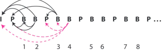
Within each frame interval windowF, we find the worst-case

I P B B P B B P B B P B B P . . .

1 2 3 4 5 6 7 8

Fig. 7. GOP decoding order with possible replacements for B frames if dropped.

every value f, such that 0≤f ≤F. Here f is the number of

frames that were dropped in the frame interval F. Therefore,

we construct the worst-case quality surface Qu_{(f,F). This} procedure is shown in Algorithm 2.

TheMSEmaxstructure containing the maximum MSE values

for B frames is calculated taking all possible concealment frames into consideration. For example, let us take the order of frames in group of pictures (GOP) as shown in Fig. 7. In particular, for the 4th B frame, there are three different possible concealment frames. If the 3rd B frame is not dropped, then it will replace the 4th B frame. If the 3rd B frame is dropped, then the P/I frame will replace 4th B frame in that order. Since P frames are not dropped in our setting, P frame replaces the

4th B-frame if the 3rd B frame is lost. Therefore, MSEmax is

constructed taking all such possible concealment frames. Lines 1 and 2 record the indices of the B frame in the GOP decoding order and then sort the frames in decreasing order

of the MSE values in MSEmax structure, while retaining the

original indices after sorting. For each frame interval window

F, the frame index ranges fromi to i+F−1 wherei is the

variable used for sliding across the video clip. We search for

the F frames within this index range from the sorted MSE

structure shown as MSEmaxsort (Line 3). We slide the window

across the entire video clip and find the F frames for each

i. These quantities are stored in the structureMSEmax(i,n,F)

where 0≤n≤F. The upper bound on MSE is then computed

by searching for the maximum value across all windows of size

F and for every drop count f which ranges from 0≤ f≤F

(Line 4). Once the upper boundMSEu(f,F)is computed, the worst-case quality surfaceQu_{(f,F)can be computed as given}

Algorithm 2Computing worst-case quality surface for a video clip

Input: MSEmax - Maximum MSE values for B frames if

replaced by possible preceding I/P frames. MSE values for I/P frames are set to 0.

Output: Qu_{(f,F)- Worst-case quality surface, f is the}

num-ber of frames dropped in a frame interval ofF

1: Record the frame indices

2: SortMSEmax structure in descending order preserving the

frame indices→MSEmaxsort

3: FindF values within frame index rangeito(i+F−1)in MSEmaxsort:∀i,∀F and 1≤i≤Ntot−F+1 and 0≤F≤ Ntot →MSEmaxF(i,n,F)where 0≤n≤F

4: MSEu(f,F) =max

∀i

Pf

n=0

MSEmaxF(i,n,F) 5: Qu(f,F) =10×log10(₍255_MSE×255u_(f,×_FF₎₎)

in Line 5.

It can be observed from Algorithm 2 that the time complex-ity of computing worst-case qualcomplex-ity surface isO(N_tot3 ).

VI. CASESTUDY(MPEG-2 DECODER)

In this section, we evaluate our proposed analytical frame-work using an MPEG-2 decoder application. In this case study, the MPEG-2 decoder tasks are mapped onto the two PEs in the MPSoC architecture shown in Fig. 2. The tasks mapped are Variable Length Decoding (VLD), Inverse Quantization (IQ), Motion Compensation (MC) and Inverse Discrete Cosine

Transform (IDCT). VLD and IQ are mapped to PE1while MC

and IDCT are mapped to PE2. According to our setup, each buffer in Fig. 2 is composed of two buffers (as shown in Fig. 4) to separate the B frames from I/P frames. We only analyze the drops for B frames and therefore, we analyze only the B frame buffer. The buffer used for I/P frames is not analyzed here because it can be done using conventional Network Calculus

techniques ([2]). PE1 is allocated a frequency of 40 MHz,

whereas PE2is allocated a frequency of 100 MHz. The various

B frame buffer sizes used in the first stage are set to be 30 frames, 60 frames, 90 frames, 120 frames and 150 frames. The B frame buffer sizes used in the second stage are the same as in the first stage. However, the analysis of drops in the second stage is done by fixing the first stage buffer size to 90.

The cycle requirements for each task on the model of a processor was obtained using the SimpleScalar simulator ([1]). Here, we use a MIPS-like processor model using the Portable instruction set architecture (PISA). We use three MPEG-2

video clips in our experiments, namely, susi 080, time080

andorion2. The first two videos are taken from [12], where

both have a total of 450 frames, i.e., Ntot =450 with 1320

macroblocks (MBs) in each frame. The first clip is a motion video and the second one is a still video. The third video, taken from [13], is a combination of both motion and still frames. It has a total of 1171 frames, i.e.,Ntot=1171 with 1350 MBs in each frame. All the three video clips have a bit rate of 8 Mbps.

A. First stage results

The first stage involves computing the drop bounds of

the B frame buffer at PE1 (denoted by Bf in1), which is

of size Bmax1. The arrival curves at the input of Bf in1 are

αf in1 = [αu_{f in1},αl_{f in1}] as computed in Section 3. Similarly,

the service curves offered to the frames in Bf in1 are

βf in1= [β_{f in}u ₁,β_{f in}l ₁].

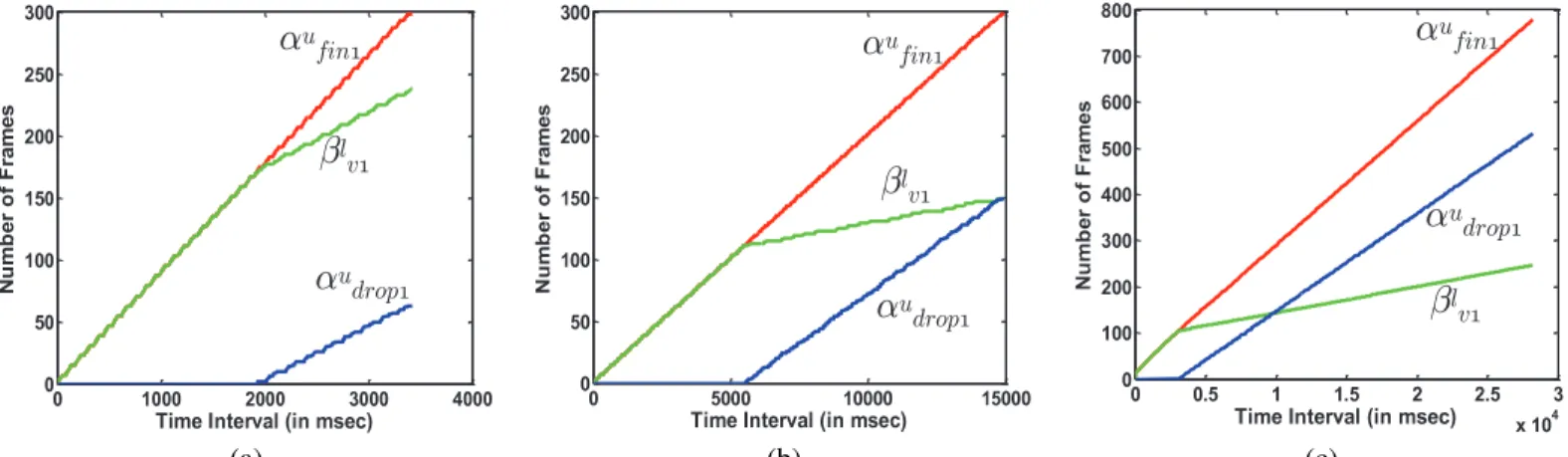
Arrival curve, virtual processor service curve and drop bound (in time intervals): Fig. 8 shows the upper arrival curves of the B frames (αu

f in1) and the lower service curve of the virtual processor (βl

v1) for the three clips (computed using the techniques in Section 4). The worst case drop bound,

αu

drop1, obtained as a result of Lemma 4.3 is also shown

in the three plots. In this experiment, Bmax1=90, which

is in frames. It can be observed from the plots that, until a certain time interval, the drop bound is zero. After that interval, however, the drop bound increases. This is expected

! "# $ % & '(

)

*+

,

-.

/

,

0

)+

1

®

¯

®

2 3444 56666 78999

:

;< =>> ?@A BCC DEF GHH

I JK L MNOL PQR STJN K ULV W XY

Z

[\

]

^

_

`

]

a

Z\

b

®

¯

®

c def g hij k lmn o p q rs

t

u vv w xx y zz { || } ~~  €€  ‚‚

… †‡ ˆ ‰Š‹ˆ Œ Ž  †Š ‡ ‘ ˆ’ “ ”•

–

—˜

™

š

›

œ

™



–˜

ž

®

¯

®

(a) (b) (c)

Fig. 8. Generation of time interval based drop bound curves (αu

drop) from the upper arrival (αu) and lower virtual processor service (βvl) curves. HereBmax=90. The three plots are for clips (a)time080, (b)susi080 and (c)orion2.

Ÿ  ¡ ¡ ¢££ ¤ ¥¥ ¦§§ ¨©©

ª

«¬ ­® ¯° ±² ³´´

µ ¶· ¸ ¹ º »¼½ ¾ ¿ ÀÁÂ

Á

Ã

ÃÄ

Å

Æ

Ç

È

Ä

Á

É

Ê

ËÌÍÎÏÐÑÒÍÎ ÓÔÕ Ö×ØÙÔÚÛ

ÜÝ Þßà á â ã

äÝ Þßà å æç è

é êëë ìíí îïï ðññ òóó

ô

õö ÷øø ùúû üýý

þ ÿ

!"#$

%& '() * + ,

%& '()* -. ,

/ 011 233 455 677 8999 :;<<

=

>?? @AA BCC DEE FGG HII

J KLM N O PQ R S T UVW

V

X

XY

Z

[

\

]

Y

V

^

_

` abcdefgbc h ij k lmniop

q r stu v w x

q r stuv y z x

(a) (b) (c)

Fig. 9. Comparison of Analytical and Simulation results of worst-case drop bound for two buffer capacities. The three plots are for clips (a)time080, (b)susi080 and (c)orion2.

{ | } ~  €

(a) (b) (c)

Fig. 10. Worst case quality surface (Qu in dB) for the clips (a)time080, (b)susi080 and (c)orion2.

because the buffer size of 90 frames is insufficient to avoid buffer overflow. It is also seen that βl

v1followsαuf in1until the

former rises above the buffer size. From there onwards, βl

v1

starts dropping behind αu

f in1 as frames are dropped. Another

interesting observation is that for still video time080, βl

v1 is closer to αu

f in1 and hence, the drop bound is lower when

compared to clips susi080 and orion2. However, it is

interesting to notice that the video clip orion2 has a higher

drop bound value than susi 080. This is because the service

required by the frames in orion2 is higher than the the

service required by the frames in susi 080 as the former has

more macroblocks per frame.

Validation of drop bounds (in frame intervals) with sim-ulation: We validate the drop bounds [αu

dropF1] computed using our analytical framework with the ones obtained by simulation. Here, the drop bound is in frame intervals and not time intervals. Onceαu

drop1is computed,[αdropFu 1] can be computed according to Lemma 4.4. We show the comparison between simulation and analytical results for two buffer sizes, Bmax1=60 and Bmax1=120. It is clear from Fig. 9 that the analytical results emulate the simulation results very closely. Our analytical results are a little pessimistic because they consider the worst case in all the frame windows, whereas

the simulation result depicts only one continuous run. It is also seen that[αu

dropF1]decreases as the buffer size increases, which is expected. It is interesting to note that the difference between simulation and analytical results is greater inorion 2 than in the other two videos. The reason for this behaviour is thatorion2 is a larger clip and the variability in the required

service is larger. In the case of susi 080 and time080, the

variability in required service is limited.

Worst-case quality surface: The worst-case quality surface computed using Algorithm 2 is presented for the three clips in Fig. 10. It is observed that the worst-case quality surface is an exponential surface as it represents the PSNR value for various frame drops within a frame interval. In all theQuplots shown, the PSNR value is highest when the least number of frames are dropped in the largest frame interval. The PSNR surface keeps falling from that point as the number of frames dropped increases and the frame interval decreases. This surface is an architecture independent feature of the video clips. According

to Fig. 10,time080 has the highestQu_{values among all the}

video clips.

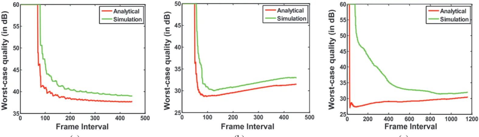
Comparison ofqu with simulation results: The comparison of frame interval based worst-case quality (qu) is presented in Fig. 11(a), (b) and (c) for the three clips. The immediate observation from the plots is that, for orion2, there is a con-siderable deviation of the analytical result from the simulation results in the lower frame intervals. This is because the clip is large and the analytical model considers the worst case across the entire clip. On the other hand, the simulation based result is the outcome of one continuous run. Therefore, if the worst case does not occur in the beginning of the clip, the deviation is large. However, the interesting point is that the curves converge closer towards the higher frame intervals. Hence, it is useful to use the higher frame intervals to explore the quality-buffer design space because they help to reduce the overestimation in buffer size required. However, even if overestimation exists, buffer dimensions can be reduced for a lower tolerable quality if the zero loss constraint need not be strictly adhered to.

Variation of worst-case quality with buffer size: The

variation of qu with buffer size is shown in Fig. 12. As is

expected, in Fig. 12(a), (b) and (c),quvalues increase as the

maximum buffer capacity Bmax1 is increased. We explore the

variation for five buffer sizes as shown in Fig. 12. However, it is interesting to note here that, in all the three curves, the qu _{value rises infinitely at some frame interval value. This is} because below that frame interval, no frame drop is possible with the corresponding buffer size and therefore, the quality is maximum. As the first drop happens, the worst-case quality reduces and assumes a finite value. Another interesting aspect that this work highlights is shown clearly in Fig. 12. In the higher frame intervals, the worst-case quality values are very close to each other for different buffer sizes. This property could be exploited to reduce buffer dimensions for a small

trade-off in qu. For example in Fig. 12(a), if 40−45dB is

an acceptable value for qu, in a frame interval of 450, then

Bmax1=90 can be chosen rather than Bmax1=120 in order

to reduce the maximum buffer required. For an acceptable qu=30−35dB, it is seen in Fig. 12(b) that the least buffer size of 30 can be chosen for a frame interval of 450. Similar

tradeoffs are evident in the third curve as well. B. Second stage

The second stage involves processor PE2 and again two

buffers. The frequency allocated to PE2 is 100 MHz. Again, we do not consider the I/P frame buffer, but analyze drop bounds for the B frame buffer only. Therefore, the resource parameter that we include for the analysis of the second stage is the buffer, labeled by Bf in2, which has size Bmax2. The arrival curves at the input ofBf in2areαf in2= [αuf in2,αlf in2]as computed in Section 3. Similarly, the service curves offered to the frames in Bf in2 are βf in2= [βu_{f in2},βl_{f in2}]. The detailed results are presented in [5].

C. Buffer savings

In this analysis, we highlight the significance of our math-ematical framework. The final goal of the framework was to trade-off buffer size with quality. In the earlier results, we have seen that as the maximum buffer capacity is reduced, the quality reduces due to frame drops. However, if the resultant quality after frame drops is within tolerable limits, we can achieve significant savings in buffer. We present this result in Table I. The savings shown consider drops only in the first stage. We find the buffer saving using Bitl(Bnd)−Bitu(Bd). Here,Bnd is the buffer size (in frames) required for no drops andBdis the buffer size (in frames) which allows drops within the tolerable quality shown in Table I. Further, Bitu(F) and

Bitl(F)are the maximum and minimum number of bits inF

consecutive frames, respectively. It is known from multimedia literature that a PSNR value of 30-50 dB is an acceptable output quality. Hence, we vary the tolerable quality from

30-40 dB in steps of 5 dB. The×symbol against the cliptime080

indicates that the quality never drops to 30 dB even if all the

B frames are dropped. We can see from Table I thattime080

shows more savings in terms of percentage when compared to the other two video clips. This is becausesusi080 andorion2 require a higher buffer size (in terms of Megabits) without any frame drops. Therefore, their savings (in percentage) is less.

TABLE I

BUFFER SAVINGS FOR THE THREE VIDEO CLIPS WITH QUALITY VARIATION

Buffer savings clip susi 080 time 080 orion 2 PSNR (in dB)

In Megabits

30 25.88 × 49

35 3.53 5.09 6.16

40 0.15 1.97 1.3

In percentage

30 28.6% × 29.1%

35 3.9% 39.4% 3.6%

40 0.16% 15.5% 0.77%

VII. CONCLUDINGREMARKS

In this paper, we study the effects of frame drops in a multiprocessor system-on-chip platform running video de-coder applications. Towards this objective, we propose a novel mathematical model to compute the worst-case drop bound in a MPSoC architecture with finite buffers. This analytical

 ‚ƒƒ „…… †‡‡ ˆ‰‰ Š‹ ‹ Œ Ž ‘ ’“ ”” •– — ˜ ™š›œž™š Ÿ  ¡ ¢ £¤¥ ¦ §

¨ ©ª « ¬ ­® ¯¬ ©° ª ± ²³ ´ µ ¶· ¸ ¹ µ º » ¼ ¹ ½ ¾ ¶¿ À ¾Á  à Ä

Å ÆÇ Ç È ÉÉ ÊË Ë ÌÍ Í ÎÏ Ï ÐÑ

ÒÓ ÔÕ Ö× ØÙ

ä åæ ç èé êåë ì

í îï ð ñ òó ô ñ îõ ï ö ÷ø ù ú ûü ý þ ú ÿ þ û ! "# $$ %& ' ( )*+,-.)* / 01 2 34506 7

8 9: ; < => ? < 9@ : A BC D E FG H I E J K L I M N FO P NQ R S T

(a) (b) (c)

Fig. 11. Comparison of analytical and simulation results of worst-case quality (qu_{) forB}

max1=30 for three clips (a)time080, (b)susi080 and (c)orion 2.

U VWW XY Y Z[ [ \ ]] ^ _ ` a b c d e f f g h

i jk l m no pm jq k r st uv wx y zv { |} z ~  w€  ‚ ƒ „ … †‡ ˆ ‰ Š ‹ Œ  Ž  ‘ ’ “ ” • –— ˜ ™ š › œ  ž Ÿ   ¡ ¢ £ ¤ ¥ ¦ §¨ © ª « ¬ ­ ® ¯

° ± ²² ³´´ µ¶¶ ·¸ ¸ ¹º

»¼ ½¾ ¿À ÁÂ

à ÄÅ Æ Ç ÈÉ ÊÇ ÄË Å Ì ÍÎ Ï Ð ÑÒ Ó Ô ÐÕ Ö× Ô Ø Ù ÑÚ Û ÙÜ Ý Þ ß àá â ã ä å æ ç è é ê ë ì í î ï ðñ ò ó ô õ ö ÷ ø ù ú û ü ý þ ÿ

! " # $% &# ' ! ( )* + , -. / 0 , 1 23 0 4 5 -6 7 58 9 : ;

< = >?@ A BC D E FGH I JK L M NOP Q RS T UVWX Y Z[\ ] ^_`a b cde

(a) (b) (c)

Fig. 12. Variation of worst case quality (qu) with different buffer sizes for the clips (a)time080, (b)susi080 and (c)orion2.

model helps in exploring the buffer-quality design space by analyzing the worst-case quality when frames are dropped. One important aspect of this work is that we can explore the buffer-quality design space by trading off a significant buffer area for a tolerable loss in quality. In future, we would like to use our analytical framework to explore trade-offs with other important system parameters like peak temperature.

REFERENCES

[1] T. M. Austin, E. Larson, and D. Ernst. Simplescalar: An infrastructure for computer system modeling.IEEE Computer, 35(2):59–67, 2002. [2] J. Y. Le Boudec and P. Thiran. Network Calculus: A Theory of

Deterministic Queuing Systems for the Internet, volume LNCS 2050. Springer, 2001.

[3] M Coenen, S. Murali, A. Radulescu, K. Goossens, and G. D. Micheli. A buffer-sizing algorithm for networks on chip using tdma and credit-based end-to-end flow control. In 4th International Conference on Hardware/Software Codesign and System Synthesis (CODES+ISSS), pages 130–135, 2006.

[4] A. Dua and N. Bambos. Buffer management for wireless media streaming. InGLOBECOM, pages 5226–5230, 2007.

[5] D. Gangadharan, L. T. X. Phan, S. Chakraborty, R. Zimmermann, and I. Lee. Technical report. http://eiger.ddns.comp.nus.edu.

sg/pubs/TRC6-11.pdf.

[6] J. Hu, U. Y. Ogras, and R. Marculescu. System-level buffer allocation for application-specific networks-on-chip router design. IEEE Transaction on Computer-Aided Design of Integrated Circuits and Systems (TCAD), 25(12):2919–2933, 2006.

[7] D. Isovic and G. Fohler. Quality aware mpeg-2 stream adaptation in resource constrained systems. In16th Euromicro Conference on Real-Time Systems (ECRTS), pages 23–32, 2004.

[8] M. Kalman, E. G. Steinbach, and B. Girod. System-level buffer allocation for application-specific networks-on-chip router design.IEEE Transactions on Circuits and Systems for Video Technology, 14(6):841– 851, 2004.

[9] A. Maxiaguine, S. Chakraborty, and L. Thiele. Dvs for buffer-constrained architectures with predictable qos-energy tradeoffs. In3rd International Conference on Hardware/Software Codesign and System Synthesis (CODES+ISSS), pages 111–116, 2005.

[10] A. Maxiaguine, S. Kunzli, S. Chakraborty, and L. Thiele. Rate analysis for streaming applications with on-chip buffer constraints. In9th Asia and South Pacific Design Automation Conference (ASP-DAC), pages 131–136, 2004.

[11] A. Maxiaguine, S. Kunzli, L. Thiele, and S. Chakraborty. Evaluating schedulers for multimedia processing on buffer-constrained soc plat-forms. IEEE Design & Test of Computers, 21(5):368–377, 2004.

[12] Mpeg-2 benchmark videos. ftp://ftp.tek.com/tv/test/

streams/Element/MPEG-Video/625/.

[13] Hubblesource mpeg benchmark videos. http://hubblesource.

stsci.edu/sources/video/clips/index_2.php.

[14] A. Nandi and R. Marculescu. System-level power-performance analysis for embedded systems design. In38th Design Automation Conference (DAC), pages 599–604, 2001.

[15] B. Raman, S. Chakraborty, O. W. Tsang, and S. Dutta. Reducing data-memory footprint of multimedia applications by delay redistribution. In 44th Design Automation Conference (DAC), pages 738–743, 2007. [16] J. Ray and P. Koopman. Data management mechanisms for embedded

system gateways. InDSN, pages 175–184, 2009.

[17] W. Tu, W. Kellerer, and E. Steinbach. Rate-distortion optimized video frame dropping on active network nodes. In Packet Video Workshop, 2004.

[18] G. Varatkar and R. Marculescu. Traffic analysis for on-chip networks design of multimedia applications. In39th Design Automation Confer-ence (DAC), pages 795–800, 2002.

[19] A. Vishwanath, P. Dutta, M. Chetlu, P. Gupta, S. Kalyanaraman, and A. Ghosh. Perspectives on quality of experience for video streaming over wimax. ACM SIGMOBILE Mobile Computing and Communications Review, 13(4):15–25, 2010.

[20] L. Zhang and H. Fu. Dynamic bandwidth allocation and buffer dimensioning for supporting video-on-demand services in virtual private networks. Computer Communications, 23(14-14):1410–1424, 2000.