Smith_unc_0153D_15224.pdf

(1)

MODEL SELECTION FOR NONNESTED LINEAR MIXED MODELS

Ch´

e L. Smith

A dissertation submitted to the faculty of the University of North Carolina at Chapel Hill

in partial fulfillment of the requirements for the degree of Doctor of Philosophy in the

Department of Biostatistics in the Gillings School of Global Public Health.

Chapel Hill

2015

Approved by:

Lloyd

J. Edwards

Peggye

Dilworth-Anderson

Bahjat

Qaqish

Pranab

K. Sen

(2)

c

2015

Ch´

e L. Smith

(3)

ABSTRACT

Ch´

e L. Smith: Model Selection for Nonnested Linear Mixed Models

(Under the direction of Lloyd J. Edwards)

(4)

To my loving parents:

Patricia Kornegay Smith and Calvin Miles Smith, Jr.;

and to my late grandparents:

Dr. Hobert Kornegay, Jr. & Mrs. Ernestine Price Kornegay,

(5)

ACKNOWLEDGMENTS

(6)

(7)

LIST

OF

TABLES

.

x

1

1.1 Introduction

.

1

0.2 The Linear Mixed Effects Model . . . .

2

1.3 Model

Selection

in

the

Linear

Mixed

Model

(LMM)

.

4

1 .3.1

Selecting

among

Nested

Models

.

7

1 .3.2

Selecting

among

Nonnested

Models

.

8

1 .4

Testing

Separate

Hypotheses

in

the

Linear

Mixed

Model

.

11

1 .4.1

The

Cox

Test

of

Separate

Hypotheses

.

11

1 .4.2

Multivariate

Linear

Regression

.

24

1 .5

Using

Information

Criteria

to

Distinguish

Nonnested

LMMs

.

28

1 .5.1

Commonly

used

information

criteria

.

29

1 .5.2

The

Extended

Information

Criterion

(EIC)

.

33

1 .6

Summary

.

35

0.7 Introduction

.

37

0.8 Review

of

Cox

methodology

.

40

2.3 Formulating

the

Cox

Test

of

Nonnested

Hypotheses

for

LMMs with nonnested fixed effects . . . .

43

(8)

2.3 .2

Deriving

T

2

,

computing

V

ar(T

2

),

and

deriving

the distribution of

T2

. . . .

50

2.4 Application

to

Data

.

53

2.4 .1

Comparing

nonnested

fixed

effects

models

in the NC EPESE data . . . .

54 0.10.2 Specification of LMMs with nonnested fixed effects . . . .

55

2.4.3 Results

.

56

2.5 Discussion

and

Conclusions

.

58

3.1 Introduction

.

60

3.1.1 Common

covariance

structures

in

the

LMM

.

62

3.1.2 Selecting

among

nonnested

covariance

structures

.

65

3.2 Cox

Test

of

Separate

Hypotheses

for

LMMs

with

Nonnested Random Effects . . . .

66

3.2.1 Application

to

Data

.

71

3.3 Discussion

.

74

4.1 Introduction

.

75

4.2 Applying

the

EIC

to

nonnested

models

arising

from

repeated

measures

data

.

76

4.3 EIC

for

Nonnested

Models

from

Sections

2.4.2 and

3.2.1 .

.

79

(9)

(10)

LIST OF TABLES

1 Cox test Decision Rules

. . . .

42

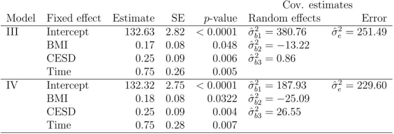
2 Summary of NC EPESE data . . . .

56

3 Fit statistics for Models 1 and 2 . . . .

57

4 Model Estimates, SEs, and

p-values . . . .

57

5 Estimates of

T

1

and

T

2

. . . .

58

6 Common LMM covariance structures . . . .

62

7 Model fit statistics . . . .

72

8 Model Estimates, SEs, and

p-values . . . .

73

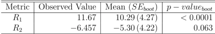
9 Estimates of

R

1

and

R

2

. . . .

74

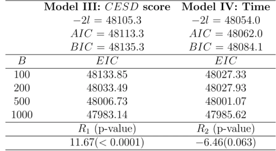
10 EIC

values for models with nonnested fixed effects . . . .

81

(11)

CHAPTER 1: INTRODUCTION AND LITERATURE

REVIEW

1.1 Introduction

Selecting an adequate and parsimonious model is an important, yet often neglected,

aspect of data analysis and research. Over the past few decades, the majority of research

in model selection has centered around linear regression and other univariate linear models.

Any work beyond that class of models has involved the extension of existing model selection

methods applied to regression and univariate linear models (e.g., likelihood ratio tests,

R

2

coefficient, information criteria) to more complex types of models, with little investigation

of the robustness of these methods after extension. Even more rarely have model selection

techniques for the linear mixed model been thoroughly examined. Here, an attempt to

extend the capability to select among nonnested linear mixed models is made.

(12)

of these two components. Well-developed techniques exist for comparing models with nested

mean and/or covariance structures, mostly following from Neyman-Pearson (Neyman and

Pearson, 1933) theory. On the other hand, formal approaches to compare models lacking

this nested structure (or

nonnested

models) have not been developed.

This review highlights important findings from the literature on model selection for the

linear mixed model - with special attention given to the case of nonnested models - and

illuminates some opportunities for methodological improvement.

In the next section, a

detailed specification of the linear mixed model is introduced with specific notation to be

used throughout this document. Subsequent sections review the history of model selection

techniques for univariate linear models, and their extension to multivariate and correlated

data. Special attention is paid to the case of comparing nonnested linear mixed models,

which has received little attention. Specifically, two general approaches to model building

and selection among nonnested linear mixed models are highlighted - hypothesis testing

and the use of information criteria. Particularly for the hypothesis testing approach, ties

are made from the econometrics literature which contains applications of selecting among

nonnested models of a similar structure to linear mixed models. Finally, the most important

findings from the literature review are summarized.

1.2 The

Linear

Mixed

Effects

Model

The Linear Mixed Effects Model (referred to hereafter as the

linear mixed model

) is used

to analyze multivariate continuous data, particularly longitudinal data. Consider the linear

mixed model for repeated measures data specified below (Edwards et al., 2008):

(13)

matrix

X

i

is the known and fixed design matrix for person

i, with full column rank

p.

(p

×

1) vector

β

is a vector of unknown, constant population parameters, common to all

subjects. Matrix

Z

Zi, of dimension (ni

×

q), is a known, constant design matrix with rank

q

for person

i

corresponding to the (q

×

1) vector of unknown random effects,

b

i

, while

e

i

is an

(n

i

×

1) vector of unknown random errors. Random effects are assumed to be independent

of random errors, and together they are assumed to follow a normal distribution with mean

0 and variance

V













b

i

e

i













=







Σ

bi

(τ

b

)

0

0 Σ

ei

(τ

e

)







.

In the equation above,

V

(·) is the covariance operator, while both

Σ

bi

(τ

b

) and

Σ

ei

(τ

e

)

are positive-definite, symmetric covariance matrices. Therefore,

V

(y

y

yi) may be expressed as

Σ

i

=

Z

i

Σ

bi

(τb)

Z

0

i

+

Σ

ei

(τe). We assume that

Σ

i

can be characterized by a finite set of

parameters represented by an (r

×

1) vector

τ

, which consists of the unique parameters in

τ

b

and

τ

e

.

For simplicity, we will assume here that all subjects have the same number of repeated

measurements, so that

n

i

=

n

for all subjects, such that

e

i

∼

N

n

(

0 ,

Σ

e

(τ

e

)), where the

(n

×

1) vector

τ

e

collects the

n

unique parameters of

Σ

e

(τ

e

).

Alternatively, we may specify the linear mixed model for all subjects in a stacked

formu-lation as follows:

y

=

X

Xβ

+Z

Z

b

+

e

where

y

= (y

y

0₁

. . . y

y

0_N

)

0

; design mnatrix

X

= (X

X

0₁

. . . X

X

0_N

)

0

;

vector

β

is as specified before;

Z

=

diag

(Z

Z

1

, . . . , Z

Z

N

); vector

b

is as specified before; and

e

= (

e

0₁

. . .

e

0_N

)

0

.

Note the dimensions of

y

y, X

X

X, Z

Z

Z, and

e

are (N n

×

1), (N n

×

p), (N n

×

q), and (N n

×

1),

respectively. Further,

b

∼ N

q

(

0 ,

Σ

bi

(τ

b

)

⊗

I

b

) and

e

∼ N

Nn

(

0 ,

Σ

e

). We have

Σ

e

=

diag

[

Σ

e1

(τ

e

)

, . . . ,

Σ

eN

(τ

e

)]; thus

y

∼ N

(X

X

Xβ,

Σ

) with

Σ

=

V

(y

y) =

y

diag

(

Σ

1

, . . . ,

Σ

N

).

(14)

collection of its complete parameter space

θ, where

θ

= (β

0

,

τ

0

)

0

is a (s

×

1) vector, with

s

=

p

+

r.

1 .

3 Model

Selection

in

the

Linear

Mixed

Model

(LMM)

The selection of an adequate model among suitable candidate models is an essential part

of the model-building process and has been widely studied for the univariate linear model and

other types of models arising from cross-sectional data. Most commonly for linear regression

models, researchers employ forward, backward, and stepwise variable selection procedures.

Ngo and Brand (2002) discussed how the extension of these procedures to the linear mixed

model introduces problems of multiple testing, further complicated by the use of an arbitrary

level of significance. Some methods are ad hoc, and have not been well developed or studied.

This is especially true for the linear mixed model, which requires selection of both a mean

model and a covariance model.

(15)

1. Specify the maximum model to be considered (both in fixed and random effects).

2. Specify a criterion of goodness of fit of a given model.

3. Specify a predictor selection strategy.

4. Conduct the analysis.

5. Evaluate the reliability of the model chosen.

Cheng et al. emphasize that these steps are also appropriate for building univariate,

mul-tivariate, linear, and nonlinear models, along with models for any type of response variable

distribution. Their discussion also follows the assumption that the ’best’ model is contained,

or

nested

, within a maximum model. Of particular interest here is the third item in the above

list. It is important to predetermine a strategy that will lead to fitting a select few models

with as few predictors as necessary to characterize the outcome variable(s). In most cases,

the maximal model rarely ends up being the final model. Ideally, one would implement a

well-planned strategy to select a small number of predictors based on the size of the data

and knowledge of the subject area. For linear regression, it is straightforward to employ

techniques such as forward, backward, or stepwise variable selection. Model selection for the

linear mixed model, however, is more complex and requires attention to its two models - the

mean structure, and selection of random effects and variance components (Liu and Yang,

2008). In the linear mixed model, it is common to keep one aspect of the model fixed in

both models, while using techniques to refine the other model. For example, one may assign

a common covariance matrix to both models and compare models with different sets of fixed

effects.

(16)

and different covariance structures. These categories may be expanded to more specifically

outline the types of linear mixed models that may be compared. One may compare:

1) Nested mean models with:

a. the same covariance structure;

b. different (but nested) covariance structures; or

c. nonnested covariance structures, or

2) Nonnested mean models with:

a. the same covariance structure;

b. different (but nested) covariance structures; or

c. nonnested covariance structures.

The first case listed above - comparing nested mean models - is most commonly considered

(Diggle et al., 1994; Wolfinger et al., 1993). Selection of a favored model is largely based

on extensions of techniques used for univariate linear models, such as likelihood ratio tests,

goodness of fit measures, predictive criteria (R

2

,

P RESS, etc.), and information criteria

(AIC,

BIC, etc.). Existing techniques rely on theories developed by Neyman and Pearson

(1933) or Kullback and Leibler (1951). theory. Virtually all recent reviews of variable/model

selection in the linear mixed model only consider cases of mean models that are nested (Wang

and Schaalje, 2009; Dziak and Li, 2007; Dimova et al., 2011). Here, models are considered

(17)

1.3.1 Selecting

among

Nested

Models

The vast majority of model selection techniques were developed to make comparisons

between pairs of models that follow a nested structure. Models are considered nested when

one model can be obtained by imposing a set of linear constraints on another more general

model. In terms of the linear mixed model, one may consider models with nested fixed

and/or random effects. Models with nested fixed effects are typically compared under

maxi-mum likelihood estimation using likelihood ratio tests,

t

tests, or

F

tests. Models with nested

covariance structures are compared under restricted maximum likelihood (REML)

estima-tion using

χ

2

_{tests. Wang and Schaalje (2009) reviewed several model selection techniques}

involving predictive criteria that were originally designed for selecting among ordinary linear

models. The authors summarize the history of the adjusted

R-squared

R

adj2

(18)

1.3.2 Selecting

among

Nonnested

Models

The second case, where models are nonnested, is seldom addressed. There are varied

scenarios in which candidate models could be considered nonnested. One may consider

comparing models with

nonnested sets of explanatory variables

, where non-linear restrictions

to parameter vectors from both models are required to establish a nested structure between

competing models. Most commonly seen is the case of alternative, positively correlated,

measures of the same concept in nonnested parametric form, where both of which are assumed

to influence some outcome (Cole et al., 2005). For example, Dameus et al. (2002) compared

models with rival econometric theories to expain the same phenomenon. Additionally, one

could compare models with the partially overlapping sets of main effects and with nonested

interactions among explanatory variables. Another manifestation of nonnested models of this

type occurs in models having additive vs. multiplicative interactions; that is, testing absolute

(additive) risk difference vs relative (multipicative) risk (Kalilani and Atashili, 2006). One

may also compare models with

nonnested functional forms

; an example of this case is the

comparison of linear vs. log-linear functions of a continuous outcome variable. One would use

a linear mixed model under the assumption of a Normal distribution for the first function, and

a gamma link for the nonlinear model under the assumption of a non-Normal distribution.

One could also use a generalized estimating equations (GEE) approach in both, but this case

is not explored here.

(19)

the

R

2

_{statistic is most commonly used to compare nonnested models, though traditionally it}

is a goodness-of-fit statistic. Edwards et al. (2008) developed an extension of this technique

to the linear mixed model to determine an association between repeated measurements and

fixed effects. Watnik and Johnson (2002) discuss using a relative efficiency approach to

com-pare nonnested linear regression models and considers globally non-nested models, in which

neither design matrix is a subset of the other. Timm et al. (2002) compared nonnested

models arising from a meta-analysis of six studies investigating the effect of academic

coach-ing on students’ SAT scores. They use a modified Wald test statistic developed in a prior

investigation (Timm et al., 2001) which was shown to be more powerful than the hypothesis

test developed by Cox (1961). The authors do not consider repeated measures data, but they

acknowledge that the use of an information-theoretic approach (using information criteria)

as a suitable alternative to their methodology. That approach is considered here as well, and

discussed in more detail in a later section.

(20)

magnitude of difference between models.

Other notable investigations of comparing nonnested models include Ette (1996), who

compared nonnested (or non-hierarchical) nonlinear mixed models arising from longtiduinal

observations of pharmacokinetic data; particularly, he compared models with the same

co-variates, but one having a different parametric form in each model; the two candidate models

were thus highly correlated, but not nested by earlier definitions. Ette bootstrapped the

log-likelihood difference betweeen candidate models. His investigation illuminates the need

for more research related to bootstrapping correlated data and comparing nonnested models

arising from longitudinal data. Haskard et al. (2010) discussed ways to compare linear mixed

models with nonnested - or

non-stationary

random effects, and used the

AIC

to compare

models. These data were not repeated observations, but rather each vector of observations

contained soil samples from nearby locations so that clusters of observations were correlated

spatially. In another example using linear mixed models, Morrell et al. (2009) describe

how changes in parameterization of time-dependent covariates (mainly, subject’s age) can

influence results of longitudinal models. The authors compared models with nonnested fixed

and random effects, using the

AIC

and

BIC

as selection criteria, noting that models with

nonnested fixed effects cannot be compared using these criteria under REML estimation.

(21)

1.4 Testing

Separate

Hypotheses

in

the

Linear

Mixed

Model

While recent literature has given much attention to model selection for nonnested

regres-sion models and econometrics models, the case of selecting among nonnested linear mixed

models remains severely underexplored. Seminal works of Cox beginning in 1961 and 1962

highlight tests of

separate

families of hypotheses, meaning that one hypothesis (or model)

cannot be obtained as a simple limit of the other; before his works, ad hoc methods were

em-ployed to test separate hypotheses. Since then, Pesaran (1974), Pesaran and Deaton (1978)

and several others have also studied this methodology extensively. Parallel approaches have

also been developed, employing theories such as the encompassing approach Mizon and

Richard (1986), including the J-test (Davidson and MacKinnon, 1993) and Vuong’s Test

(Vuong, 1989). One major disadvantage of these approaches is that the assumption of an

all-encompassing model can become tedious for the linear mixed model, since one must

consider both the mean model and covariance structure. Here, we describe Cox’s Test of

Separate Hypotheses in more detail, providing examples of its implementation, and

outlin-ing some considerations for applyoutlin-ing this approach to compare separate, or nonnested, linear

mixed models.

1.4.1 The

Cox

Test

of

Separate

Hypotheses

(22)

are considered separate due to the definitions of the hypotheses. Conventional techniques

for comparing nested models, such as Wald’s

F

test, do not apply for the comparisons of

nonnested models, as they require restrictions on the models’ parameter spaces that do not

exist, thus making it more difficult to estimate the distribution of the ratio of likelihood

functions. Cox recognized the need to make modifications to recenter the likelihood ratio

and standardize a test statistic with an asymptotically normal distribution. Pesaran and

Weeks (2000) provide a good summary of the motivation behind Cox’s formulation. The

literature following Cox’s two papers has been extensive, but few well-developed techniques

and extensions have been studied or recommended, especially for the linear mixed model.

In the following section, Cox’s methodology is defined and described in more detail.

Notation and Setup

Let

y

= (y

1

, y

2

, . . . y

m

) be an (m

×

1) observed random vector and suppose we are

in-terested in testing the composite null hypothesis,

H

1

, that the probability density function

(pdf) is

f

(y

y

y,

θ

1

) against the composite alternative,

H

2

, that the pdf is

g

(y

y

y,

θ

2

), where

θ

1

and

θ

2

are vectors of dimension (k

1

×

1) and (k

2

×

1), respectively. That is

H

1

:

f

(y

y

y,

θ

1

)

H2

:

g(y

y

y,

θ2)

where

θ

1

∈

Ω

1

⊂

R

k1×1

and

θ

2

∈

Ω

2

⊂

R

k2×1

, where

k

1

, k

2

>

1. Note the following

assumptions:

(i) the parameters

θ

1

and

θ

2

may be treated as varying continuously even when a

compo-nent of say

θ2

is the serial number of the observation at which a discontinuity occurs;

(ii) the values of

θ

1

, or

θ

2

, are interior to Ω

1

, or Ω

2

, so that the type of distribution problem

(23)

Let

l

1

( ˆ

θ

1

) be the maximized log-likelihood function of the model proposed under

H

1

and

l

2

( ˆ

θ

2

) be the maximized log-likelihood function under

H

2

, where ˆ

θ

1

and ˆ

θ

2

are the

maximum likelihood estimates of

θ1

and

θ2, respectively. Cox proposed using the following

test statistic:

T

1

=

l

1

( ˆ

θ

1

)

−

l

2

( ˆ

θ

2

)

−

E

h

l

1

( ˆ

θ

1

)

−

l

2

( ˆ

θ

2

)

i

θ1= ˆθ1

,

(1)

which compares the observed difference of log-likelihoods with an estimate of the

ex-pected difference between log-likelihoods, with expectation taken under

H

1

. In the expected

difference

θ

1

is replaced with its maximum likelihood estimate, ˆ

θ

1

, under

H

1

; other unknown

paramters are also replaced with estimates under the null. Under the null hypothesis, Cox

(1961; 1962) showed the value of

T

1

should be nearly zero, while under

H

2

,

T

1

is presumed to

be negative. Thus, a large negative value of

T1

leads to the rejection of the null hypothesis,

H

1

.

Alternatively, a simplified specification of

T

1

is given by

T

1

= ˆ

l

12

−

E

h

ˆ

l

12

i

θ1= ˆθ1

where ˆ

l

12

=

l

1

ˆ

θ

1

−

l

2

ˆ

θ

2

Furthermore, a different specification of

T

1

is given by

T

1

= ˆ

l

12

−

N

plim

N→∞

ˆ

l

12

N

!

θ1= ˆθ1

.

Replacing the expectation in the second term with a probability limit (plim) allows for

more flexibility when working with complex expressions, especially those involving products

and quotients of random variables. (Dougherty, 2011;

Appendix A

)

A few general remarks are in order (White, 1982):

(24)

assump-tion of separate families, this inequality - representative of the models having nested

structures - may not hold.

(ii) When the components of

y

are independent,

l12

is the sum of

n

independent terms and

an application of the central limit theorem will usually prove the asymptotic normality

of

l

12

. Approximations to the percentage points of

l

12

can then be obtained under both

H

1

and

H

2

.

(iii) The hypotheses

H

1

and

H

2

are considered asymmetrically, and are not assumed to be

the only possible hypotheses.

(iv) The roles of

H1

and

H2

can be interchanged, yielding corresponding test statistic

T2,

where

T

2

=

l

2

( ˆ

θ

2

)

−

l

1

( ˆ

θ

1

)

−

E

h

l

2

( ˆ

θ

2

)

−

l

1

( ˆ

θ

1

)

i

θ2= ˆθ2

.

(2)

Here, expectation is taken under the new null,

H

2

, and

θ

2

is replaced by its maximum

likelihood estimate under

H

2

, ˆ

θ

2

, while all other unknown parameters are replaced by

their estimates under

H

2

.

In order to make inferences using

T

1

and/or

T

2

, one must derive the distribution of these

statistics. Cox established that both test statistics have a limiting distribution that is Normal

with mean 0 and Cox denoted the variances of

T1

and

T2,

V ar(T1) and

V ar(T2), respectively,

by:

V ar(T

1

) =

V

1

(l

12

)

−

G

01

I

−1

1

G

1

and

V ar(T

2

) =

V

2

(l

21

)

−

G

02

I

−1

2

G

2

, where

V

1

(l

12

) is the

variance of the log-likelihood ratio taken under the null hypothesis, and

V

2

(l

21

) is defined

correspondingly for the case where the null and alternative hypotheses are interchanged,

G

1

=

N

∂

∂θ

1

plim

_N→∞

ˆ

l

12

N

G

2

=

N

∂

∂θ

2

(25)

and

I

1

and

I

2

are the information matrices corresponding to

θ

1

and

θ

2

, respectively.

Thus, for any pair of hypotheses, two tests may be constructed.

In the following sections, we derive

T1

and

T2

and their corresponding distributions for a

pair of linear mixed models with nonnested fixed effects.

Coulibaly and Brorsen (1999) first proposed using a parametric bootstrap to estimate

the distribution of test statistics under the corresponding null hypothesis, showing that this

technique helped achieve correct test size and higher power, especially in small samples.

Dameus et al. (2002), Monfardini (2003), and Godfrey (2007) also establish a need for

bootstrapping the distributions of statistics for comparing various types of models applied

to econometrics analyses. Huber (1967) discusses the behavior of maximum likelihood

es-timates under nonstandard conditions, but not much of the literature following Cox’s work

adequately addresses the distribution of test statistics and their limitations under different

variance estimates.

Definition of Separate Families

The hypotheses,

H

1

and

H

2

, are separate in the sense that an arbitrary simple hypothesis

H1

cannot be obtained as a simple limit hypothesis in

H2. That is,

f

(y, θ1) and

g(y, θ2)

represent separate families in that an arbitrary value of

θ

1

cannot be approximated arbitrarily

closely by

g(y, θ

2

).

Existing examples

In his seminal works, Cox presented several scenarios in which one could apply his

method; selected examples are described below.

Lognormal vs. Exponential

In this example, the null hypothesis assumes a model

fol-lowing a lognormal distribution; that is,

f

(y) =

1

y √

2πσ2

e

(lny−µ)2

2σ2

. The alternative

(26)

T

1

=

n

log

ˆ β

βˆα

, where

β

αˆ

=

e

ˆ α1+α2

2

, and

V ar(T

₁

) =

n e

α2ˆ

−

1 −

α

ˆ

₂

−

1 2

α

ˆ

2 2

. Not shown here

or in other examples, it is trivial to derive the statistic

T

2

which assumes

g(y) is the null

hypothesis,

f(y) as the alternative, along with an expression for its variance.

Alternative

forms of independent variables

Consider comparing the following sets of models

y

=

aα

y

=

bβ

or

y

=

α

1

+

α

2

x

y

=

β

1

+

β

2

log

x

Cox (1961) explained that the two pairs of models above are from a problem considered

by Hotelling (1940), and expounded upon in Williams (1959); Cox demonstrated the need

for more theoretical exploration for nonnested models of this type.

Alternative forms of the dependent variable

E

(log

y) =

aα

E

(y) =

aβ

(27)

Poisson vs. Geometric distributions

f

Y

(y) =

e

−α

α

y

y!

(y

= 0,

1,

2, . . .) ;

g

Y

(y) =

β

y

(1 +

β)

y+1

(y

= 0,

1,

2, . . .)

Cox (1962) explained that this example, demonstrating the comparison of exact versus

asymptotic statistical theory, results in a test statistic

T

1

=

−Σ log

Y

i

! +

nl

f

Y

¯

, where

l

f

(·)

is the log-likelihood function of

fY

(y), which assumes the model

fY

(y) is the null hypothesis

and

g

Y

(y) is the alternative.

Demand analysis models with nonnested functional forms

Dameus et al. (2002) explored comparisons of nonnested demand analysis models (US meat

demand), and showed that using a Cox test with a parametric bootstrap was more powerful

than using encompassing tests. The authors compared the following two demand analysis

models.

First-difference AIDS model:

∆s

i

=

τ

i

+

4

X

k=1

θ

ik

D

k

+

4

X

j=1

γ

ij

∆ ln (p

j

) +

β

i

[∆ ln (x)

−

∆ ln (P

)]

,

i

= 1, . . . ,

4 Rotterdam model:

¯

s

i

∆ ln (y

i

) =

τ

i

+

4

X

k=1

θ

ik

D

k

+

4

X

j=1

γ

ij

∆ ln (p

j

) +

β

i

"

∆ ln (x)

−

4

X

j=1

¯

s

j

∆ ln (p

j

)

#

Multinomial Probit vs. Multinomial Logit Model

(28)

Multinomial probit model:

u

p_ij

= x

0_i

α

j

+

ν

ij

(ν

i

) = (ν

i1

, . . . , ν

iJ−1

)

0

≈

i.i.d.N

(0,

Σ)

, j

= 1, . . . , J

−

1,

Multinomial logit model:

u

l_ij

= x

0_i

δj

+

ηij

(ηi) = (ηi1, . . . , ηiJ−1)

0

≈

i.i.d.Logistic

(0,

Λ)

, j

= 1, . . . , J

−

1,

To date, this methodology has not been extended to the case of comparing linear mixed

models with nonnested fixed and/or random effects. The last two of the extensions outlined

below (Pesaran (1974) and Araujo et al. (2005)) provide the most adequate framework for

developing test statistics for nonnested linear mixed models. We consider these extensions

in more detail in the sections below.

Univariate Linear Regression

Pesaran (1974) derived test statistics to compare two univariate linear regression models

with nonnested fixed effects. This section summarizes the formulation. Suppose there are

data for

N

independent subjects; consider the following hypotheses:

H

1

:

y

=

X

Xβ

1

+

eee

1

;

eee

1

∼ N

(

0 , σ

12

I

N

)

H2

:

y

=

W

β2

+

eee2;

eee2

∼ N

(

0 , σ

₂2

I

N

).

(29)

design matrix

W

and random errors also distributed normally with mean

0 and variance

σ

₂2

I

N

, with

I

N

defined as before. Furthermore, assume that

X

and

W

are not nested; that

is, all of columns of

X

cannot be obtained from those of

W

and vice versa. For simplicity,

we assume that

X

and

W

have the same dimensions. Recall from the discussion of Levy

and Hancock (2007) that most often considered is the case of partially overlapping models,

where there may be some variables in common between the models but neither design matrix

is a subset of the other. We denote the collections of unknown parameters of each model

as

θ

1

= (β

10

, σ

12

)

0

and

θ

2

= (β

20

, σ

22

)

0

, both vectors having dimension (p

+ 1

×

1). Pesaran

required that the following three limits exist and are finite.

lim

N→∞

1 N

X

0

X

=

Σ

X0_X

lim

N→∞

1 N

W

0

W

=

Σ

W0_W

lim

N→∞

1 N

X

0

W

=

Σ

X0_W

where the matrices

Σ

X0_X

and

Σ

_W0_W

are nonsingular and

Σ

_X0_W

6=

0 . All matrices are of

dimension (N

×

N

).

Formulation of expressions for

T1

and

V ar(T1)

First, the log-likelihood functions corresponding respectively to the linear models given

in hypotheses

H

1

and

H

2

are defined below:

l

1

(θ

1

) =

−

N

2 log (2πσ

1

2

₎

₋

1 2σ

12

(y

y

−

X

Xβ

1

)

0

(y

y

−

X

Xβ

1

)

l2

(θ2) =

−

N

2 log (2πσ2

2

)

−

1 2σ

22

(y

y

−

W

β2)

0

(y

y

−

W

β2)

,

(30)

and the maximum log-likelihood ratio (or difference in log-likelihood functions) by ˆ

l

12

=

l

1

ˆ

θ

1

−

l

2

ˆ

θ

2

, recall the formula for

T

1

given by:

T

1

= ˆ

l

12

−

N

h

plim

_N→∞

ˆ

l

12

/N

i

θ= ˆθ1

,

with

plim

taken under the assumption of

H

1

. The maximum likelihood estimates of

θ

1

and

θ

2

, given by ˆ

θ

1

and ˆ

θ

2

, respectively, are defined as follows.

First, ˆ

θ

₁0

=

ˆ

β

₁0

,

σ

ˆ

₁2

, where

ˆ

β

1

= (X

X

0

X

X)

−1

X

0

y

y,

ˆ

σ

₁2

=

y

0

_(I

N

−

M

X

)

y

N

.

(N

×

N

) matrix

I

N

is defined as before, and (N

×

N) matrix

M

X

is given by

M

X

=

X

(X

X

0

X

X)

−1

X

0

.

Next, ˆ

θ2

=

ˆ

β2

,

σ

ˆ

₂2

, where

ˆ

β

2

= (W

W

0

W

)

−1

W

0

y

y,

ˆ

σ

₂2

=

y

0

₍

_I

N

−

M

WWW

)

y

N

.

Here, (N

×

N

) matrix is defined by

M

W

=

W

(W

W

0

W

)

−1

W

0

.

Now,

l

12

=

N

2 log (σ

2 2

_/σ

12

) +

1

2 σ

2−2

(y

y

−

W

β

2

)

0

(y

y

−

W

β

2

)

−

σ

1−2

(y

y

−

X

Xβ

1

)

0

(y

y

−

X

Xβ

1

)

.

(31)

likelihood estimates as defined above.

ˆ

l

12

=

N

2 log (ˆ

σ

2 2

/ˆ

σ

2 1

) +

1

2 ˆ

σ

₂−2

y

−

W

β

ˆ

2

0

y

−

W

β

ˆ

2

−

σ

ˆ

−2₁

y

−

X

β

ˆ

1

0

y

−

X

β

ˆ

1

=

N

2 log (ˆ

σ

2 2

/ˆ

σ

2 1

) +

1

2 (y

y

0

(

I

−

M

W

)

y

y)

−1

y

−

W

β

ˆ

2

0

y

−

W

β

ˆ

2

−

(y

y

0

(

I

−

M

X

)

y

y)

−1

y

−

X

β

ˆ

1

0

y

−

X

β

ˆ

1

=

N

2 log (ˆ

σ

2 2

/ˆ

σ

2 1

) +

1

2 (y

y

0

(

I

−

M

W

)

y

y)

−1

(y

y

0

(

I

−

M

W

)

y

y)

−

(y

y

0

(

I

−

M

X

)

y

y)

−1

(y

y

0

(

I

−

M

X

)

y

y)

=

N

2 log

ˆ

σ

2₂

ˆ

σ

2

1

Determining the second term of

T

1

requires finding the probability limit (plim) of ˆ

l

12

under the assumption that the null hypothesis is the true model. First, by definition, we

know that plim

_N_→∞

(ˆ

σ

2

1

) =

σ

12

. Assuming

H

1

is the true model, Pesaran (1974) determined

the expected value of ˆ

σ

2

, denoted by ˆ

σ

212

as follows.

ˆ

σ

₂₁2

=

1 N

(MW

e1

+

MW

X

Xβ1)

0

(MW

e1

+

MWX

X

Xβ1)

Now taking the probability limit of the above quantity, we have

plim

_N→∞

ˆ

σ

2₂₁

=

σ

2₁

+

β

₁0

lim

N→∞

1 N

X

0

M

W

X

β

1

We also have

σ

₂₁2

=

σ

₁2

+

β

₁0

Hβ

1

(32)

H

=

Σ

X0_X

−

Σ

_X0_W

Σ

−1

W0_W

Σ

_W0_X

Now, since under

H

1

σ

ˆ

12

is a consistent estimator of

σ

12

, using the above results

N

plim

_N_→∞

ˆ

l

21

N

!

=

N

2 log

σ

2

1

+

β

0 1

Hβ

1

σ

2

1

Combining the two terms, Pesaran (1974) gave an expression for

T

1

as follows:

T

1

=

N

2 log

ˆ

σ

2 2

ˆ

σ

2 1

−

N

2 log

ˆ

σ

2

1

+ ˆ

β

0 1

H

β

ˆ

1

ˆ

σ

2 1

!

(3)

=

N

2 log

ˆ

σ

2 2

ˆ

σ

2

1

+ ˆ

β

10

H

β

ˆ

1

!

(4)

Distribution of

T1

Pesaran (1974) noted that the distribution of

T

1

depends on unknown parameters, since

replacing ˆ

σ

2

1

and ˆ

σ

22

with expressions of their estimates listed above produces a complicated

function of the unknown vector

β

1

. As a result, the exact distribution of

T

1

cannot be

derived. The only way to eliminate the dependence on unknown parameters is to compare

models that are nested, such that

M

W

X

=

0 , which is the case for which a hypothesis test

is well-defined.

To obtain an asymptotic variance of

T1, denoted by

V ar

d

(T1), we must derive the two

terms according to the formula defined in equation 8.

Pesaran defined the first term as follows:

ˆ

V

ˆ

l

12

=

N

2

1 σ

2 21

−

1 σ

2 1

2

σ

₁4

+

σ

2 1

σ

4 21

(X

X

Xβ

1

−

W

β

21

)

0

(33)

The second term is given by:

1 N

G

0

1

plim

N→∞

N I

−1

G

1

=

N

σ

4 21

σ

2₁

β

₁0

H

Σ

−1_X0_X

Hβ

1

+

1

2 (β

0 1

Hβ

1

)

2

Combining the two terms and replacing all unknown parameters with their consistent

estimates (under

H

1

), Pesaran’s estimate of

V ar(T

d

₁

) is given by

d

V ar(T1) =

σ

ˆ

2 1

ˆ

σ

4

21

ˆ

β

0₁

X

0

MW

MX

MW

X

β1

ˆ

Finally, when

H1

is true, we have that

T1

[

V ar(T1)d

]

1/2

approx

N

(0,

1)

Expressions for

T

2

and

V ar(T

2

)

When two models are nested, then the choice of a null hypothesis is fairly intuitive;

one typically sets the most parsimonious (or

reduced

) model as the null hypothesis. When

models are not nested, one must consider that either candidate model can be set as the null

hypothesis. In order to implement Cox’s test of separate hypotheses, one must consider the

case that the second model is the true model. Thus, in this case, one can interchange the

models given in each hypothesis and formulate test statistic

T

2

and its variance given by

V ar

(T

2

).

H1

:

y

=

W

β2

+

eee2

;

eee2

∼ N

0 , σ

₂2

I

N

H

2

:

y

=

X

Xβ

1

+

eee

1

;

eee

1

∼ N

0 , σ

12

I

N

(34)

Recall the expression for

T

2

given by:

T

2

= ˆ

l

21

ˆ

θ

2

,

θ

ˆ

1

−

N

h

plim

N→∞

ˆ

l

21

/N

i

θ= ˆθ2

,

where ˆ

l

21

=

l

1

ˆ

θ

2

−

l

2

ˆ

θ

1

.

Following similarly to the formulation of

T

1

, it can be shown that an expression for

T

2

is

given by

T2

=

N

2 log

σ

2 1

σ

2

1

+

β

0 2

Hβ

˜

2

,

where ˜

H

=

Σ

W0_W

−

Σ

_W0_X

Σ

−1

X0_X

Σ

X0_W

with

Σ

_W0_W

,

Σ

_W0_X

, and

Σ

_X0_X

defined as before.

Also following similarly from previous sections, an asymptotic expression for

V ar(T

2

) is

given by

d

V ar(T

2

) =

σ

2

σ

4 12

ˆ

β

0₂

W

0

M

X

M

W

M

X

W

β

ˆ

2

Finally, it is also true that

T2 d

V ar(T2)1/2

approx

∼ N

(0,

1).

1.4.2 Multivariate

Linear

Regression

Another extension of Cox’s methodology for comparing nonnested models was introduced

by Araujo et al.

(2005).

Following from the previous example by Pesaran (1974) and

subsequent works involving the same author, the authors developed test statistics to compare

nonnested multivariate regression models. Consider the following set of hypotheses:

H

1

:

Y

=

X

B

1

+

E

1

H

2

:

Y

=

W

B

2

+

E

2

(35)

B

1

and

B

2

are, respectively,

p

×

k

and

q

×

k

matrices of parameters. Matrices

E

1

and

E

2

are

N

×

k

matrices whose rows are independent and identically distributed normal random

vectors with means equal to zero and

N

×

N

covariance matrices

Σ

1

and

Σ

2

, respectively.

So, it follows that

E1

E

E1

1

∼ N

(

0 ,

I

N

⊗

Σ

1

) and

E

E2

2

∼ N

(

0 ,

I

N

⊗

Σ

2

), and that

Y

∼

N

(X

X

B

1

,

I

N

⊗

Σ

1

) under

H

1

and

Y

∼ N

(W

W

B

2

,

I

N

⊗

Σ

2

) under

H

2

. That is,

Y

Y , E

E

1

, E

E

2

follow multivariate Normal distributions.

The models represented in each hypothesis are nonnested in that one cannot obtain the

columns of

X

from the columns of

W

, and vice versa. As in Pesaran’s example, further

assumptions to justify the models being nonnested include the following:

lim

N→∞

1 N

X

0

X

≡

Σ

X0_X

lim

N→∞

1 N

W

0

W

≡

Σ

W0_W

lim

N→∞

1 N

X

0

W

≡

Σ

X0_W

.

Further, it is assumed that

Σ

X0_X

and

Σ

_W0_W

are nonsingular, and that

Σ

_X0_W

is a non-zero

matrix.

We may collect the unknown parameters from each model into ((pk

+

N k)

×

1) vectors

θ

1

= (vec

B

1

, vec

Σ

1

)

0

and

θ

2

= (vec

B

2

, vec

Σ

2

)

0

corresponding respectively to the models

given in

H

1

and

H

2

.

Note that the log-likelihood functions corresponding respectively to the two nonnested

Smith_unc_0153D_15224.pdf

MODEL SELECTION FOR NONNESTED LINEAR MIXED MODELS

Ch´

e L. Smith

A dissertation submitted to the faculty of the University of North Carolina at Chapel Hill

in partial fulfillment of the requirements for the degree of Doctor of Philosophy in the

Department of Biostatistics in the Gillings School of Global Public Health.

Chapel Hill

2015

Approved by:

Lloyd

J.

Edwards

Peggye

Dilworth-Anderson

Bahjat

Qaqish

Pranab

K.

Sen

c

2015

Ch´

e L. Smith

ABSTRACT

Ch´

e L. Smith: Model Selection for Nonnested Linear Mixed Models

(Under the direction of Lloyd J. Edwards)

To my loving parents:

Patricia Kornegay Smith and Calvin Miles Smith, Jr.;

and to my late grandparents:

Dr. Hobert Kornegay, Jr. & Mrs. Ernestine Price Kornegay,

ACKNOWLEDGMENTS

TABLE OF CONTENTS

LIST

OF

TABLES

.

.

.

.

.

.

.

.

.

.

.

.

.

.

.

.

.

.

.

.

.

.

.

.

.

.

.

.

.

.

.

.

.

.

.

.

x

1

1.1

Introduction

.

.

.