FORMULATION DEVELOPMENT OF A POLYMER-DRUG MATRIX WITH A CONTROLLED RELEASE PROFILE FOR THE TREATMENT OF GLAUCOMA
A Thesis Presented to
The Faculty of California State Polytechnic State University San Luis Obispo
In Partial Fulfillment of The Requirements for the Degree of Master of Science in Polymers and Coatings
ii
iii
COMMITTEE MEMBERSHIP
TITLE: Formulation Development of a Polymer-Drug
Matrix with a Controlled Release Profile for the Treatment of Glaucoma
AUTHOR: Eric Wei Chi Tsoi
DATE SUBMITTED: December 2013
COMMITTEE CHAIR: Raymond H. Fernando, Ph.D., Professor of Chemistry
COMMITTEE MEMBER: Cary Reich, Ph.D.,
Chief Technology Officer, ForSight Laboratories COMMITTEE MEMBER: Andres Martinez, Ph.D.,
iv
ABSTRACT
Formulation Development of a Polymer-Drug Matrix With a Controlled Release Profile for the Treatment of Glaucoma
Eric Tsoi
v
ACKNOWLEDGMENTS
Thank you to ForSight Laboratories and its founder Dr. Eugene de Juan for the opportunity to have worked with such an esteemed group of people on such a game changing product. The experience in this sector of the medical device industry has been invaluable. They showed me that though an individual is strong, teamwork is the key to success.
vi
TABLE OF CONTENTS
List of Tables viii
List of Figures ix
1. Background of Project 1
2. Production of an Ocular Insert 7
2.1. Product Development 7
2.2. Formulation of a Drug Polymer Matrix 8
2.3. Molding 10
2.4. Assembly 10
2.5. Wash 11
2.6. Packaging and Sterilization 11
3. Product Testing 12
3.1. Content Uniformity and Assay and Impurities 12
3.1.1. Background 12
3.1.2. Methods and Materials 12
3.1.3. Procedure 13
3.1.4. Results and Discussion 19
3.2. Release Rate Kinetics 21
3.2.1. Background 21
3.2.2. Methods and Materials 22
3.2.3. Procedure 22
3.2.4. Results and Discussion 23
4. Product Development 26
4.1. Formulation Development 26
4.1.1. Effect of Drug Loading on Release Rate 26 4.1.2. Effect of Different Silicones on the Release Rate 28
4.2. Effect of Wash on the Release Rate 30
4.2.1. Unwashed 7% API, 10A Silicone 30
vii
4.2.3. 20% API/30A Silicone Matrix Studies 34
4.2.4. Results and Discussion 39
4.3. Manufacturing Reproducibility 41
5. Understanding the Mechanisms of Release 43
5.1. Purpose 43
5.2. Controlled Release of Diffusion Based Processes 43
5.3. A Background of Mathematical Models 47
5.3.1. Fick’s Laws and its Analogous Counterparts 47
5.3.2. Higuchi Model 48
5.3.3. Korsmeyer-Peppas Model (The Power Law) 50
5.3.4. Hixon-Crowell Model 51
5.3.5. Weibull Model 51
5.3.6. Baker-Lonsdale Model 53
5.3.7. Selection of an Appropriate Model 53
5.4. Model of 7% Drug Loading Washed in 70% IPA for 15min 54
5.4.1. Development of a Model 54
5.4.2. Results and Discussion 55
5.5. Model of 20% Drug Loading Washed in Water for 48hours at 60˚C 59
5.5.1. Development of a Model 59
5.5.2. Results and Discussion 60
6. Conclusions 64
Bibliography 66
Appendices
A. 7% Drug Loading, 15min 70% IPA Wash 68
B. 20% Drug Loading, 48hours 60°C Wash 71
viii
LIST OF TABLES
Table Page
3.1 Gradient Program of Mobile Phase Mixing 15
5.1 Interpretation of Diffusional Release Mechanisms from Polymeric Films 51 5.2 Mathematical Models Used to Describe Drug Dissolution Curves 53
5.3 Assay Data From 7% Drug Loaded Device 55
5.4 Release Rate Data of 7% Device and Converted Cumulative Amounts 56 5.5 Measure of Fit of Model Based on Amount of Data 59
5.6 Assay Data From 20% Drug Loaded Device 60
ix
LIST OF FIGURES
Figure Page
1.1 Diurnal Fluctuations in IOP 2
1.2 Pressure Inside the Eye Due to Aqueous Humor Build-Up 2
1.3 Anatomy of the Anterior Chamber and its Angle 3
2.1 The Medical Device Development Pathway 7
2.2 Silicone Cross-Linking 9
2.3 Assembly Process 10
2.4 Pouching 11
3.1 Chromatogram of a Blank 19
3.2 Chromatogram of API Working Standard Solution (150 µg/mL) 20
3.3 Chromatogram of LOQ (0.15 µg/mL) 20
3.4 Chromatogram of API and Impurities 21
3.5 Chromatogram of Assay Sample 21
3.6 Chromatogram of Mobile Phase 24
3.7 Chromatogram of LOQ (0.15 µg/mL) 24
3.8 Chromatogram of API Working Standard Solution (15 µg/mL) 25
3.9 Chromatogram of Release Solution Sample 25
4.1 Release Rate of API as a Function of Drug Loading 27 4.2 Channel Formation in the Silicone Matrix Over Time (t) 28 4.3 Surface Morphology of Silicone Segments Containing 20% API
in Alternative Silicones 29
x
4.5 Unwashed Release Rate 31
4.6 Effect of Water Wash Length on Release Rate 32
4.7 Reductions in Burst due to IPA Wash Versus Water Wash 33 4.8 Effect of Water Wash Length on Release Rate Using
Washing Manufacturing Conditions 34
4.9 20% Drug Load vs. 7% Drug Load Effect of Water Wash on Release Rate
Comparison 35
4.10 Effect of Water Wash Length on Release Rate of 19% API loaded matrix 36
4.11 Feasibility of the Manufacturing Washing Configuration
for 20% API loaded product 38
4.12 Repeatability of the Manufacturing Conditions 38
4.13 20% Drug Load, 48 Hour Wash Comparison 39
4.14 Effect of Water Wash Time on Release Rate of 20% API loaded Product 41
4.15 Reproducibility for Three Different Batches 42
5.1 Drug Release Mechanism Analogous to System Developed At ForSight 43 5.2 Release Rate Profiles of 7% and 20% Drug Loading Used for Modeling 46
5.3 Diagram for Determining Y-Values. 54
5.4 Cumulative Release Model Predicted Fit Versus Experimental of 7% Drug Loading Washed in 70% IPA for 15min 56 5.5 Release Rate: Model Developed Versus Experimental
of 7% Drug Loading Washed in 70% IPA for 15min 57 5.6 Cumulative Release: Prediction Intervals Versus Experimental
of 7% Drug Loading Washed in 70% IPA for 15min 57
xi
5.8 Cumulative Release Model Predicted Fit Versus Experimental of 20% Loading Washed in Water for 48hours at 60˚C 61 5.9 Release Rate Model Developed Versus Experimental
of 20% Loading Washed in Water for 48hours at 60˚C 61 5.10 Cumulative Release Model Predicted Fit Versus Experimental
of 20% Loading Washed in Water for 48hours at 60˚C 62 5.11 Release Rate: Prediction Intervals Versus Experimental
1
1. Background of Project
Glaucoma is the leading cause of blindness in the United States and typically affects people over the age of 60. It is estimated that between 1 and 3 percent of the white and Asian population and between 3 and 9 of the black population will develop primary open angle glaucoma (POAG), the most common form of glaucoma. By 2020, 600,000 people worldwide are estimated to go blind from the disease annually.
Intraocular pressure (IOP) is responsible for maintaining the globular shape of the eye and plays a key role in glaucoma. IOP is determined by three factors:
1. The rate of aqueous humor production.
2. Resistance to aqueous outflow across the trabeculum, especially in the juxtacanalicular meshwork, and
3. The level of episcleral venous pressure.
Patients typically exhibit fluctuations in IOP throughout the day. Normally the IOP is in a state of equilibrium fluctuating between 12 and 20mmHg. Typical daily IOP profiles are seen in Figure 1.1. Some patients exhibit a morning rise, where their IOP is
2
Figure 1.1 Diurnal Fluctuations in IOP (Nema, 2012)
Glaucoma is a group of conditions that affect the optic nerve. In the majority of cases, damage to the optic nerve is caused by increase in IOP due to inadequate flow of aqueous humor, as illustrated in Figure 1.2.
Figure 1.2 Pressure Inside the Eye Due to Aqueous Humor Build-Up (Samuels, 2013)
3
anteriorly bounded by the posterior surface of the cornea and posteriorly by the
anterior surface of the iris and the anterior surface of the lens. The angle of the anterior chamber is a peripheral recess formed by the root of the iris and part of the ciliary body (Figure 1.3).
Figure 1.3 Anatomy of the Anterior Chamber and its Angle (Nema, 2012) While surgical treatments for glaucoma are available, glaucoma medications, in the form of eye drops, are used as front-line treatments. Medications used to treat
glaucoma include:
1. Prostaglandins – latanaprost (Xalatan), bimatoprost (Lumigan) and tafluprost (Zioptan)
2. Beta-Blockers – timolol (Timoptic, Betimol)
3. Carbonic Anhydrase Inhibitors – dorzolamide (Trusopt)
4. Alpha Agonists – apraclonidine (lopidine) and brimondidine (Alphagen)
Prostaglandins are hormone like substances that help widen blood vessels by
4
help reduce IOP. Prostaglandins are typically the first medication used to treat
glaucoma. Beta-blockers lower the pressure inside the eye by inhibiting the production of aqueous humor. Beta- blockers are usually administered in higher dosages relative to prostaglandins because only a small amount of the drug is absorbed by the cornea while the rest enters the bloodstream and cause adverse side effects such as lowered heart rate and interference with other beta-blocker medications. Carbonic anhydrase
inhibitors (CAIs) are normally prescribed when other glaucoma drugs do not work. CAIs reduce the rate of aqueous humor production and may improve blood flow in the retina and optic nerve. Alpha agonists reduce the production of aqueous humor and increase drainage.
To combat this condition, ForSight Labs has been developing a way to minimize non-compliance to current glaucoma treatments. ForSight Labs is a center for innovating ophthalmic products and aims to develop a product that will change the way glaucoma is treated. Their vision statement is reproduced below:
“ForSight Labs is focused on developing and applying solutions to improve the sight, care, and quality of life of visually impaired patients. Our environment is creative and collaborative; a place where entrepreneurs and investors work together to drive innovative technologies through concept, development, and ultimately
commercialization in high-impact eye care companies
5
with impaired vision in the US, including blindness, is expected to more than double over the next three decades. Recent estimates of the cost of vision loss in the US exceed $50 billion dollars annually. ForSight Labs brings together highly motivated and capable team members, clinicians and investors focused on starting and sustaining efforts to deliver innovative solutions to the ophthalmic community and the patients it serves.”
ForSight Vision5 is developing an Ocular Insert capable of treating POAG. This project report outlines the developmental phase of a product capable of applying an active pharmaceutical ingredient (API) into the eye for the sustained release of an efficacious dose over a long period of time. The goal of the pilot product is to treat Glaucoma patients by effectively decreasing intraocular pressure in the eye by 30% or greater.
This project report aims to highlight the early stages of development of a polymeric drug releasing device. Following initial development, process parameters were
optimized for a larger scale production and a desired performance profile. After development of a product, the degree of control over its performance is highlighted with the application of an empirically derived mathematical model.
The goal of the project is to develop a device capable of releasing an efficacious dose of an API for at least 120 days and develop a model that could accurately (>90%)
6
7
2. Production of an Ocular Insert 2.1. Product development
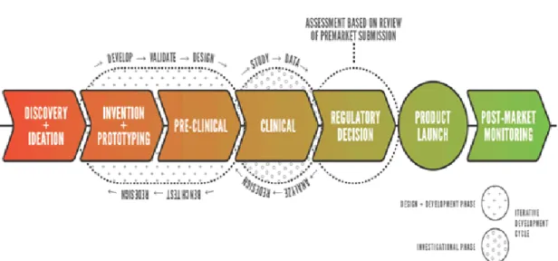
Figure 2.1 The Medical Device Development Pathway(CDRH Innovation Initiative, 2011)
In the medical device development pathway (Figure 2.1), the first step towards bringing a product to market is discovery and ideation. The regulatory process affects a significant portion of the device development pathway and should accommodate the iterative, cyclical nature of device design and development. At ForSight Laboratories, the focus is to achieve proof of concept through research and development of a product. One of the first hurdles of the development pathway begins with proof of concept. A good proof of concept should ideally be very cheap and easy to manufacture while sufficiently solving the problem at hand. The cost of the product is one factor that will determine the viability of the product and if it will move into the next stages of development.
8
matrix requires a delicate blend of the starting materials in order to achieve a homogenous formulation with a desired physical properties for ease of handling. Molding of the formulation is achieved by using a mold milled in a computer numerical controlled (CNC) machine and filled through a transfer press tailored to achieve an optimal fill. In order to finalize the product, the molded segments must be assembled. Assembly requires the use of an optical microscope and soldering iron to build the final ocular insert. Washing treats the product in order to reduce its bio burden and leads to a product with the desired release rate profile. Packaging and sterilization are necessary steps to finalize the product packaging prior to use.
Throughout the process, quality control maintains that the process and system under which all changes are done by maintaining a quality document system where everything is properly documented according to FDA compliance standards. Failure to adhere to quality control standards may result in failing FDA approval.
2.2. Formulation of a Drug Polymer Matrix
Silicone was chosen as a material to be used for sustained delivery of an
9
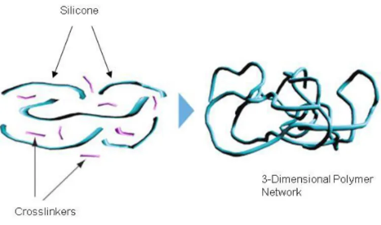
catalyzed silicone system from our sourced supplier was selected for formulating sustained release products (Figure 2.2).
Figure 2.2 Silicone Cross-Linking (DOW Corning, 2013)
During the early stage of product development, a 7% drug loaded matrix
produced the desired sustained release rate. The 7% drug-matrix was formulated using proprietary methods. Over time, a higher dosage with a longer release rate profile was desired. With the higher dosage form, a new formulation was developed since direct scaling up of the 7% formulation was not feasible.
The matrix approach was chosen over a reservoir approach for formulating the API into the silicone mainly due to the ease of manufacturing. The drug is mixed
10
2.3. Molding
Initially, molds were produced in batches of 20 segments. Molding development investigated diameters as well as designs of the final product. As manufacturing was developed, a higher production rate was desired resulting in a 40-up mold capable of producing double the segments per transfer press cycle. The silicone segments were injection molded and cured at elevated temperature using quality control approved process instructions as guidance.
2.4. Assembly
After the silicone formulation is molded into segments, they must be assembled into the final product. For every ocular insert produced, two segments are needed. Assembly requires the proper training of operators in order to have a high degree of reproducibility. Manufacturing development introduced more automated aspects of the process; however, operators remained essential to producing a viable ocular insert (Figure 2.3).
11
2.5. Wash
Once the product is assembled, each insert is treated in order to produce a final product with the desired release rate profile. The development of the wash method was a large focus of the research and development phase. The ideal release rate has a zero-order profile over the length of time that drug is to be released. This is normally
achieved through a reservoir system where the reservoir constantly feeds drug through an inert shell to the media. The inert shell is necessary to act as a rate limiting gradient; otherwise a high burst of drug would be seen. Since the design of the product utilizes a drug matrix instead of a reservoir system, an initial burst of drug was unavoidable. In order to mitigate the burst, washing is necessary. It was found that washing in water at elevated temperature for several days was needed to achieve the desired release rate of API at early time periods.
2.6. Packaging and Sterilization
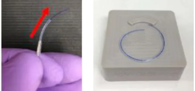
Each ocular insert was then packaged in a plastic tray and sealed in a foil pouch as shown in Figure 2.4. The packaged inserts were then sterilized via irradiation at a commercial e-beam facility at a sterilizing dose of 17.5 kGy.
12
3. Product Testing
Test methods were developed to assure that each insert is made as uniformly as possible. The two main modes of testing the chemistry of the product are through Content Uniformity and Assay and Impurities Determination, and Release Rate testing. Generic results in the form of high performance liquid chromatography (HPLC)
chromatograms are included to show what typical responses would be from the HPLC outputs. Actual results can be seen in the model development sections of this report.
3.1. Content Uniformity and Assay and Impurities Determination
3.1.1. Background
An HPLC analytical assay method for determining the API content and related impurities in Ocular Inserts was developed. The API and its impurities are analyzed by gradient reversed-phase HPLC with UV detection at 210nm.
3.1.2. Methods and Materials
13
3.1.3. Procedure
Mobile phase A for the HPLC was methanol/acetonitrile/water (10/10/80 v/v/v) with 0.05% H3PO4. The solution was mixed well prior to use.
Mobile phase B for the HPLC was methanol/acetonitrile/water (10/40/50 v/v/v) with 0.05% 85% H3PO4. The solution was mixed well prior to use.
Diluent Solution was methanol/acetonitrile/water (14/14/72 v/v/v. The solution was mixed well prior to use.
API reference standard was prepared at a concentration of ~150μg/mL. This was achieved by accurately weighting 7.50mg of API into a 50mL volumetric flask. The flask was filled up half way with diluent solution and diluted to the mark with water (the diluent amount is negligible and aids the dissolution of API in the solvent). Two standards were produced in the same fashion and labeled as “Working Standard” and “Check Standard.” The nominal concentrations of the standards were determined using the following equation:
Standard concentration (μg/mL) = 𝑊𝑠 𝑋 𝑃 𝑋 1000𝑉 ,
Where:
Ws = Recorded weight of API or Ref Standard (mg)
P = Purity of API based on Certificate of Analysis (CofA) for that particular lot
14
1000 = conversion factor for mg to μg
An LOQ (Limit of Quantitation) Standard was prepared at a concentration of ~0.15μg/mL. Into a 50mL volumetric flask, 50μL of API Stock Standard solution
(~150μg/mL) was pipetted. The flask was diluted with Diluent Solution and mixed well prior to use.
API resolution solutions of the impurities were prepared by first preparing stock solutions at a ~10μg/mL concentration by pipetting 10μL of API related impurity stock solutions into 10mL of 2-propanol (IPA) in a glass vial and mixed well prior to use. Resolution solutions were prepared by pipetting 40μL of the API related impurity solutions into an HPLC vial, 20μL of API stock standard solution (~150μL/mL) and 170μL of water into the same vial. The vial was mixed using a vortex shaker prior to use.
For content uniformity analysis, samples were prepared by placing ~70mg of cured drug-matrix into a 40mL glass vial referred to as the stock sample vial. To each vial, at least 20ml of dichloromethane (DCM) was added and the vial was sonicated for 100 minutes. All pieces of the drug-matrices were placed into 40mL glass vials already containing 5mL of DCM. The 40mL vials were sonicated for 10minutes and mixed for 5 seconds. The 5mL solutions were transferred into the 20mL solutions. The solutions were then dried at 37oC inside a fume hood by utilizing nitrogen gas to expedite the
15
was stored at 2-8oC when not in use. Final sample preparation involved diluting 1mL of
the sample solution with 2mL of water.
For assay and impurities, up to 10 individual samples were combined as a composite. Drug-matrices were cut into sizes which fit into a 40mL glass vial. At least 30mL of DCM was added into glass vials in order to completely immerse the pieces. The vials were capped tightly and sonicated for 100minutes. Sonication steps identical to content uniformity were followed (e.g. 30mL + 5mL DCM). Final solution was prepared by adding 1mL of the stock sample to a 10mL volumetric flask. The flask was filled with Diluent solution to volume.
The HPLC chromatographic conditions were a flow rate of 0.7mL per minute with an injection volume of 20μL, a column temperature of 50oC, a detection wavelength of
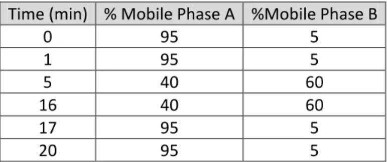
210nm, and a total run time of 20minutes. (Due to the use of a previously approved pharmaceutical, the known impurities generated have an absorbance at ~190nm. Since this wavelength tends to be very noisy when using a photodiode array detector, a more controllable wavelength was used). The gradient program is shown below in Table 3.1:
Table 3.1 Gradient Program of Mobile Phase Mixing. Time (min) % Mobile Phase A %Mobile Phase B
0 95 5
1 95 5
5 40 60
16 40 60
17 95 5
16
Chromatographic injection procedure followed equilibrating the HPLC system with mobile phase until a stable baseline is achieved. An injection of the working standard solution (~150μg/mL) may be done prior to starting the HPLC sequence to verify the retention time, USP tailing factor, and USP plate counts of the API peak. Mobile Phase A was injected at least once, followed by an injection of the diluent solution to ensure no interference with the API retention time. Sensitivity solution was injected to evaluate the method’s sensitivity.
System Suitability
System Suitability parameters outline acceptance criteria for acceptable data. First a blank is injected to ensure no peak interference. Five working standard injections are prepared and must have a relative standard deviation of the retention time and peak areas within ±2%. Next, there is a sensitivity - LOQ check where the signal-to-noise ratio for the API yielded from the LOQ Standard injection must be ≥ 10. A standard confirmation is then necessary and is done by evaluating the response factor from the check standard injection for the API; it must be within 98% - 102% of the average
response factor from the 5 replicate working standard injections. The percent difference
% Difference = Peak Area of Check Standard x Conc. of Working Standard
17
The tailing factors of the API peak from all working standard injections must be ≤ 2.The column efficiency is then checked by analyzing the column theoretical plate counts for the API peak from all the Working Standard injections and must be N ≥ 2000.The resolution factor for the API related impurity peaks relative to the API peak must be ≥ 1.5. The % difference of the peak areas for each bracketing standard must be ≤ 2% of the average peak area from the 5 replicate Working Standard injections.
Sample calculations
Measured API Content (µg)
Calculate the response factor for each Working Standard
RF = CStd AStd
Where:
RF = Response factor (concentration/peak area) Std
C = Expected API concentration in Working Standard (µg/mL)
Std
A = Peak area of API for Working Standard
The concentration of the sample solution is calculated from the average response factor of the standard curve.
Avg Smp
Smp A RF
C
Where:
Smp
C
= Measured API concentration in sample (µg/mL)
Smp
A
18 Avg
RF
= Average of the five response factors calculated for each Working Standard solution.
The total API content in µg is calculated by multiplying the sample concentration by the total volume of MeOH and dilution factor.
Measured API Content (µg) = CSmpVSmp DF
Where:
Smp
C
= Measured API concentration in sample (µg/mL)
Smp
V
= Total volume of MeOH (e.g., 25 or 35 mL) DF = Dilution factor (e.g., 3 or 10)
API Assay
The assay value for each content uniformity and assay sample is calculated by:
g LabelClaim g Content API Measured 100 =Assay
Where:
For pre-cured mix and cured segments: Label Claim = Weight of sample x %API Loading
For Ocular Inserts: Label Claim = as specified in Material Specification
Impurity Calculations
19
extraneous peaks that meet the aforementioned criteria in the assay chromatograms of the samples must be accounted for in the total peak area.
For each of the peaks detected, calculate its % purity by using the following formula:
Area Peak Total
Area Peak
Purity 100
% - % Impurities
For known impurities, a response factor was determined relative to the main API response factor and used to calculate % Impurities.
3.1.4. Results and Discussion
Typical chromatograms achieved when analyzing samples for content uniformity and assay and impurities are reproduced below.
20
Figure 3.2 Chromatogram of API Working Standard Solution (150 µg/mL)
21
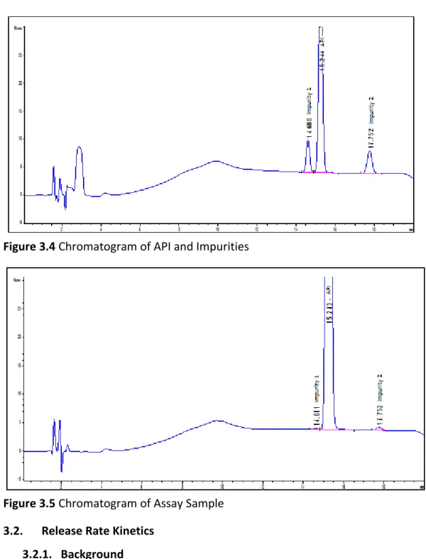
Figure 3.4 Chromatogram of API and Impurities
Figure 3.5 Chromatogram of Assay Sample 3.2. Release Rate Kinetics
3.2.1. Background
22
The purpose of this test method is to determine drug release rate (μg/day). The average daily drug release rate (μg/day) as well as the cumulative API released over an extended period will be determined by an in vitro test method developed by Forsight Vision5. API release is analyzed by reverse-phase HPLC with UV detection at 210 nm
3.2.2. Methods and Materials
An Agilent 1100 High Pressure Chromatographic System as described previously was used for sample analysis. Rainin Pipet-Lite series L-5000, L-1000, L-200, and L-20 pipets were used. A calibrated Mettler Toledo XS105 was used. An incubator set to 37oC
was used to store samples. Class A volumetric glassware was used. Final samples were stored in HPLC vials with PTFE/Silicone Pre-Slit Septa caps. Reagents used include HPLC grade water, HPLC grade acetonitrile, HPLC grade methanol, HPLC grade phosphoric acid, phosphate buffered saline (PBS) pH 7.4, sodium dodecyl sulfate (SDS), and reference standards of API were used.
3.2.3. Procedure
Release rate media was prepared by using 0.01M PBS solution with 0.05% SDS. Ocular inserts were weighed prior to use and placed in 15mL plastic vials. Into each plastic vial, 5mL of release media was added and the vials were capped. The start time was begun and considered as t=0. The vials were incubated at 37oC. At each of the
23
analysis. Analyzed samples were stored indefinitely at ambient temperatures. To the empty sample vials, and additional 5mL of release media was added. Incubation was continued at 37oC in an incubator until the next sampling time point. The amount of API
obtained was recorded. The drug release rate (μg/day) and the cumulative amount was calculated at each time point.
HPLC diluent and API standards were prepared as following the method outlined in the assay and impurities section of testing. The mobile phase was
methanol/acetonitrile/water (10/37/53, v/v/v) with 0.05% of 85% H3PO4. The increase in
polarity of the solvents relative to the Content Uniformity and Assay and Impurities Determination in section 3.1 is utilized in order to increase the throughput of any drug particles. The method utilized a 5 minute isocratic run time. Calculations of peak areas to release rates were carried out in the same fashion as section 3.1.
3.2.4. Results and Discussion
24
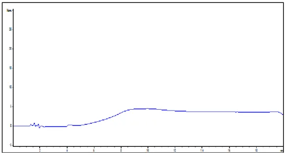
Figure 3.6 Chromatogram of Mobile Phase
c
25
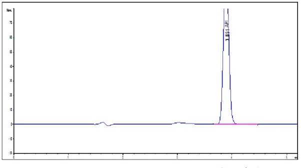
Figure 3.8 Chromatogram of API Working Standard Solution (15 µg/mL)
26
4. Product Development
After proof of concept has been established, and bench-top production has begun, the growth of the company occurs with pre-clinical investigations, regulatory filings, and clinical studies. During this stage, the goal for product development is to develop a product that can be made reproducibly with high quality so that pre-clinical and clinical evaluations generate valid results. While design changes fall under the realm of engineering, formulation and wash development fell under the realm of chemistry.
4.1. Formulation Development
Two formulation changes done to the product while scaling up batch production involved increasing the drug dose and changing the Durometer hardness of silicone. A higher drug loading was necessary in order to achieve a desired release rate. With the 7% formulation, the product was only capable of sustaining the desired release rate for 3 months. With higher drug loading, the product gives a higher release rate sustainable for up to 6 months. Saturation of the polymer matrix with the higher drug loading required different properties from the silicone in order to better contain the drug matrix.
4.1.1. Effect of Drug Loading on Release Rate
27
"initial burst" of drug, followed by a gradual decrease of release rate, eventually reaching a sustained steady-state level over time.
The drug release rate was found to increase with an increase in drug loading, as shown in Figure 4.1. This appears to indicate concentration gradient driven drug
diffusion across the silicone matrix
Figure 4.1 Release Rate of API as a Function of Drug Loading
28
Figure 4.2 Channel Formation in the Silicone Matrix Over Time (t)
The drug release rate continues to decline over time even though the estimated cumulative drug release over the time period studied is around 16% drug loading, indicating that the distance drug molecules need to travel from the inner bulk of the insert to the surface also likely plays a role in drug release rate.
Among all the different loadings in this silicone, 20% drug load appeared to meet the target drug release rate profile. However, the 20% API in these soft silicone inserts exhibited inconsistent mechanical properties and also appeared difficult to remove from the mold without breaking.
4.1.2. Effect of Different Silicones on the Release Rate
As an effort to improve the mechanical properties and manufacturability of the Ocular Inserts containing 20% drug load, a different silicone with the same cure
29
also easier to handle during manufacturing. Due to proprietary constraints, these two silicones will solely be referred to as 10A or 30A silicone.
The surface morphologies of the silicone segments prepared with 10A silicone vs. 30A silicones are shown in Figure 4.3. It appeared that the silicone segments made with the harder silicone have much smoother surfaces than those made with the softer silicone.
Figure 4.3 Surface Morphology of Silicone Segments Containing 20% API in Alternative Silicones
Representative drug release rates of silicone segments containing 20% API in each of the silicones are presented in Figure 4.4. Both the silicones appear to result in similar release rate profiles, suggesting that silicone physical property differences have little impact on drug release from the silicone matrix.
30
formulating higher drug load because of more consistent drug release rate, less surface deformities, improved mechanical properties and ease of manufacturability.
Figure 4.4 Release Rate of Ocular Insert Made with Silicones 10A and 30A 4.2. Effect of Wash on the Release Rate
Once molded and assembled, the insert is treated with a washing step. Different wash conditions produced different release rates. After the wash method was
established, modeling the release rate could be done in order to develop a more understandable product profile.
Washing procedures were studied with Ocular Inserts and Silicone Segments with the goal of reducing the initial burst and obtaining a zero-order release rate profile. The results of the development of washing studies are shown below.
4.2.1. Unwashed 7% API, 10A Silicone
31
Figure 4.5 Unwashed Release Rate
While this design demonstrated a potentially acceptable release rate profile, a lower initial release rate was desired. The goal of the following studies was to find the ideal washing conditions that would reduce the Day 1 burst and achieve a zero-order release rate profile.
4.2.2. 7% API/10A Silicone Matrix Water Washing Studies
32
Figure 4.6 Effect of Water Wash Length on Release Rate
33
Figure 4.7 Reductions in Burst due to IPA Wash Versus Water Wash
A further study was initiated to find the ideal water wash length that would reduce the initial burst to an appropriate level while allowing a reproducible manufacturing wash procedure with. Ocular Inserts in this study were made with 7% API in a 10A matrix.
The washing container used for all previous studies that utilized washing, either with IPA or water, was a large glass jar (unless otherwise specified, as for individually washed samples). Samples would be placed inside the same jar and the appropriate wash medium would be added.
34
set at 600C and 55 RPM for the duration of the wash. All Inserts were washed and then
irradiated.
Figure 4.8 Effect of Water Wash Length on Release Rate Using Washing Manufacturing Conditions
The data shown in Figure 4.8 demonstrates that both a 48 and 72 hour water wash reduce the initial burst from Ocular Inserts, while still maintaining a long term release rate profile comparable to unwashed samples. The 48 hour wash was chosen due to ease of manufacturing.
4.2.3. 20% API/30A Silicone Matrix Studies
35
to maintain the increased release rate of drug while keeping the initial drug burst from the device in an acceptable range.
Silicone Segments were made with 20% API loading in the 30A silicone matrix and were washed individually in glass vials containing water that were stored inside an oven set at 600C for 48 hours. Following the water wash, samples were washed with 70% IPA
for 15 minutes followed by a 1 minute 70% IPA rinse. Figure 4.9 shows the data for this study, and compares it with data from a previous 7% drug loading study with similar washing conditions.
Figure 4.9 20% Drug Load vs. 7% Drug Load Effect of Water Wash on Release Rate Comparison
36
Although the studies described above demonstrated that a 20% API loading provides a higher release rate profile than a 7% load, and a 48 hour wash is adequate to remove the initial burst, additional testing was done to confirm the effect of wash length on release rate.
Ocular Inserts made with 19% API (though deviation from 20% occurred during formulation, release rate profiles were deemed equivalent) in a 30A silicone matrix were washed individually in plastic jars containing water that were stored inside a shaking incubator set at 55 RPM and 600C. Samples were washed in water for different
lengths of time (6 hours, 24 hours, and 48 hours), and a 15 minute 70% IPA wash at room temperature followed the water wash.
Figure 4.10 Effect of Water Wash Length on Release Rate of 19% API loaded matrix
37
The long term release rate was not significantly affected however, as the release profiles for all samples began to converge around Day 30.
The release rate of the 48 hour wash sample was also very similar to the release rate seen from the 48 hour washed samples described above, indicating repeatability
The previous studies utilizing a 20% API loading demonstrated the feasibility of using an increased drug loading to increase the long term release rate. The next step was to show that the washing process was transferrable to a larger scale ‘manufacturing wash’ set-up.
Ocular Inserts made with 20% API in a 30A silicone matrix were washed in a custom Teflon tray that separated all Ocular Inserts. This tray was submerged into a polypropylene basin filled with water pre-heated to 600C, and the basin was held inside
a shaking incubator set at 50 RPM and 600C. The Ocular Inserts were washed for 48
38
Figure 4.11 Feasibility of the Manufacturing Washing Configuration for 20% API loaded product
The results shown in Figure 4.11 from the basin wash indicate that using the manufacturing washing configuration provided a release profile similar to that seen from samples washed individually. To confirm repeatability of the manufacturing wash process, 10 additional samples were tested (Figure 4.12).
39
Although the repeat samples average release rate profile was slightly higher, the basin washed and repeat basin washed samples release rate profiles fell within a relative standard deviation of 10%, as displayed in Figure 4.13 below:
Figure 4.13 20% Drug Load, 48 Hour Wash Comparison 4.2.4. Results and Discussion
40
Though the day1 burst was reduced to 68 µg/day, it was desired to reduce the burst still further. This was accomplished by washing Ocular Inserts in water at high
temperatures for an extended period of time, followed by a 15 minute 70% IPA wash. Washing in water at 600C for 48 hours reduced the burst from approximately 68 µg/day
to 18 µg/day, while maintaining the long term release rate profile.
Clinical data suggested that higher dosing was more desirable resulting in a 20% loaded product. Through testing, results indicated a long term release rate
approximately double that of the 7% loading was achievable. Burst moderation was achieved with identical water wash parameters used with the 7% loaded product. For example, Ocular Inserts washed inside a water filled basin placed inside a shaking incubator set at 600C for 48 hours produced a burst well under 60 µg/day while still
maintaining a release rate profile eluting over 8 µg/day by day 92.
41
wash time was recommended as a good overall balance for product performance and manufacturing efficiency.
Figure 4.14 Effect of Water Wash Time on Release Rate of 20% API loaded product
4.3. Manufacturing Reproducibility
42
Figure 4.15 Reproducibility for Three Different Batches
A 20% API in a 30A silicone formulation has been successfully developed. The formulation together with an appropriate manufacturing process has achieved
43
5. Understanding the Mechanisms of Release
5.1. Purpose
Mathematical modeling of the release rate of materials from polymer matrices is of particular interest to formulation chemists. One of the goal when developing any medical device is to develop the ability to control the properties of any system. Control of the formulation allows for optimization of the product; optimization allows for a tighter parameters during the manufacturability of the product. If the release rate of the device can be accurately predicted, it would show a certain degree of control over the system.
5.2. Controlled Release of Diffusion Based Processes
Diffusion is the transport of small molecules by random molecular motion of individual molecules from an area of high concentration to low concentration. Figure 5.1 below shows a typical schematic of this phenomenon analogous to the system
developed by ForSight Labs. Diffusion is a spontaneous process; it increases entropy, decreases Gibbs free energy, and is therefore isothermal dynamically favorably.
44
There are several factors that contribute to the transport process including the nature of the polymer, nature of cross links, effect of plasticizers, nature of penetrants, presence of fillers, effect of temperature, and presence of other variables that may be included in the system. The nature of the polymer includes the extent of unsaturation, degree of crystallinity, and the nature of substituents.
Different degrees of crosslinking density of the same polymer results in different physical properties such as glass transition temperatures (Tg). An increase in diffusion
coefficient is seen with decreasing Tg (George, 2001). Diffusivity has been shown to
decrease linearly with an increase in crosslink density until a maximum degree of crosslinking is reached resulting in a leveling off effect of diffusivity (Barrer, 1948). For
the same polymer with the same crosslink density, diffusion depends on the nature of crosslinks. In addition different solvent solutions of drug release affect the release rate differently. For example, benzene solutions swell more than corresponding bulk crosslinked networks having the same crosslink density which would decrease the rate of diffusivity (George, 2001).
Additional factors that contribute to transport processes are still significant, but fall outside the scope of the variables affecting the drug polymer matrix discussed in this report. For example, addition of plasticizers to a polymer results in an increased
segmental mobility which in turn usually increases penetrant transport, e.g. in the presence of solvents (George, 2001). The nature of the penetrant determines the
45
effects may increase or decrease the diffusivity of the molecule as well. The effects of all these variables that affect the release rate are captured mathematically in the diffusion coefficient of the model. The larger the diffusion coefficient, the higher the rate of release.
The aim of this project was to establish an understanding of the mechanisms relating solubility and transport in the polymer membrane to their molecular properties. The initial driving factor of the silicone-matrix drug delivery system developed at
ForSight is diffusion. However, as at some point in time, the mechanism of diffusion is overcome by the formation of channels due to the saturation of the matrix by the API. The kinetic model intends to develop a quantitative mechanism for determining the diffusion of API from the silicone matrix as well as the potential formation of a channel guided release mechanism.
The development of the model was necessitated by a need to interpret the response of release rate. The model was developed at a time when the focus of research and development was to optimize the washing parameters in order to determine the desired release rate profile. The main issue with release rate
46
development of the predictive model. This model minimized the time needed to understand the results.
The objectives of designing a model for controlled drug delivery systems are to:
1. Optimize the release rate development process 2. Elucidate the physical mechanisms of drug transport
3. Aid in the design new drug delivery systems based on release expressions 4. Predict drug release rates from and drug diffusion behavior through polymers
The purpose of mathematical models is to ultimately help optimize the design of a therapeutic device to yield information on the performance of the device as well as show the degree of accuracy through predictive models, thus avoiding excessive experimentation
Figure 5.2 Release Rate Profiles of 7% and 20% Drug Loading Used for Modeling Release rate profiles as seen in Figure 5.2 are broken down into several sections when applied for mathematical modeling. Release kinetics follow a well-defined
behavior: first a rapid initial release (termed the “burst”) followed by a slow near-zero
0 50 100 150 200 250 300
0 20 40 60 80 100 120 140 160 180
47
order release rate. The goal is to develop a model that both accurately models and has the capability of predictively determines release data.
5.3. A Background of Mathematical Modeling
5.3.1. Fick’s Law and its Analogous Counterparts
Adolf Fick was able to empirically derive an equation for diffusion in 1855. Inspired by many prominent scientists of his day, Fick’s laws of diffusion are analogous to the laws of transport and flow developed by Darcy (flow of liquid through a porous medium), Ohm (flow of current through two points) and Fourier (flow of heat). Their respective fundamental laws are described below.
Adolf Fick was the first to propose laws that govern the transport of mass through diffusive means. In addition to inspiration indirectly drawn from Ohm, Fourier, and Darcy, Fick was directly inspired by earlier experiments in diffusion by Thomas Graham. Although Thomas Graham was unsuccessful in his efforts, Fick was able to further Graham’s understanding and arrived at his successful laws of diffusion.
48
Though Fick is credited with development of the understanding of the
phenomena of diffusion, the evaluation of diffusion of solids was modeled by Noyes and Whitney in 1897 with the following equation:
𝑑𝑀
𝑑𝑡 = 𝐾𝑆 (𝐶𝑠− 𝐶𝑡)
where M is the mass transferred over time, t, by dissolution from the solid particle over a surface, S, under the driving force of the concentration difference (Cs – Ct) where Ct is
the concentration at time t andCs is the equilibrium solubility of the solute at the
experimental temperature. The rate of dissolution dM/dt is the amount dissolved per unit area per unit time and can generally be expressed in units g∙cm-2∙s-1.
To better fit more complicated systems, these fundamental models have been manipulated by the incorporation of appropriate variables. Additionally, the
development of these models has allowed for their application in other systems. For example, the diffusion mechanism which was first explained by Fick has since been modified by many scientists over the years into workable formulas for explaining the diffusion of pharmaceuticals. Though these models give credence to the Fick, they have been aptly renamed and are specific for their own systems. The proceeding sections gives insight into these models which have been applied to drug release from matrices.
5.3.2. Higuchi Model
49
developed into applications that incorporated multiple geometries and porosities. Several assumptions made by Higuchi include:
i. Initial drug concentration in the matrix is much higher than drug solubility; ii. Drug diffusion takes place only in one dimension (“edge effect must be
negligible”);
iii. Drug particles are much smaller than the channels through which they travel; iv. Matrix swelling and dissolution are negligible;
v. Drug diffusivity is constant;
vi. Perfect sink conditions are always attained in the release environment.
These same assumptions are the basis for the other mathematical models discussed in this report.
The basic model described by Higuchi is expressed by the equation:
𝑓𝑡= 𝑄 = 𝐴√𝐷(2𝐶 − 𝐶𝑠)𝐶𝑠𝐶𝑡
where ft is the cumulative fraction of drug in a given area at time t, Q is the amount of
drug released in time t per unit area A, C is the initial drug concentration, Cs is the drug solubility in the matrix media and D is the diffusion coefficient in the matrix substance.
The fundamental understanding of application of models on release kinetics was effectively established by Higuchi. Future model developers typically have their
50
5.3.3. Korsmeyer-Peppas Model (The Power Law)
In an effort to develop a more versatile kinetic model, Korsmeyer-Peppas proposed a model based on empirically derived data to describe drug release from polymeric systems in 1983 (Korsmeyer et al 1983):
𝑀𝑡
𝑀∞= 𝑘𝑡𝑛
where Mt/M∞ is a unit less cumulative fraction of drug released at time t, k is the
release rate constant and n is the release exponent. While modifications of the
Korsmeyer-Peppas model enables its application to various geometries, it is principally due to the position and simplicity of the n-variable that the model is typically applied to cylindrical shaped matrices when found in the most basic form.Depending on the value of the n-variable, the characteristics of the polymer matrix can be elucidated. A value of n= 0.5 indicates a Fickian diffusion drug transport mechanism. For cylindrical matrices, a value of n ≤ 0.45 is the most commonly found. A value of 0.45<n<0.89 corresponds to non-Fickian transport, n=0.89 for Case II relaxational transport, and n>0.89 for super relaxational transport. To determine the exponent n, drug release data in the initial range of Mt/M∞ < 0.6 are used to simulate the release profile. Release kinetics modeled
51
Table 5.1 Interpretation of Diffusional Release Mechanisms from Polymeric Films Release Exponent (n) Drug Transport Mechanism Rate as a Function of Time
0.5 Fickian diffusion t-0.5
0.45<n=0.89 Non-Fickian transport tn-1
0.89 Case II transport Zero Order Release Higher than 0.89 Super case II transport tn-1
5.3.4. Hixon-Crowell Model
In 1931, Hixson and Crowell recognized that a particle’s “regular” area is proportional to the cube root of its volume represented by the equation:
𝑊01/3− 𝑊𝑡1/3 = 𝜅𝑡
where W0 is the initial amount of drug in the pharmaceutical dosage form, Wt is the
remaining amount of drug in the pharmaceutical dosage form at time t and κ is a constant which incorporates the surface-volume relation.
This model is most useful in systems where there is a change in surface area and diameter of the pharmaceutical, such as in tablets. When this model is applied, release kinetics are typically viewed by plotting the cube root of drug percentage remaining in the matrix versus time. The model assumes that the diminishing dimensions of the pharmaceutical remain relative to each other (Dash 2012).
5.3.5. Weibull Model
52
function which was empirically derived and which has been adapted to the dissolution/release process.
The equation used when applying the Weibull model follows the form:
𝑀 = 𝑀0 [1 − (𝑒) (𝑡−𝑇)𝑏
𝑎 ]
where M is the amount of drug dissolved as a function of time t, M0 is the total amount
of drug being released, T accounts for the lag time measured as a result of the
dissolution process, a denotes a scale parameter that describes the time dependence, while b describes the shape of the dissolution curve progression. For b=1, the shape of the curve corresponds exactly to the shape of an exponential profile with the constant k=1/a resulting in the equation:
𝑀 = 𝑀0 [(1 − 𝑒)−𝑘(𝑡−𝑇)]
The shape of the curve becomes sigmoidal for values of b >1.
One application of the Weibull model is to determine the time when 50% (w/w) and 90% (w/w) of drug released from the formula is achieved:
𝑡(50% 𝑜𝑟 90%) = [−𝑎 𝑙𝑛
𝑀0− 𝑀 𝑀0 )
1 𝑏+ 𝑇]
53
5.3.6. Baker-Lonsdale Model
This model was first developed by Baker and Lonsdale in 1974 from the Higuchi model and was used to describe drug release from spherical matrices such as
microcapsules or microspheres. The generic equation of the model follows:
𝑓1 = 3
2[1 − (1 − 𝑀𝑡 𝑀∞)2/3]
𝑀𝑡 𝑀∞ = 𝑘𝑡
where k corresponds to the slope. Release kinetic data is most readily applied to
linearized data in the form [d(Mt/M∞ )]/dt with respect to the root of time inverse (Dash
2012).
5.3.7. Selection of an Appropriate Model
The most commonly applied models used to describe release phenomena are the Higuchi model, the Zero order model, the Weibull model, and the Korsmeyer-Peppas model. A summary of mathematical models can be seen in Table 5.2.
Table 5.2 Mathematical Models Used to Describe Drug Dissolution Curves. Zero Order Qt = Qo + Kot
First Order lnQt = lnQo + K1t
Second Order Qt/Q∞(Q∞--Qt ) Qo + Kot
Hixson-Crowell Qo1/3 - Qt1/3 =K1t
Weibull log[-ln(1-(Qt/Q∞))] = b X log t – log a
Higuchi Qt =KH√t
Baker-Lonsdale (3/2)[1-(-1(Qt/Q∞))2/3] – (Qt/Q∞) = Kt
KorsMeyer-Peppas Qt/Q∞ = Kk tn
Selection of an appropriate model can be quantified using the coefficient of determination, R2, which gives an appropriate fit of the model. For the determined
54 𝑅2 =𝑆𝑆𝑅
𝑆𝑆𝑇=
𝑆𝑆𝑅 𝑆𝑆𝑅 + 𝑆𝑆𝐸
SSR is the sum of squares due to regression determined by SSR = Σ(Ŷ-Ymean )2 . SSE is the
sum of squares due to error determined by SSE = Σ(Y-Ŷ)2 . SST is the total sum of
squares. Depicted in Figure 5.3, Ŷ is the predicted value for each Y. Since regressions are not exact fittings, there usually is some difference between each Y value and the fitted Y value. Ymean is the average of all empirically derived Y values.
Figure 5.3 Diagram for Determining Y-Values.
5.4. Model of 7% Drug Loading Washed in 70% IPA for 15min 5.4.1. Development of a Model
55
previous 30-days. In order to more accurately view the data, a necessary conversion to cumulative amount was needed.
5.4.2. Results and Discussion
In order to convert the release rate data to cumulative release, an accurate measure of the total drug content was needed. The assay data in Table 5.3 shows an average device weight in mg and amount of drug in micrograms and was obtained using the Content Uniformity and Assay and Impurities determination outlined in Section 3.1 of this report. An average recovery through HPLC analysis tended to yield 97% and was used as a conversion factor to aid modeling. Resulting data is shown in Tables 5.3 and 5.4.
Table 5.3 Assay Data From 7% Drug Loaded Device Wash Method
Device Weight (mg)
Amount of Drug in Device (µg)
97% recovery
70% IPA for 15min 64.372mg 4506.04 4370.86µg
Applying the assay data to the release rate yields the cumulative fraction of drug through the following equation:
𝑅𝑒𝑙𝑒𝑎𝑠𝑒 𝑅𝑎𝑡𝑒2− 𝑅𝑒𝑙𝑒𝑎𝑠𝑒 𝑅𝑎𝑡𝑒1
56
Table 5.4 Release Rate Data of 7% Device and Converted Cumulative Amounts Day Release Rate
(µg/day)
Cumulative
(µg) Cumulative Fraction
1 59.8 59.8 0.01
2 34.6 94.4 0.02
4 24.7 143.72 0.03
7 19.1 201.08 0.05
14 13.42 295.02 0.07
21 10.0 364.74 0.08
29 8.2 430.02 0.10
57 5.0 570.02 0.13
88 4.5 710.76 0.16
118 3.8 824.16 0.19
148 3.7 935.16 0.21
Figure 5.4 Cumulative Release Model Predicted Fit Versus Experimental of 7% Drug Loading Washed in 70% IPA for 15min
57
Figure 5.5 Release Rate: Model Developed Versus Experimental of 7% Drug Loading Washed in 70% IPA for 15min
The full data model fit in Figures 5.4 and 5.5 show how closely the
experimentally derived data follows power law functions and allowed for accurate use for predictive modeling. Because of the availability of data through day 148, predictive models could be instantly measured against real experimental data before being applied to new systems. Figure 5.6 shows the progression of the model as more time points became available relative to the empirical data.
58
Predictive models utilized a maximum of data through Day 28 since the majority of the release rate burst was diminished by this point and tended to show a near zero-order release rate past this point. Additionally, sampling time points were taken at Day 1, 2, 4, 7, 14, 21, and 28. Past Day 28, sampling time points were taken every 30 days. The time cost was greater than the marginal increase in model accuracy.
The predicted cumulative fractions were roughly 5% above the modeled fit by Day 150, the resulting release rate predictions were within 3µg for the Day 7 model and 1 µg for the Day 28 model. Since this difference was deemed within acceptable limits, the model was applied to other different wash conditions with different release rate profiles.
Figure 5.7 Release Rate: Prediction Intervals Versus Experimental of 7% Drug Loading Washed in 70% IPA for 15min
Graphically represented in Figure 5.7, a measurement of the fit of the models is tracked through analyzing their R2 values as summarized in Table 5.5. The Predictive
59
predicted fit approaches a 99% coefficient of determination. Calculation of the goodness measure of fit can be found in Appendix A.
Table 5.5 Measure of Fit of Model Based on Amount of Data
Data Range Model
R2 of Release Rate Model vs Empirical
Data Days 1-7 y = 0.0138x0.6219 0.976 Days 1-14 y = 0.014x0.6048 0.984
Days 1-21 y = 0.0141x0.593 0.986
Days 1-29 y = 0.0143x0.584 0.987
Days 1-148 y = 0.0152x0.538 0.976
Fickian Fit y = 0.0168x0.5 0.950
5.5. Model of 20% Drug Loading Washed in Water for 48hours at 60˚C 5.5.1. Development of a Model
The 20% Drug/Silicone matrix presented significant challenges. By increasing the drug loading in the polymer matrix, the characteristic behavior of the silicone was significantly changed. Previously, the 7% loaded device behaved under near ideal
diffusion based mechanisms. However, the 20% loaded matrix showed signs of a change in the mechanism of release due to the increase in drug loading. This change in the matrix was signaled during formulation developments where the 10A silicone was incapable of incorporating the higher drug load without affecting the physical properties of the silicone and required an alternative silicone in order to maintain structural
60
5.5.2. Results and Discussion
Table 5.6 Assay Data From 20% Drug Loaded Device Wash
Device Weight (mg)
Amount Drug (µg) 48hrs @ 60oC 70.56 12132.0
After wash, the amount of drug in each insert averaged 12mg (Table 5.6). The resulting release rate was once again converted to cumulative fractions shown in Table 5.7.
Table 5.7 Release Rate and Cumulative Release Data from 20% Drug Loading Day Release Rate
(µg/day)
Cumulative (µg)
Cumulative Fraction
1 36.68 36.68 0.003
2 24.42 61.11 0.005
4 22.06 105.22 0.009
7 21.21 168.86 0.014
14 18.01 294.95 0.024
22 15.18 416.37 0.034
28 13.93 499.95 0.041
60 11.35 863.25 0.071
91 9.54 1158.99 0.096
120 8.05 1275.77 0.105
150 6.86 1378.70 0.114
The final product had a significant drug load increase from 7% to 20% and was washed at 48hours at 60oC. The application of the normal model fit showed a cross
61
Figure 5.8 Cumulative Release Model Predicted Fit Versus Experimental of 20% Loading Washed in Water for 48hours at 60˚C
While the intersection was present when viewing the data as a cumulative fraction at Day 90, the only intersection for the release rate view was at Day 30 (Figure 5.9). This overlap was investigated and theorized as one of the main reasons for the differences caused between experimentally derived and modeled data.
62
The resulting predictive models deviated from experimental data by ~5% by Day 150 (Figure 5.14). This inaccuracy was investigated and attributed to a change in the release rate mechanism of the device that was not observed with the 7% loading.
Figure 5.10 Cumulative Release Model Predicted Fit Versus Experimental of 20% Loading Washed in Water for 48hours at 60˚C
The cumulative release view of data tended to highlight discrepancies. Resulting in a ~4µg difference between empirical and predicted data by Day 150 (Figure 5.15).
63
The resulting release kinetics fit of the 20% modeled fit with 48 hour wash at 60oC showed a roughly ~95% goodness of fit (Table 5.11). Calculation of the goodness
measure of fit can be found in Appendix C.
Table 5.11 Measure of Fit of Model Based on Variable Amounts of Data
Data Range Model
R2 of Release Rate
Model vs Empirical Data
Days 1-7 y = 0.003x0.7835 0.963
Days 1-14 y = 0.003x0.7935 0.942
Days 1-21 y = 0.003x0.7933 0.942
Days 1-28 y = 0.003x0.7919 0.946
64
6. Conclusions
Application of a direct Korsmeyer-Peppas fit as a prediction model resulted in a less than ideal fit of the actual release rates. During release rate determinations, it can be seen that regardless of the range of data used to forecast a predicted release rate, the predicted release rate values are significantly higher than the experimental values.
The first generation model involved fitting the known Korsmeyers-Peppas model. However an iteration of the model was necessary in order to achieve a higher degree of accuracy. Initially, this modification of the model was not necessary for the 7% Loading since application of the basic Korsmeyers-Peppas model showed a high degree of accuracy. For the higher 20% drug loading, a need for modification of the model was necessary, due to several competing theories as to why the power law fit no longer sufficed.
65
time resulting in a different contribution of each mechanism during different periods of time. For example, the release mechanism may initially have been purely due to Fickian diffusion. As drug diffused over time, channels were formed within the polymer matrix. The mechanism of channel formation in this case is analogous to non-Fickian transport since Fickian diffusion is based on “random walk” of molecules. When enough drug was removed from the surface, the main mode of release was through the channels,
resulting in a need to modify the power law fit in order to account for the mechanism changes. While The Korsmeyer-Peppas fit was ~95% accurate there was room to improve resulting in a second generation model.
This second generation model was a mixture of two models based off of the power law. The first model included the burst and the initial release time points. The second model took into account the later release profile. The final model was an
average of the two models and resulted in higher degree of accuracy. While the model is still in development, the initial developments are shown in Appendix D.
Process optimization was achieved by the development of a model. Reduction in R&D time constraints significantly reduced the real-time nature of data release.
Model developments in the future may be able to incorporate temperature, drug loading, and solution system variables. While it has proven difficult to correlate a
65
BIBLIOGRAPHY
Anderson DR. The Optic Nerve in Glaucoma. In: Tasman W, Jaeger EA, eds. Duane’s Ophthalmology. 15th ed. Philadelphia, Pa: Lippincott Williams & Wilkins; 2009:chap 48
Balcerzak, J., Mucha, M., “Analysis of Model Drug Release Kinetics from Complex Matrices of Polylactide-Chitosan,” Progress on Chemistry and Application of Chitin and Its Derivatives, 15, 2010, 117-126
Barrer, R.M., Chio, H., J Polym Sci, 1965; C10:111
Brazel, C., Peppas, N., “Modeling of Drug Release from Swellable Polymers,” European Journal of Pharmaceuticals and Biopharmaceutics, 49, 2000, 47-58
Carelli, V., Colo, G.C., Nannipieri, E., Serafini, M.F., “Journal of Controlled Release, 33, 1995, 153-162
CDRH Innovation Initiative, “Medical Device innovation Initiative White Paper”, About FDA, Feb 2011, <http://www.fda.gov/AboutFDA/CentersOffices/OfficeofMedical ProductsandTobacco/CDRH/CDRHInnovation/ucm242067.htm>
Costa, P., Manuel, Lobo, J.M.S., “ Modeling and Comparison of Dissolution Profiles,” European Journal of Pharmaceutical Sciences, 13, 2001, 123-133
Dash, S., Murthy, P.N., Nath, L., Chowdhury, P., “Kinetic Modeling on Drug Release from Controlled Drug Delivery Systems,” Acta Poloniae Pharmaceutica – Drug Release, 67, 2010, 217-223
DOWCorning, “Silicone Elastomers/Rubbers – Structure and Properties,”2013, <http://www.dowcorning.com/content/discover/discovertoolbox/forms-rubber-structure.aspx>
George, S., Thomas, S., “Transport Phenomena Through Polymeric Systems,” Prog. Polym. Sci., 26, 2001, 1985-1013
Giaconi JA, Law SK, Caprioli J. Primary Angle-Closure Glaucoma. In: Tasman W, Jaeger EA, eds. Duane’s Ophthalmology. 15th ed. Philadelphia, Pa: Lippincott Williams & Wilkins; 2009:chap 53
Grassi, M., Grassi, G., “Mathematical Modeling and Controlled Drug Delivery: Matrix Systems,” Current Drug Delivery, 2, 2005, 97-116