SOCIAL CLASS DISPARITIES IN PAIN: UNDERSTANDING THE ROLE OF SUBJECTIVE SOCIOECONOMIC STATUS AND HYPER-VIGILANCE TO THREATS
Jazmin Lati Brown-Iannuzzi
A dissertation submitted to the faculty at the University of North Carolina at Chapel Hill in partial fulfillment of the requirements for the degree of Doctor of Philosophy in the Department
of Psychology.
Chapel Hill 2015
ii © 2015
iii
ABSTRACT
Jazmin Lati Brown-Iannuzzi: Social class disparities in pain:
Understanding the role of subjective socioeconomic status and hyper-vigilance to threats (Under the direction of B. Keith Payne)
The relationship between wealth and health is strong: more wealth is associated with better health. Recently, researchers have turned to the importance of subjective socioeconomic status (sSES) in predicting health. Subjective SES is one’s perception of their social class rank as it compares to others. Subjective SES is often a better predictor of general health than are
objective measures of socioeconomic status (income and education). The relationship between sSES and pain, however, has received little attention. In this dissertation, I investigated the causal and correlational relationship between sSES and pain symptoms. In addition, I
iv
ACKNOWLEDGEMENTS
While at UNC, I once heard a professor say, “I am because we are.” This statement has truly resonated with me and defined my time at Carolina and beyond. Who I am as a researcher and as a person is because of some amazing individuals. I would like to take some time and thank these people. Although the words on this page can never truly express my gratitude, it is a start.
To my advisor Keith Payne, thank you for taking a chance on me. I showed up at your office seven years ago asking to be involved in research, and you welcomed me into your lab. You spent countless hours mentoring me, supporting me, and developing my academic skills. You led by example. Your dedication to science, precision in methods, and joy for discovery is truly inspiring.
To Sophie Trawalter, thank you for acting as a second mentor even after you went to UVA. I am so thankful for all of the time you spent mentoring me via skype, on email, during SPSP meetings, etc. You were always willing to squeeze me into your schedule, even when it was difficult for you. You didn’t need to spend so much time on me, and I will forever be grateful that you did.
v
To my fellow graduate students, thank you for the continued support. And, a special thanks to Kristjen Lundberg and Lindsay Kennedy. I would not have made it through this process without you two. You guys have been there through the ups and downs. I am a better person and scientist because of you both. Kristjen, we started this together, and I am so happy to be finishing this with you. I don’t know if you remember, but our third year at SPSP you saw Barb and her friend walking through the conference chatting and you said, “I hope that’s us one day. Best buds hanging out at a conference” I hope so too. It will be.
To my brother and dad, thanks for your continued support. To my mom, thank you for teaching me the meaning of hard work. You raised two kids on your own, often working more than one job. You were never given the opportunity to get a college degree, but you still instilled in me and my brother the importance of education. You have sacrificed and continue to sacrifice for my dream. I hope one day to provide for you the way you have provided for me.
vi
TABLE OF CONTENTS
LIST OF TABLES………...viii
LIST OF FIGURES………ix
CHAPTER 1: INTRODUTION……….……..1
The relationship between objective SES, subjective SES, and health………2
Is pain associated with sSES? ……….4
What mediates the relationship between sSES and pain? ………..5
Summary and hypotheses………..………10
CHAPTER 2: STUDY 1………12
Participants……….12
Design………12
Procedure………...13
CHAPTER 3: RESULTS STUDY 1……….17
Correlations between subjective SES, objective SES, and pain………17
Manipulation Check ……….….17
Did the manipulation of sSES cause difference in pain perception? ………18
Was measured sSES related to current pain perception? ……….19
Does hyper-vigilance mediate the relationship between measured and manipulated sSES and pain? ………..20
Threat Detection Task (TDT) ………...20
vii
State Anxiety……….23
CHAPTER 4: DISCUSSION STUDY 1………...…24
CHAPTER 5: STUDY 2………26
Participants……….26
Design………27
Procedure...………27
CHAPTER 6: RESULTS STUDY 2……….30
Correlations between subjective SES, objective SES, and pain………30
Manipulation Check………...30
Was manipulated sSES related to current pain perception? ……….31
Was measured sSES related to current pain perception? ……….…32
Does hyper-vigilance mediate the relationship between measured and manipulated sSES and pain? ...………...………33
Threat Detection Task (TDT). ………..33
Explicit Threat………...…35
State Anxiety………..…35
CHAPTER 7: DISCUSSION STUDY 2………...…38
CHAPTER 8: GENERAL DISCUSSION………39
Limitations and future directions………..…40
Conclusion………41
TABLES………...……42
FIGURES……….50
viii
LIST OF TABLES
Table
1. Study 1 correlations between subjective SES, objective SES, and pain……….42 2. Study 1 correlations between threat accuracy (d’) and response bias (c) for the
disease block and variables of interest……….43 3. Study 1 correlations between threat accuracy (d’) and response bias (c) for the
physical block and variables of interest………..44 4. Study 1 correlations between explicit physical and disease threat, state anxiety,
and variables of interest………..……….45 5. Study 2 correlations between subjective SES, objective SES, and pain………...….46 6. Study 2 correlations between threat accuracy (d’) and response bias (c) for the
disease block and variables of interest………...….…47 7. Study 2 correlations between threat accuracy (d’) and response bias (c) for the
physical block and variables of interest………...48 8. Study 2 correlations between explicit physical and disease threat, state anxiety, and
ix
LIST OF FIGURES
Figure 1 - Schematic representation of the threat detection task……….8 Figure 2 - Study 1: Mediation analyses demonstrating that state anxiety
partially mediated the relationship between measured sSES and pain…..………....50
Figure 3 - Study 2: Plotting the interaction between measured and manipulated sSES………....51 Figure 4 - Study 2: Plotting the interaction between state anxiety and
pain intensity over three time points…....………..52
Figure 5 - Study 2: Mediation analyses demonstrating that state anxiety
1
CHAPTER 1: INTRODUCTION
Income, education, and wealth are integrally linked with health. Individuals low in socioeconomic status (SES)—with little or no income, education, and/or wealth—have increased morbidity and premature mortality risk (Adler & Ostrov, 1999). This relationship between SES and health outcomes is robust across a wide range of physical and mental health symptoms. Low SES individuals have increased risk of aging diseases (e.g., cardiovascular disease, obesity, and diabetes), cancer (e.g., lung, testicular, and ovarian cancer), and mental health diseases (e.g., depression, generalized anxiety, and PTSD; for a review see Adler & Ostrove, 1999; Adler et al., 1994). Low SES individuals also report having greater pain intensity than do high SES
individuals (Thomtén, Soares, & Sundin, 2012). One reason for this relationship is presumably because low SES individuals lack basic resources, such as healthy food, clean living conditions, and/or access to health care. This lack of resources may predispose people to a variety of health problems that include painful symptoms. However, several lines of research suggest that above and beyond wealth, social and psychological factors also contribute to health.
One such factor is subjective SES (sSES)—the perception of one’s own social class rank as it compares to others. A growing body of research has found sSES to be a better predictor of health than is objective SES (oSES)– income, education, and wealth (e.g., Marmot et al., 1984; Singh-Manoux et al., 2005). In my own research, I have found that sSES mediates the
2
(Brown-Iannuzzi, Payne, Rini, DuHamel & Redd, 2014). However, the mechanism behind the relationship between sSES and health is poorly understood.
Some researchers theorize sSES is related to health via hyper-vigilance to environmental threats. That is, low sSES individuals are hyper-vigilant to environmental threats (Chen & Matthews, 2001; Kraus et al., 2012), which increases stress and, in turn, exacerbates negative health symptoms (Chen & Miller, 2013). Although some research has tested the link between SES and hyper-vigilance to threat (e.g., Chen & Matthews, 2001; Chan et al., 2011), and the link between hyper-vigilance to threat and health symptoms (e.g., McDermid et al., 1996), the full mediational model has yet to be systematically tested.
In this dissertation, I investigated the relationship between sSES and pain symptoms, controlling for oSES. In addition, I investigated a potential mediator between sSES and pain symptoms: hyper-vigilance to threat. Below, I detail the theoretical background which informed my dissertation studies. First, I will discuss the relationship between SES and health. Then I will discuss the potential relationship between sSES and pain. Finally, I will discuss the potential mediating role of hyper-vigilance.
The relationship between objective SES, subjective SES, and health
Objective SES is typically measured by averaging together income and education
(Krieger, Williams, & Moss, 1997; Gallo & Matthews, 2003). Objective SES has been associated with diverse health outcomes such as mental illness, aging diseases, cancer, and premature mortality (Adler & Ostrove, 1999). Originally, researchers believed that negative health
3
(Antonovsky, 1967). Using this logic, if people below the poverty line were simply given access to basic resources, then the association between oSES and health outcomes would disappear (Antonovsky, 1967). However, cross-sectional and longitudinal studies have found a linear relationship between oSES and health even among people who have access to basic resources. Because the relationship between oSES and health spans across the whole range of oSES, it is called the SES gradient.
The first landmark study which demonstrated the SES gradient was documented among a group of British civil servants in the Whitehall Study (Marmot et al., 1984). In this study, British civil servants ranging in occupational prestige were followed over 10 years. All of the
participants were employed, had incomes above the poverty line, and had access to health care. Despite uniform access to these basic resources, the civil servants exhibited a steep inverse relationship between occupational status (e.g., management vs. janitor) and health outcomes (heart disease, lung cancer, osteoarthritis, and premature death). Moreover, successive increases in job status were associated with increasingly better health outcomes. Even movement from the second highest to the highest status jobs was associated with improved health. Since this
landmark study, the SES gradient has been demonstrated in several countries including the United States (see Adler et al., 1994 for a review). Multiple studies have replicated the SES gradient demonstrating that as SES increases, morbidity and mortality decrease in a linear
fashion. This accumulation of evidence supporting the SES gradient spanning the whole range of SES suggests that factor other than access to basic resources may also influence health.
4
sSES are correlated (in my data the correlation across 8 data sets is r = .30, p <. 01), the
correlation is moderate, suggesting that the two constructs are related but distinct. Interestingly, the relationship between sSES and many health outcomes is stronger than the relationship between oSES and those health outcomes. A seminal study found that sSES was a better predictor of global health (including physical functioning, psychological functioning, social functioning, physical limitations, and emotional limitations) than was oSES. In addition, sSES was a better predictor of the decline in health over time than was oSES (Singh-Manoux, Marmot, & Adler, 2005). This dissertation will investigate whether sSES is a better predictor of pain than is oSES.
One unique aspect of investigating sSES (as opposed to oSES), is the ability to
manipulate this construct. Previous research has found that people’s perception of their social class rank can change depending on the social comparisons they are currently making (e.g., Piff et al., 2010; Kraus et al., 2012; Brown-Iannuzzi et al., 2014). For example, comparing yourself to Bill Gates may make you feel relatively poor, but comparing yourself to a homeless individual may make you feel relatively rich. This malleability of sSES allows researchers to utilize an experimental design to determine the causal pathway between sSES and behavioral and health outcomes. Thus, in the current research I will measure and manipulate sSES in hopes of determining the causal pathway between sSES and pain.
Is pain associated with sSES?
5
examining the differential impact of pain on life. This study asked participants to rate their pain on a scale from 1 (very mild) to 7 (very severe). Based on their responses to the pain scale, the researchers split the sample into seven subsamples (e.g., one sample who reported very mild pain, one sample who reported moderate pain, etc.). Then participants were asked the degree to which they felt “disabled through pain in carrying out necessary tasks.” Within each subsample, the researchers assessed whether oSES was associated with the degree to which people felt disabled by their pain. In every subsample, the results revealed that poor people reported feeling more disabled by their pain than did rich people. In fact, in some subsamples poor people were up to three times more likely to feel disabled by the pain than were rich people (Dorner et al., 2011). This suggests that even if the same level of pain is experienced, the impact of pain on daily life may be greater for low oSES individuals than for high oSES individuals.
Little research has investigated the relationship between sSES and pain until very recently. Among a large representative community sample collected in Scotland, the number of prescriptions filled for analgesic drugs was significantly higher for low sSES individuals than for high sSES individuals (Wakefield, Sani, Madhok, Norbury, & Dugard, 2015). Although this evidence does not directly link sSES to pain, it does infer the relationship via analgesic drug prescriptions. Importantly, in the current research I directly investigate the relationship between sSES (measured and manipulated) and pain.
What mediates the relationship between sSES and pain?
6
This state can be learned over time, or induced by motivated attention (see Crombez, Van
Damme, & Eccleston, 2005 for a review). Although at times helpful in identifying threats, hyper-vigilance may also lead to threat misidentification and unnecessary fear and avoidance of
situations. In fact, hyper-vigilance is associated with a number of anxiety disorders such as social phobia (Bögels & Mansel, 2004) and post-traumatic stress disorder (Dalgleish et al., 2001). Important to the current research, hyper-vigilance is also associated with increased pain intensity (McDermid, Rollman, & McCain, 1996).
A growing body of research suggests that hyper-vigilance not only increases pain intensity, but also lowers pain threshold and tolerance. The generalized hyper-vigilance hypothesis suggests that a person who is hyper-vigilant has increased attention devoted to potentially unpleasant stimuli. This attention in turn amplifies the experienced intensity of the stimulus (McDermid, Rollman, & McCain, 1996). Empirical research among fibromyalgia patients supports this hypothesis. The original study by McDermid and colleagues (1996) investigated whether hyper-vigilance (assessed using the Pennebaker Inventory of Limbic Languidness; PILL) was associated with pain tolerance, pain threshold, and noise tolerance among fibromyalgia patients, rheumatoid arthritis patients, and health controls. The findings revealed that fibromyalgia patients were significantly more hyper-vigilant than were rheumatoid arthritis patients and health controls. In addition, fibromyalgia patients had significantly reduced pain tolerance, pain threshold and noise tolerance than did rheumatoid arthritis and health
controls. Further research by Hollins and colleagues (2009) found that amplification in perceived pain intensity may occur at mildly painful levels of the noxious stimulus. The researchers
7
perceptual amplification of any potentially threatening stimulus. Thus, even low levels of a noxious stimulus may result in increased perceived pain.
Previous research has suggested that low oSES individuals are more likely than are high oSES individuals to be hyper-vigilant. For example, low (vs. high) oSES children were more likely to appraise an ambiguous event as threatening (Chen & Matthews, 2001). In addition, individuals who grew up in a low (vs. high) oSES family were more likely to misidentify a non-threatening object (e.g. a tool) as a non-threatening object (e.g., a gun) in a speeded visual perception task (Chan et al., 2011). Together, this suggests that low oSES individuals are more likely to misidentify innocuous events/objects as threatening.
Although hyper-vigilance may be associated with negative consequences, such as unnecessarily activating a stress response to an innocuous situation (Chan et al., 2011), it may still be useful for low SES individuals to be hyper-vigilant. One way to think about this is by analogy to a fire alarm. It is better for a fire alarm to have a “hair-trigger” for detecting fires even if that means the fire alarm will sometimes sound a false alarm. This is because if the fire alarm is less sensitive to fires, it could mean a small fire goes undetected until it grows into an
unmanageable fire. Thus, it is better to for the fire alarm to have more false alarms than to miss an actual fire. Relating this example to SES, it may be better for low SES individuals to have a “hair-trigger” at detecting threats. Low SES individuals have few resources with which to cope with threats. Thus, the negative consequences of falsely identifying an innocuous stimulus as a threat may be outweighed by the positive outcomes of avoiding all threats, especially for low SES individuals.
8
below). State anxiety refers to the extent to which people currently feel worried and tense and may reflect a state of extreme sensory sensitivity and increased readiness to respond to internal or external stimuli. Thus, state anxiety may be an appropriate way to assess hyper-vigilance.
In addition, I will assess hyper-vigilance by utilizing a modified Weapons Identification Task (Payne, 2001), which I call the Threat Detection Task (TDT). Originally, the Weapons Identification Task measured vigilance
to physical threats (e.g., guns) and social threats (e.g., Black Americans who are stereotyped as dangerous vs. White Americans who are stereotyped as relatively less dangerous). In the present work, I adapted this task to measure vigilance to disease and physical violence related threats. Specifically, in the adapted version of the task,
participants were presented with two images sequential. The first image, the prime, and the second image, the target, were either a neutral image or a threatening image. Participants were asked to ignore the prime and quickly determine whether there was threat present in the target image (see Figure 1 inset for a schematic representation of the task).
9
performance into accuracy (also called sensitivity or discriminability) and bias (also called criterion or threshold). Accuracy reflects the ability to distinguish between situations in which a true threat is present versus when it is absent. Bias reflects the tendency to judge that a threat is present, regardless of whether a true threat is present.
Vigilance to threats suggests a level of accuracy in correctly identifying an object as threatening. If low (subjective or objective) SES individuals are more vigilant to threats than are high SES individuals, then low SES individuals are better at accurately identifying
environmental threats. Some researchers have argued that low oSES individuals have greater accuracy in detecting threats than do high oSES individuals (e.g. Kraus et al., 2012) because they have more experience in doing so. Specifically, low (vs. high) oSES individuals are more likely to live in environments of physical violence and crime (e.g. Sampson, Raudenbush, & Earls, 1997), to be exposed to social threats such as stigmatization (e.g. Williams, 2007), and to have increased vulnerability to illness (Gallo & Matthews, 2003). In accordance with this theory, continual exposure to threats should train the threat detection system to accurately identify threats.
10
more likely to have a hyper-active threat detection system. To my knowledge, research has not disentangled vigilance from hyper-vigilance among a sample ranging in oSES (or sSES).
Using the vigilance and hyper-vigilance scores for each participant, I can test their association with oSES and sSES. Thus, I can determine whether low (subjective or objective) SES is associated with increased vigilance compared to high SES. If so, these findings would support the view that because low SES individuals have more experience detecting threats, they are more accurate than are high SES individuals (e.g., Kraus et al., 2012). I can also determine whether low (subjective or objective) SES is associated with increased hyper-vigilance compared to high SES. If so, these findings would support the view that because low SES individuals have a hyper-active threat detection system they are more likely to perceive threat in non-threatening situations than are high SES individuals (e.g., Chen & Matthews, 2001; Chan et al., 2011).
Predicting vigilance and hyper-vigilance from objective and sSES is important for three main reasons. First, this process can determine how resources and the perception of resources are related to threat detection. Second, I can test whether hyper-vigilance (or vigilance) mediates the relationship between sSES and pain. Third, the Threat Detection Task can determine whether SES predicts a differential reaction to a certain type of threat (e.g. physical violence).
Summary and hypotheses
11
12
CHAPTER 2: STUDY 1
The first study sought to determine whether high sSES, measured and manipulated, was associated with decreased hyper-vigilance to threats and decreased pain symptoms. This study was run online using a sample recruited from Amazon Mechanical Turk.
Participants
220 participants were recruited from Amazon Mechanical Turk. Due to attrition (N = 7) and failure to pass the attention check (N=19) the useable sample size was N = 194 (71 men). Because participants were not forced to complete all measures, the sample size varies across analyses. The average age of the sample was 37.74 years (SD = 11.71; ranging from 20 to 68 years). The majority of the sample was White or Caucasian (75%), but there were a few racial minority individuals as well (6% Black or African American, 5% Asian, 4% Hispanic, and 10% ‘Other’). The average income for the sample was $30,000 - $34,999 annually, and ranged from people who made less than $5,000 annually to people who made more than $175,000 annually. The majority of the sample had a 2-year college degree (N =57), with a sample range from less than a high school degree (N = 1) to a graduate degree (N = 2). All participants were
compensated $0.45 for their time.
Design
13
Procedure
First, participants were asked to complete some questions on their spending habits. These questions included items assessing income and spending habits, as well as demographic
information, financial conscientiousness, and personality traits. After participants completed this measure, they received feedback in the form of a “Comparative Discretionary Income (CDI) Index,” which determined participants’ relative amount of discretionary income compared to their peers. Regardless of how participants completed the measure, they were randomly assigned to receive feedback that they had either relatively more or less discretionary income than their peers (Callan, Shead, & Olson, 2011). After participants received this feedback, they were asked to complete the MacAthur Ladder. This measure asked participants to think of a “ladder as representing where people stand in the United States. At the top of the ladder are the people who are the best off—those who have the most money, the most education, and the most respected jobs. At the bottom are the people who are the worst off—who have the least money, least education, and the least respected jobs or no job.” Then participants were asked to determine where they stand relative to other people in the United States. This measure was used as a manipulation check.
14
The prime was presented for 100ms, followed by a brief blank screen (75ms), then the target was presented for 100ms, and finally a mask covered up the target image and remained on the screen until participants responded. Participants were given 600ms to respond. If the
participant took longer than 600ms to respond, a warning mask appeared on the screen for
1000ms which read, “Please try to respond faster!” Both the prime (the first image) and the target (the second image) were randomly pulled from a list of neutral and threatening images.
There were two blocks in this task: the physical violence block and the disease contagion block. In the physical violence block, participants were asked to determine whether the target represented a threat of physical violence. In the disease contagion block, participants were asked to determine whether the target represented a threat of disease contagion. Within each block, there were 80 trials: 20 trials where both the prime and target images were threatening, 20 trials where the prime was threatening and the target was neutral, 20 trials were the prime was neutral and the target was threatening, and 20 trials where both the prime and target were neutral. Trials were randomly presented within block, and blocks were randomly presented to avoid order effects (for scoring of the TDT see Appendix A).
15
with the following statements: (1) “There are many dangerous infectious diseases in our society which can attack anyone;” (2) “It seems that every year there are more and more infectious diseases which threaten everyone.”
Then participants were asked to complete a measure of current physical symptoms: a modified version of the Pennebaker Inventory of Limbic Languidness (Pennebaker, 1982). In this version, participants were presented with several symptoms (such as chest pains, sore muscles, headache, etc.) and were asked the extent to which they were currently feeling these symptoms (1 = Not at all; 5 = Extremely). Scores were averaged across all of the items to create one index which represented current physical symptoms (called mPILL; Cronbach’s α = .95).
Participants also completed questions which assessed current pain. One item asked participants to indicate which areas on their body they are currently experiencing pain (e.g., neck, back, arms, etc.). Another item assessed the intensity of the current pain (0 =No pain; 10 = Pain as bad as you can imagine).The last scale (3 items) measured the degree to which pain was disrupting current functioning, such as one’s ability to concentrate, one’s mood, one’s ability to complete the survey (0 =Pain is not interfering; 10 = Pain is completely interfering). All of these measures were standardized and then averaged together to create one index which represented current level of pain (called pain; Cronbach’s α = .81).
After participants completed the pain measures, they completed the state portion (20 questions) of the State Trait Anxiety Inventory (called State Anxiety; Cronbach’s α = .94;
Spielberger et al., 1983). These questions include items such as, “I feel calm” (reverse scored), “I am tense,” and “I am presently worrying over possible misfortunes.”
16
income, education, Mother’s Education, and Father’s Education). To measure sSES, participants completed two versions of the MacArthur Ladder (described above), and a sSES measure by Griskeviscious and colleagues (2011). The MacArthur Ladder was measured twice to assess two different relative status comparisons: (1) participants’ current standing relative to other people in the United States, and (2) their current standing relative to their peers. Three additional items were used to measure adult sSES (from Griskeviscious et al., 2011). An example item is: “Now, I have enough money to buy things I want” (1 = strongly disagree; 7 = strongly agree). I
17
CHAPTER 3: RESULTS STUDY 1
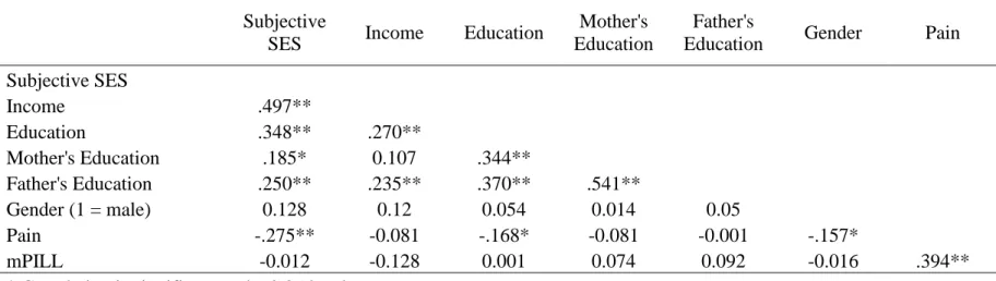
Correlations between subjective SES, objective SES, and pain
First, as an initial investigation of the data I tested the correlations among measured sSES, oSES, and the pain measures (see Table1). I hypothesized that measured sSES would be significantly associated with current pain. Consistent with this hypothesis, measured sSES was associated with current pain such that participants who self-reported being high (vs. low) in sSES reported less current pain, r (177) = -.28, p < .001. Neither manipulated nor measured sSES were associated with the modified PILL, r (178) = -.09, p = .23; r (178) = -.01, p = .87 respectively. This suggests that perceptions of socioeconomic status may be important for predicting current pain experiences but not current physical symptoms more broadly.
I also hypothesized that oSES (income, education, and parental education) would be significantly associated with the pain measures. Contrary to this hypothesis, income was not associated with current pain (r = -.08, p = .28), but more personal education was associated with less current pain (r = -.17, p = .03). Objective indicators of SES were also not associated with the modified PILL (p’s > .09).
Manipulation Check
18
Inconsistent with this hypothesis, there was no difference between condition, F(184) = 2.29, p = .76; MHigh SES = 4.49 (1.77), MLow SES = 4.42 (1.51)1. Upon further inspection, I found that sSES, race, gender, and age did not moderate these findings. There was a marginally significant three-way interaction between condition, sSES, and gender; b = .56, p = .08. Probing of this interaction revealed that men high in sSES placed themselves higher on the ladder when in the high sSES condition than in the low sSES condition. However, for everyone else, condition did not influence people’s placement on the ladder. Given the failed manipulation check, I cautiously interpret the following findings.
Did the manipulation of sSES cause differences in pain perception?
My primary hypothesis was that manipulated sSES would be associated with differences in current pain perception. In order to test this hypothesis, I ran an independent samples t-test. Consistent with my hypothesis, participants who were randomly assigned to learn they had relatively more wealth than similar others also reported fewer current pain symptoms (M = -.16, SD = .78) than participants who were randomly assigned to learn they had relatively less wealth than similar others (M = .15, SD = .92), t(172) = 2.39, p = .02. This finding was not moderated by sSES, gender, or the three-way interaction between condition, sSES, and gender, p’s > .20.
In order to understand exactly which measures of current pain symptoms were being influenced by condition, I broke apart the pain measure into body pain (the number of areas the participant reported currently having pain), pain intensity (a one item measure which assessed the amount of pain the participant was currently experiencing), and the extent to which pain is currently disrupting the participant’s mood, ability to concentrate, and ability to complete the survey. The results revealed that participants who were randomly assigned to learn they had
1 I ran this study 3 times using three different sSES manipulations. In every study, the manipulation check revealed
19
relatively more wealth than similar others reported fewer body areas of pain (M = .60, SD = 1.28) than participants who were randomly assigned to learn they had relatively less wealth than similar others (M = 1.31, SD = 1.2), t(155.71) = 2.91, p = .004. In addition, participants who were randomly assigned to learn they had relatively more wealth than similar others also reported marginally less pain intensity (M = 1.10, SD = 1.94) than participants who were randomly assigned to learn they had relatively less wealth than similar others (M = 1.69, SD = 2.1), t(176) = 1.92, p = .057. Finally, participants who were randomly assigned to learn they had relatively more wealth than similar others also reported pain was disrupting their current mood marginally less (M = .68, SD = 1.65) than participants who were randomly assigned to learn they had relatively less wealth than similar others (M = 1.20, SD = 2.05), t(169.56) = 1.87, p = .064. Condition did not affect the extent to which pain was disrupting the participants’ ability to complete the survey or concentrate, p’s > .35. The primary hypothesis was generally supported: participants reported greater pain in the low sSES condition than in the high sSES condition.
Was measured sSES related to current pain perception?
I also investigated whether measured sSES was uniquely associated with current pain. In a two-step OLS regression, I first regressed pain onto income, parental education, and gender. I control for gender in these analyses because some research suggests that women tend to report greater pain than do men (Berkley, 1997). In the second step, I added sSES as a predictor. Consistent with my hypothesis, high sSES participants reported less current pain than low sSES participants, b = -.29, p = .001 ∆R2 = .05. No other control variables were significant predictors of pain.
20
body areas with pain than low sSES participants, b = -.55, p = .001 ∆R2 = .05. In addition, high sSES participants reported less pain intensity than low sSES participants, b = -.56, p = .009 ∆R2 = .04. Low sSES participants reported pain was disrupting their mood more than high sSES participants, b = -.62, p = .001 ∆R2 = .06. sSES did not affect the extent to which pain was disrupting the participants’ ability to complete the survey or concentrate, p’s > .30. The primary hypothesis was generally supported: low sSES participants reported greater pain than did high sSES participants.
Does hyper-vigilance mediate the relationship between measured and manipulated sSES and pain?
In addition to my primary hypothesis, I also investigated a potential mechanism: vigilance/hyper-vigilance to threat. Three measures assessed hyper-vigilance. I individually detail the results of these three measures below.
Threat Detection Task (TDT).
21
participants were less accurate at detecting the threatening target when the prime was threatening (M =1.53, SD = 1.19) than when the prime was neutral (M = 1.79, SD = 1.11), F (1, 146) = 6.90, p = .01. Together, this suggests that when participants were primed with threatening images (compared to non-threatening images), their ability to accurately determine whether the target was threatening or non-threatening was diminished.
I also investigated whether participants’ response bias (c) – the extent to which
participants tended think all stimuli were threatening—was influenced by the prime photos (for scoring see Appendix A). I calculated the response bias score for neutral (cneutral)and threatening
(cthreat)primes for each block of trials. Then, within each block, I ran a repeated measures
ANOVA with prime type (threatening or non-threatening) as the within subjects factor. For the disease threat block, there was a significant effect of prime such that participants had a greater bias to respond ‘threat’ when the prime was threatening (M = -.53, SD = .83) than when the prime was neutral (M = .01, SD = .69), F (1, 194) = 60.89, p < .001. In addition, for the physical violence threat block, there was a significant effect of prime such that participants had a greater bias to respond ‘threat’ when the prime was threatening (M = -.65, SD = .83) than when the prime was neutral (M = -.03, SD = .57), F (1, 146) = 87.77, p < .001. Together, these findings suggest that when participants were primed with threatening images (compared to
non-threatening images), they were more likely to identify the target as non-threatening. Overall, these data suggest the TDT is a valid measure of threat detection.
22
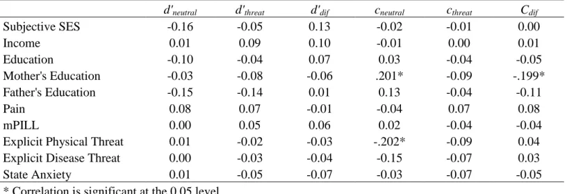
subtracted the d’neutral score from the d’threat score within each block to create a d’dif score. In addition, I created a cdif score within each block using the same method. Then I investigated whether condition influenced these scores. There was no significant difference between conditions on any of the accuracy or bias scores, p’s > .15. I also correlated all of these scores with sSES, oSES, and pain. For the disease block, there were no significant correlations between accuracy or response bias with sSES or pain (see Table 2 for correlations). However, there was a marginally significant correlation between measured sSES and d’neutral such that high sSES individuals were worse at detecting threat when the prime was neutral than low sSES
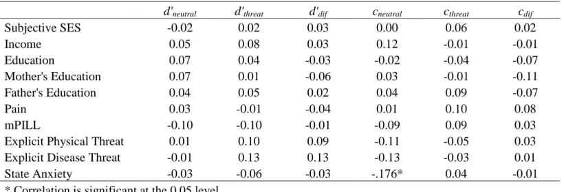
individuals, r(138) = -.16, p = .06. For the physical block, there were no significant correlations between accuracy or response bias with sSES or pain (see Table 3 for correlations). Together, these data are inconsistent with my hypothesis thus suggesting that accuracy and response bias may not be a mechanism by which sSES is associated with pain.
Explicit Threat.
I hypothesized that higher sSES, measured and manipulated, would be associated with a reduced perception that the world is violent place (explicit physical threat), and a reduced
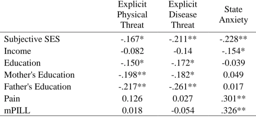
perception the world is full of contagious diseases (explicit disease threat). I investigated whether condition influenced explicit threat. There was no significant difference between conditions on either explicit physical or disease threat, p’s > .11. Explicit physical and disease threats were related to measured sSES such that high sSES individuals reported less explicit threat, r (178) = -.17, p = .03, r(178) = -.21, p =.005 respectively.To investigate the unique relationship between explicit threat and sSES, I ran a regression predicting explicit threat from sSES, income,
23 State Anxiety.
Finally, I assessed the relationship between sSES and state anxiety. I hypothesized that higher sSES, measured and manipulated, would be associated with a less state anxiety. There was no relationship between the state anxiety and condition, p’s > .15. There was a relationship between state anxiety and measured sSES such that high sSES individuals reported less state anxiety than low sSES individuls. To investigate the unique relationship between state anxiety and sSES, I ran a regression predicting state anxiety from sSES, income, education, parental education, and gender. None of the control variables were significant predictors of state anxiety. Consistent with my hypothesis, sSES uniquely predicted state anxiety such that high sSES
individuals reported less state anxiety than did low sSES individuals, b = -.14, p = .01, ∆R2 = .03. This pattern of results suggests that state anxiety may mediate the relationship between sSES and pain. To test this mediational pattern, I used the bootstrapping method recommended by Preacher and Hayes (2008). In addition, I controlled for income, education, parental
24
CHAPTER 4: DISCUSSION STUDY 1
The results of study 1 provided some encouraging evidence for my primary hypothesis. Manipulated sSES caused differences in current pain symptoms. Participants who were randomly assigned to the high sSES condition reported less current pain than did participants who were randomly assigned to the low sSES condition. In addition, measured sSES was associated with current pain such that high sSES participants reported less current pain than did low sSES participants. In addition, the data provided preliminary evidence that state anxiety mediates the relationship between measured sSES and pain.
Although these results are encouraging, there were several limitations to this study. First, it is unclear whether the manipulation of sSES was effective. Manipulated sSES did not reveal a significant difference on the manipulation check. Further inspection of the data suggests that the manipulation may have only worked for a subset of the sample, namely high sSES men.
However, the difference in pain by condition was not moderated by gender, sSES, or the three-way interaction. The manipulation may have led to an implicit change in psychological state which in turn influenced pain perception, but did not explicitly change ratings on the MacArthur Ladder. This suggests the manipulation was not robust enough to product an explicit change in sSES.
25
26
CHAPTER 5: STUDY 2
Study 2 sought to determine whether high sSES, measured and manipulated, was
associated with decreased pain intensity and increased pain tolerance. In addition, I investigated the mediating role of hyper-vigilance. This study was run at the University of North Carolina using a sample recruited from the Psychology 101 Participant Pool.
Participants
27
Design
Participants were randomly assigned to one of two sSES conditions. In the high sSES condition, participants were asked to consider a high anchor value before judging their own subjective SES. In the low sSES condition, participants were asked to consider a low anchor value. Much research on the anchoring effect (Tversky & Kahneman, 1974) suggests that when people consider a specific numeric value before making a numeric judgment, their judgment tends to be biased toward that “anchor” value. Thus, we expected participants who considered a high anchor value to rate their own sSES higher than participants who considered a low anchor value.
The classic anchoring effect shows that the act of considering the high or low anchor value shifts subsequent judgments in the direction of the anchor (Tversky & Kahneman, 1974). Later research suggested that a key mechanism driving the anchoring effect is that people tend to selectively retrieve similarities between the anchor value and the judgment to be made (see Mussweiler, Englich, & Strack, 2004 for a review). We asked participants to generate similarities between themselves and the anchor group to maximize the impact of the anchoring manipulation, and to reduce the likelihood that participants judged themselves as different from the anchors (i.e., a contrast effect) by thinking about how they are different from the anchor groups.
Procedure
28
the least money, the least education, and the least respected jobs or no job. In the high sSES condition, there was a red X placed near the top of the ladder (on the 13th rung out of 15 rungs). Participants were asked to think of 2 reasons why they were similar to people at this rung of the ladder, and then to judge whether their own status was higher or lower than this value. In the low sSES condition, there was a red X placed near the bottom of the ladder (on the 3rd rung out of 15 rungs). Participants were asked to think of 2 reasons why they were similar to people at this rung of the ladder and to indicate whether their own status was higher or lower than this value. After participants made these judgments, they were asked to determine where they thought they actually stood on the ladder. Next, participants were asked to complete the cold pressor task (Silverthorn & Michael, 2013). Participants were encouraged to take their hand out of the water whenever the pain approached a level of pain they no longer wished to tolerate. The water was set to 5° Celsius, and an upper limit was set at 2 minutes. While the participant’s hand was in the water, the participant was asked to report her pain intensity at 10 seconds, 30 seconds, and right before she pulled her hand out of the water. In addition, the experimenter recorded how long the participant kept her hand in the water using a stop watch as a measure of pain tolerance.
Next, participants were asked to complete the explicit threat questionnaires, state anxiety questionnaire, and Threat Detection Task. These were the same measures as used in study 1.
Finally, participants completed objective and sSES measures. For objective SES, participants completed a measure of familial annual income, and parental education (Mother’s Education and Father’s Education). To measure sSES, participants completed the same
29
30
CHAPTER 6: RESULTS STUDY 2
Correlations between subjective SES, objective SES, and pain
First, as an initial investigation of the data I tested the correlations among measured sSES, oSES, pain intensity at three time points, and pain tolerance (see Table 5). I hypothesized that sSES would be significantly associated with pain intensity and pain tolerance. Consistent with this hypothesis, measured sSES was significantly associated with pain tolerance such that high sSES individuals kept their hand in the water for longer than low sSES individuals, r(108) = .24, p = .01.However, sSES was not associated with pain intensity at any of the time points. This suggests that perceptions of socioeconomic status may be important for predicting pain tolerance, but not pain intensity.
I also hypothesized that oSES (income and parental education) would be significantly associated with the pain measures. Interestingly, only mother’s education was associated with pain tolerance such that higher mother’s education was associated with greater pain tolerance, r(108) = .24, p = .01. No other oSES measures were associated with pain intensity or pain tolerance.
Manipulation Check
31
condition placed themselves significantly higher on the ladder (M = 8.06, SD = 1.89) than participants in the low sSES condition (M = 7.06, SD = 2.07),t(103) = -2.59, p = .01.
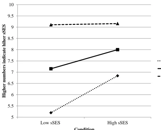
I also investigated whether gender, race, and sSES moderated these findings. The results revealed that gender and race did not moderate the findings. However, there was a marginally significant two-way interaction between condition and sSES, b = -.79, p = .07 (see Figure 3 for a graph of the interaction). Probing of this interaction that for people high in sSES (1 SD above the mean), condition did not change where people placed themselves on the ladder, t = .10, p = .92. However, for people at or below the mean of sSES, people in the high sSES condition placed themselves significantly higher on the ladder than people low in sSES; tMean = 2.68, p = .009, t1SD
below mean = 3.05, p = .003. This suggests that the manipulation may have only worked for people
at or below the mean of measured sSES. Therefore, I will cautiously interpret the following findings.
Was manipulated sSES related to current pain perception?
My primary hypothesis was that manipulated sSES was associated with differences in current pain perception. In order to test this hypothesis, I ran an independent samples t-test on the measure of pain tolerance. Inconsistent with my hypothesis, people in the high sSES condition did not keep their hands in the water longer (M = 69.53, SD = 37.69) than people in the low sSES condition (M = 73.60, SD = 37.62), t(108) = .57, p = .57. I also investigated whether gender, race, and sSES moderated the finding and I found that none of these variables did moderate the finding. This suggests that manipulated sSES did not change pain tolerance.
32
data. Random intercepts allows every participant’s initial pain intensity rating to have a unique intercept, and random slopes allows every participant to have a unique trajectory in pain intensity over time. Inconsistent with my hypothesis, there was no main effect of condition which means pain intensity at time one did not differ as a function of condition, b = .41, p = .29. In addition, there was no interaction between condition and time which means people’s pain intensity trajectory did not differ as a function of condition, b = -.06, p = .75. I also investigated whether gender, race, and sSES moderated these findings and I found that none of these variables did moderate the findings. This suggests that manipulated sSES did not change pain intensity.
Was measured sSES related to current pain perception?
I also investigated whether measured sSES was associated with current pain perception in the cold pressor task. First, I investigated whether sSES was associated with pain tolerance. In a two-step OLS regression, I first regressed the amount of time the participant kept his/her hand in the water onto income, parental education, and gender. In the second step, I added sSES as a predictor. Consistent with my hypothesis, high sSES participants kept their hand in the water longer than low sSES participants, b = .30, p = .03 ∆R2 = .04. Interestingly, income was a significant predictor of pain in the opposite direction: low income participants kept their hand in the water longer than high income participants, b = -.23, p = .04. No other control variables were significant predictors of pain tolerance.
33
b =-.18, p = .54. In addition, there was no interaction between sSES and time which means people’s pain intensity trajectory did not differ as a function of sSES, b = -.10, p = .43.
Does hyper-vigilance mediate the relationship between measured and manipulated sSES and pain?
Threat Detection Task (TDT).
First, I investigated the validity of the TDT in this sample. I investigated whether participants’ accuracy (d’)—the extent to which participants could distinguish threat from noise— was influenced by the prime photos For the disease threat block, there was a marginally significant effect of prime such that participants were more inaccurate at detecting the
threatening target when the prime was threatening (M =.50, SD = .58) than when the prime was neutral (M = .62, SD = .52), F (1, 55) = 3.56, p = .06. For the physical violence threat block, the effect was not significant, F (1, 62) = 2.27, p = .14. This suggests that the prime may alter participants’ ability to determine whether the target was threatening or non-threatening was diminished.2
Next, I investigated whether participants’ response bias(c)– the extent to which
participants tended think all stimuli are threatening—was influenced by the prime photos. For the disease threat block, there was a significant effect of prime such that participants had a greater bias to respond targets were threatening when the prime was threatening (M = -.34, SD = .46) than when the prime was neutral (M = -.02, SD = .54), F (1, 106) = 46.19, p < .001. In addition, for the physical violence threat block, there was a significant effect of prime such that
participants had a greater bias to respond targets were threatening when the prime was
threatening (M = -.40, SD = .44) than when the prime was neutral (M = -.13, SD = .50), F (1,
2 The small sample size may be the reason these results were not significant. For some reason, the computer
34
106) = 38.70, p < .001. Together, this suggests that when participants were primed with
threatening images (compared to non-threatening images), they were more likely to identify the target as threatening. Overall, these data confirm the validity of this task to measure threat detection.
Finally, I investigated whether d’ and c were related to sSES and pain. I hypothesized that low sSES individuals may be better at detecting threat (greater d’ scores) and more likely to say all stimuli are threatening (more negative c scores) than high sSES individuals. In order to investigate this hypothesis, I subtracted the d’neutral score from the d’threat score within each block to create a d’dif score. In addition, I created a cdif score within each block using the same method. Then I correlated all of these scores with sSES, oSES, and pain. For the disease block, there were no significant correlations between accuracy or response bias with sSES or pain (see Table 6 for correlations). However, there was a marginally significant correlation between condition and
cneutralsuch that high sSES individuals were more likely to think the target was threatening when
the prime was neutral, r(106) = -.18, p = .07. In addition, there was a marginally significant correlation between condition and cdif such that high sSES individuals were more likely to think the target was not a threat than low sSES individuals, r(106)= .19, p = .054.
For the physical block, d’neutral and d’threatwere not associated with measured or
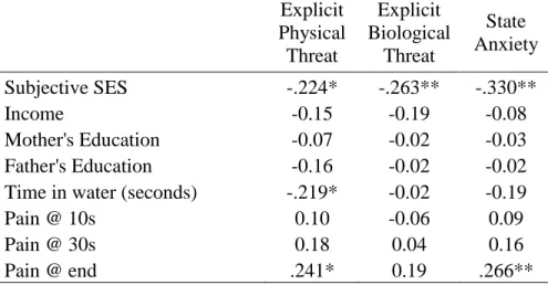
35 Explicit Threat.
In addition, I assessed the relationship between sSES and explicit threat. I hypothesized that high sSES, measured and manipulated, would be associated with the perception that the world is safe. There was no relationship between the explicit threat variables and condition. Explicit physical and disease threat were related to measured sSES such that high sSES individuals reported less explicit threat, r’s < -.22, p’s < .05 (see Table 8). To investigate the unique relationship between explicit threat and sSES, I ran a regression predicting explicit threat from sSES, income, education, parental education, and gender. In this model, sSES was a
marginally significant predictor of explicit physical threat (b = -.30, p = .054), and explicit disease threat (b = -.28, p = .09). In addition, explicit physical threat was marginally associated with time 2 pain intensity and significantly associated with time 3 pain intensity. To investigate whether explicit physical threat uniquely predicted pain intensity over time, I used a multilevel model with random intercepts and random slopes. There was no main effect of explicit physical threat which means that explicit threat did not predict people’s pain intensity rating at time 1, b = .03, p = .88. In addition, there was not a significant relationship between explicit physical threat and people’s pain intensity trajectory, b = .14, p = .10. Thus, it does not seem that explicit physical threat mediates the relationship between sSES and pain intensity.
State Anxiety.
36
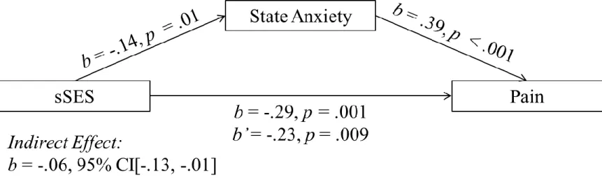
than low sSES individuals, r(109) = -.33, p < .001 (see Table 8). To investigate the unique relationship between state anxiety and sSES, I ran a regression predicting state anxiety from sSES, income, parental education, and gender. None of the control variables were significant predictors of state anxiety. Consistent with my hypothesis, sSES uniquely predicted state anxiety such that high sSES individuals reported less state anxiety than low sSES individuals, b = -.47, p < .01, ∆R2 = .09. I also investigated whether state anxiety predicted pain tolerance. I ran a
regression predicting state anxiety from income, parental education and gender and found that state anxiety was a marginally significant predictor of pain tolerance, b = -.18, p = .07. Although this pattern suggests that state anxiety may mediate the relationship between sSES and pain tolerance, the indirect effect was not significant, b = .06, 95% CI[-.02, .17].
In addition, I investigated whether pain intensity differed by measured state anxiety. I ran a multilevel model (MLM) with random intercepts and random slopes. In this model, I controlled for participants’ sSES, gender, familial income, and parental education. There was no main effect of state anxiety which means that state anxiety did not predict people’s pain intensity rating at time 1, b = -.03, p = .89. However, there was a marginally significant relationship between state anxiety and time which means people’s pain intensity trajectory did differ over time as a function of state anxiety, b = .17, p = .06. To probe this interaction, I investigated the effect of state
anxiety on the trajectory of pain intensity at one standard deviation above and below the mean of state anxiety. For both one standard deviation above and below the mean of state anxiety, the slope of the trajectory was significantly different from zero, t (105) = 14.78, p < .001 and t(107) = 12.16, p < .001. Although the slope did not become non-significant, they were slightly
37
38
CHAPTER 7: DISCUSSION STUDY 2
The results of study 2 were partially encouraging of my hypothesis. I hypothesized that high sSES, measured and manipulated, would be associated with decreased pain intensity and increased pain tolerance to the same noxious stimulus (cold water). I found that measured sSES was associated with pain tolerance such that high sSES individuals had greater pain tolerance. However, I did not find that measured sSES was associated with pain intensity. In addition, manipulated sSES was not associated with either pain intensity or pain tolerance. The lack of association between manipulated sSES and pain may be due to a failure of the manipulation or an incorrect hypothesis.
39
CHAPTER 8: GENERAL DISCUSSION
Across two studies, I investigated whether sSES caused differences in pain symptoms. I hypothesized that when people felt relatively wealthy they would report less current pain
symptoms than when they felt relatively poor. This hypothesis was made based on the perceived resources perspective. That is, when people feel they do not have many financial resources, a painful event may feel more extreme because they do not have the resources to overcome the challenge. However, when people feel flush with resources, a painful event may feel relatively minor because they do have the resources to overcome the challenge.
Overall, these studies were partially encouraging of my primary hypothesis. In study 1, manipulated sSES caused differences in current pain symptoms. People who were randomly assigned to the high sSES condition reported fewer current pain symptoms than did people who were randomly assigned to the low sSES condition. In study 2, however, I did not find that manipulated sSES caused differences in either pain intensity or pain tolerance in response to the cold pressor task. However, in both studies, I measured sSES and found that measured sSES was associated with current pain symptoms. This suggests that sSES is related to current pain
symptoms and may cause differences in current pain symptoms.
40
experience noxious stimuli more intensely than do high sSES individuals. In both studies I measured hyper-vigilance using a threat detection task and a measure of state anxiety. I found that neither vigilance nor hyper-vigilance as measured by the TDT was associated with either measured or manipulated sSES or pain. However, I did find evidence that state anxiety partially mediates the relationship between measured sSES and pain. In study 1, state anxiety partially mediated the relationship between measured sSES and current pain. In study 2, state anxiety partially mediated the relationship between measured sSES and pain intensity. This suggests that hyper-vigilance, as measured by state anxiety, may be the psychological mechanism which links sSES to current pain symptoms.
Limitations and future directions
Although there were promising findings in these two studies, both studies suffer from limitations. In both studies, it was unclear whether the manipulation of sSES was effective. The lack of a robust manipulation eliminates my ability to determine a causal pathway between sSES and pain. Future research should investigate creating a more robust manipulation. In addition, future research should use a longitudinal approach to measuring sSES and pain to investigate whether sSES predicts pain intensity over time. Moreover, longitudinal designs could investigate whether changes in sSES over time predict subsequent changes in pain over time. Longitudinal designs and more robust experimental manipulations of sSES can help determine a causal pathway between sSES and pain.
41
field (the first paper by Piff and colleagues appeared in 2010). Furthermore, no published papers have investigated the relationship between manipulated sSES and pain. Therefore, future
research should increase the sample size for appropriately powered analyses.
Finally, future research should investigate whether sSES is associated with pain
symptoms in chronic pain patients. Some research suggests that low sSES people are more likely to fill prescriptions for analgesic drugs than are high sSES individuals (Wakefield, Sani,
Madhok, Norbury, & Dugard, 2015). However, research has not directly assessed whether sSES is associated with pain among this extremely vulnerable population. If so, this would suggest that sSES may not only cause every day aches and pains, but also may cause a downward spiral which results in chronic pain. Understanding the full extent to which sSES may cause pain may help direct interventions to reduce SES-related pain disparities.
Conclusion
42
TABLE 1: Study 1 correlations between subjective SES, objective SES, and pain
Subjective
SES Income Education
Mother's Education
Father's
Education Gender Pain Subjective SES
Income .497**
Education .348** .270**
Mother's Education .185* 0.107 .344**
Father's Education .250** .235** .370** .541**
Gender (1 = male) 0.128 0.12 0.054 0.014 0.05
Pain -.275** -0.081 -.168* -0.081 -0.001 -.157*
mPILL -0.012 -0.128 0.001 0.074 0.092 -0.016 .394**
* Correlation is significant at the 0.05 level ** Correlation is significant at the 0.01 level
43
TABLE 2: Study 1 correlations between threat accuracy (d’) and response bias (c) for the disease block and variables of
interest.
d'neutral d'threat d'dif cneutral cthreat Cdif
Subjective SES -0.16 -0.05 0.13 -0.02 -0.01 0.00
Income 0.01 0.09 0.10 -0.01 0.00 0.01
Education -0.10 -0.04 0.07 0.03 -0.04 -0.05
Mother's Education -0.03 -0.08 -0.06 .201* -0.09 -.199*
Father's Education -0.15 -0.14 0.01 0.13 -0.04 -0.11
Pain 0.08 0.07 -0.01 -0.04 0.07 0.08
mPILL 0.00 0.05 0.06 0.02 -0.04 -0.04
Explicit Physical Threat 0.01 -0.02 -0.03 -.202* -0.09 0.04
Explicit Disease Threat 0.00 -0.03 -0.04 -0.15 -0.07 0.03
State Anxiety 0.01 -0.05 -0.07 -0.03 -0.07 -0.05
* Correlation is significant at the 0.05 level
Note: d’neutral represents the accuracy score when the prime is neutral. d’threat represents the accuracy score when the prime is threatening. d'dif = d’threat - d’neutral. cneutral represents the response bias score when the prime is neutral. cthreat represents the response bias score when the prime is threatening. Cdif = cneutral - cthreat.
44
TABLE 3: Study 1 correlations between threat accuracy (d’) and response bias (c)
for the physical block and variables of interest.
d'neutral d'threat d'dif cneutral cthreat cdif
Subjective SES -0.02 0.02 0.03 0.00 0.06 0.02
Income 0.05 0.08 0.03 0.12 -0.01 -0.01
Education 0.07 0.04 -0.03 -0.02 -0.04 -0.07
Mother's Education 0.07 0.01 -0.06 0.03 -0.01 -0.11
Father's Education 0.04 0.05 0.02 0.04 0.09 -0.07
Pain 0.03 -0.01 -0.04 0.01 0.10 0.08
mPILL -0.10 -0.10 -0.01 -0.09 0.09 0.03
Explicit Physical Threat 0.01 0.10 0.09 -0.11 -0.05 0.03
Explicit Disease Threat -0.01 0.13 0.13 -0.13 -0.03 0.01
State Anxiety -0.03 -0.06 -0.03 -.176* 0.04 -0.01
* Correlation is significant at the 0.05 level
Note: d’neutral represents the accuracy score when the prime is neutral. d’threat represents the accuracy score when the prime is threatening. d'dif = d’threat - d’neutral. cneutral represents the response bias score when the prime is neutral. cthreat represents the response bias score when the prime is threatening. Cdif = cneutral - cthreat.
45
TABLE 4: Study 1 correlations between explicit physical and disease threat, state anxiety, and variables of interest.
Explicit Physical Threat
Explicit Disease Threat
State Anxiety
Subjective SES -.167* -.211** -.228**
Income -0.082 -0.14 -.154*
Education -.150* -.172* -0.039
Mother's Education -.198** -.182* 0.049 Father's Education -.217** -.261** 0.017
Pain 0.126 0.027 .301**
mPILL 0.018 -0.054 .326**
* Correlation is significant at the 0.05 level ** Correlation is significant at the 0.01 level
46
TABLE 5: Study 2 correlations between subjective SES, objective SES, and pain
Subjective
SES Income
Mother's Education
Father's
Education Gender
Pain @ 10s
Pain @ 30s
Pain @ end
Income .383**
Mother's Education .245* .417**
Father's Education .253** .491** .601**
Gender (1 = male) -.221* -0.074 -0.048 -0.024
Pain @ 10s -0.085 0.098 -0.137 -0.056 0.188
Pain @ 30s -0.009 0.129 0.002 0.066 0.141 .852**
Pain @ end -0.144 0.013 -0.017 0.028 0.162 .557** .761**
Time in water (seconds) .242* 0.005 .241* 0.181 -0.18 -.577** -.619** -.426** *Correlation is significant at the 0.05 level
** Correlation is significant at the 0.01 level
47
TABLE 6: Study 2 correlations between threat accuracy (d’) and response bias (c)
for the disease block and variables of interest.
d'neutral d'threat d'dif cneutral cthreat cdif
Subjective SES 0.06 0.15 0.11 0.00 -0.05 -0.04
Income -0.16 -0.08 0.08 0.15 0.08 -0.09
Mother's Education -0.12 -0.06 0.06 0.16 -0.04 -.222*
Father's Education 0.13 0.07 -0.05 0.18 0.03 -0.17
Time in water (seconds) .293* .307* 0.05 .238* 0.04 -.226*
Pain @ 10s -0.13 -0.17 -0.07 -0.10 0.01 0.13
Pain @ 30s 0.07 -0.03 -0.12 -0.12 0.02 0.16
Pain @ end 0.13 0.04 -0.09 -0.15 -0.09 0.08
* Correlation is significant at the 0.05 level
Note: d’neutral represents the accuracy score when the prime is neutral. d’threat represents the accuracy score when the prime is threatening. d'dif = d’threat - d’neutral. cneutral represents the response bias score when the prime is neutral. cthreat represents the response bias score when the prime is threatening. Cdif = cneutral - cthreat.
48
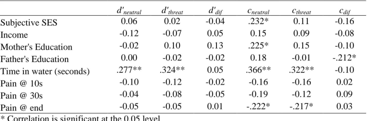
TABLE 7: Study 2 correlations between threat accuracy (d’) and response bias (c)
for the physical block and variables of interest.
d'neutral d'threat d'dif cneutral cthreat cdif
Subjective SES 0.06 0.02 -0.04 .232* 0.11 -0.16
Income -0.12 -0.07 0.05 0.15 0.09 -0.08
Mother's Education -0.02 0.10 0.13 .225* 0.15 -0.10
Father's Education 0.00 -0.02 -0.02 0.18 -0.01 -.212*
Time in water (seconds) .277** .324** 0.05 .366** .322** -0.10
Pain @ 10s -0.10 -0.12 -0.02 -0.16 -0.16 0.02
Pain @ 30s -0.04 -0.08 -0.05 -0.19 -0.12 0.09
Pain @ end -0.05 -0.05 0.01 -.222* -.217* 0.03
* Correlation is significant at the 0.05 level ** Correlation is significant at the 0.01 level
Note: d’neutral represents the accuracy score when the prime is neutral. d’threat represents the accuracy score when the prime is threatening. d'dif = d’threat - d’neutral. cneutral represents the response bias score when the prime is neutral. cthreat represents the response bias score when the prime is threatening. Cdif = cneutral - cthreat.