EXPOSURE TO URBANIZATION AND ITS LONGITUDINAL ASSOCIATION WITH BLOOD AND PULSE PRESSURE IN ADULT FILIPINO WOMEN
Alberto Vargas
A thesis submitted to the faculty at the University of North Carolina at Chapel Hill in partial fulfillment of the requirements for the degree of Master of Science in the Department of Nutrition in the Gillings
School of Global Public Health.
Chapel Hill 2017
Approved by: Linda S. Adair
ABSTRACT
Alberto Vargas: Exposure to Urbanization and its Longitudinal Association with Blood and Pulse Pressure in Adult Filipino Women
(Under the direction of Linda Adair)
Urbanization may adversely affect blood (BP) and pulse pressures (PP) as individuals migrate or
as their surroundings urbanize. We determined how urbanicity (UI) is associated with BP and PP in adult
women of the Cebu Longitudinal Health and Nutrition Survey (CLHNS) from 1998-2012.
We identified participants (N=2107) as movers and non-movers. The former moved between communities between survey years (1998, 2002, 2005, and 2012). We estimated mixed-effects longitudinal regression models of the change in UI-change in SBP, DBP, and PP relationships.
Movers’ UI increased more than non-movers’ throughout follow-up. Change in UI effected change in SBP, DBP, and PP differently according to previous UI. Moving effected change in SBP, DBP, but not PP, differently according to previous UI.
TABLE OF CONTENTS
LIST OF TABLES ... v
LIST OF FIGURES ... vi
LIST OF ABBREVIATIONS ... vii
CHAPTER 1-URBANICITY AND BLOOD PRESSURE IN THE PHILIPPINES ... 1
Background ... 1
Methods ... 3
Study Variables ... 3
Statistical Analyses ... 6
Results ... 9
Changes and Secular trends in BP, PP, and UI ... 11
Change in BP models ... 11
Medication model ... 22
Mortality Outcome Models ... 23
CHAPTER 2-DISCUSSION AND SYNTHESIS ... 24
Overview of Major Findings ... 24
Comparison with Previous Literature ... 25
Limitations and Strengths ... 27
Public Health Implications and Conclusions ... 28
APPENDIX 1: ADDITIONAL RESULTS ... 30
LIST OF TABLES
TABLE 1 - Demographic characteristics of a longitudinal cohort of eligible
participants in the Philippines in 1998 ... 10
TABLE 2 - Final Change in BP by change in UI model results output ... 21
TABLE 3 - Full medication model results output ... 22
TABLE 4 – Mortality outcome model results ... 23
SUPPLEMENTAL TABLE 1 - Correlation matrix of household asset variables included in household wealth score ... 30
SUPPLEMENTAL TABLE 1.1 - Notation key for SUPPLEMENTAL TABLES 2-5 ... 31
SUPPLEMENTAL TABLE 2 - Characteristics of a Longitudinal Cohort of Eligible Adult Filipino Women Participants from 1998-2012 ... 32
SUPPLEMENTAL TABLE 3 - Characteristics of a Longitudinal Cohort of Eligible Adult Filipino Women Participants by Moving Status 1998-2012 ... 33
SUPPLEMENTAL TABLE 4 - Longitudinal Characteristics of Non-Movers by Direction of Urbanization from 1998-2012 ... 34
LIST OF FIGURES
FIGURE 1 - Directed Acyclic Graph of the Relationship between change
change in UI and change in BP and PP ... 8 FIGURE 2 - Mean systolic and diastolic blood pressure of CLHNS
women by survey year ... 12 FIGURE 3 - Observed secular trends in SBP and DBP from 1998-2012
stratified by baseline age groups ... 13
FIGURE 4 - Observed median Urbanicity Index* by survey year, moving
patterns, and direction of urbanization ... 14 FIGURE 5 - Predicted change in SBP by change in UI across previous UI ... 16 FIGURE 6 - Predicted change in SBP by change in UI and age ... 16
FIGURE 7 - Predicted change in DBP by change in UI across previous UI
Adult Filipino Women Participants from 1998-2012 ... 18 FIGURE 8 - Predicted change in DBP by change in UI across age
Adult Filipino Women Participants by Moving Status 1998-2012 ... 18 FIGURE 9 - Predicted change in PP by change in UI previous UI
Direction of Urbanization from 1998-2012 ... 20 FIGURE 10 - Predicted change in PP by change in UI across age
Direction of Urbanization from 1998-2012 ... 20 SUPPLEMENTAL FIGURE 1 - Observed secular trends in SBP and DBP from 1998-2012 by
LIST OF ABBREVIATIONS
24-HR 24-hour Recall
BMI Body-Mass Index
BP Blood Pressure
CLHNS Cebu Longitudinal Health and Nutrition Survey
CM Cardiometabolic
CMD Cardiometabolic Disease
CVD Cardiovascular Disease
DAG Directed Acyclic Graph
DBP Diastolic Blood Pressure
FCT Food Composition Table
IWI International Wealth Index
LMIC Low and Middle Income Countries
NNS National Nutrition Survey
PP Pulse Pressure
SBP Systolic Blood Pressure
SES Socioeconomic Status
UI Urbanicity Index
CHAPTER 1: URBANICITY AND BLOOD PRESSURE IN THE PHILIPPINES
Background
Living in urban environments may adversely affect health by promoting poor dietary habits,
physical inactivity, and cigarette smoking in low and middle income countries (LMICs). Together, these
behaviors contribute to the burden of chronic diseases such as obesity, diabetes, and hypertension,
increasingly seen in LMICs undergoing the nutrition transition. On the other hand, urbanization may also
improve health by increasing availability and accessibility of health care, and by providing centralized
services such as piped water. While the higher socioeconomic status (SES) associated with greater
urbanization may partially mitigate the burden of obesity and hypertension, obesity is still more
prevalent among the most affluent in LMICs, but the burden is now shifting to the poorest.
The Philippines exemplifies many of the changes associated with the nutrition transition1, including
increasing rates of obesity and cardiovascular diseases. Previous research from the Cebu Longitudinal
Health and Nutrition Survey (CLHNS) found that the risk for hypertension is twice as high among
overweight compared to normal or underweight weight Filipino women2. In addition, the risk for stage II
hypertension (Systolic Blood Pressure >= 160 or DBP >=100) is more than twice as high among those
with abdominal obesity (Waist-to-hip Ratio >0.85) compared with those with normal abdominal
adiposity2. Trends in blood pressure status among Filipino adults aged >20y from the nationally
representative Philippine National Nutrition Survey (NNS) show that hypertension has been prevalent in
1 in 5 adults since 2003.3, 4
Hypertension may be prevalent in both the affluent and the poor and in urban and rural communities. In
hypertension among higher SES, more urban populations, but excessive sodium consumption associated
with poverty diets may dominate among the rural poor.
Dietary and environmental exposures associated with urbanization and modernization may be
key risk factors in the development and progression of hypertension as individuals are exposed to urban
environments due to abrupt migration into more urban places or as their surroundings urbanize over
time. Yet, we know little about how exposure to urban environments impacts CM health in
populations with different history of exposure to urban environments. Specifically, it is not yet clear how exposure to urban environments relates to SBP and DBP separately despite the current medically relevant individual SBP and DBP cutoff values used to define different BP status categories.
Furthermore, the relationship between urbanicity and pulse pressure (PP) has never been explored
despite this parameter being considered as a significant independent predictor of stroke and myocardial
infarction among middle-aged and older adults.5-8
The current study aims to determine how exposure to urban environments is associated with systolic and diastolic blood pressure in a cohort of adult Filipino women from the CLHNS. This cohort is
important to study due to higher CMD risk found in Asian populations at lower BMI levels compared
with Caucasians39. The Philippines is an important site for this research due to its rapid urbanization and
socioeconomic development since the advent of the CLHNS in 1983.
To address current gaps in the literature, we will (1) describe CLHNS participants’ exposure to urbanicity and their patterns of SBP, DBP, and PP across four survey rounds (1998, 2002, 2005, and
2012), (2) classify exposure to urbanicity into two mutually exclusive groups comprised of those who
moved to different communities between survey rounds and those who remained in the same
communities between survey rounds, and (3) estimate the longitudinal association between change in
determine whether abrupt changes related to moving to a different community vs gradual change
related to increasing urbanization in situ relate differently to BP.
Methods
Data were derived from the CLHNS, a community based survey that initially enrolled 3,327 pregnant women from 33 randomly selected urban and rural barangays (administrative units, that are communities in urban areas or villages in rural areas) of Metro Cebu. The CLHNS has followed these women since 198331. The study includes high quality information on barangay characteristics that
describe population size and density, communication and health services, metropolitan transportation,
and types and number of markets for >150 barangays measured over time. BP and waist circumference
(WC) were first measured in 1998 and 1994, respectively. We have >10 years of BP and anthropometric
measurements. In addition, we have detailed migration history information. We include women who participated in 4 survey rounds from 1998 to 2012 (1998, 2002, 2005, and 2012). Our final analytic sample includes 2107 non-pregnant women aged 29-62 y in 1998, with complete BP, anthropometric, diet, and select demographic data for at least 1 survey year. Women in our sample had 2.7 observations on average through the follow-up period.
Study Variables
Blood pressure
From 1998 to 2005, BP was measured in triplicate after a 10-minute seated rest using mercury sphygmomanometers. After recommendations to cease use of mercury instruments, the 2012 survey used OMRAN digital BP devices. A subsample was assessed using the new and old instruments to assess comparability of measurement methods. Hypertension is defined per the International Diabetes
Mortality
Cause-specific mortality data were collected both in 2005 and 2012 based on available family members’ report of cause of death. Review of a subset of cases with available death certificate data indicated high agreement of family-reported and formally reported cause of death. For our interest, we grouped mortality by ‘hypertension’, ‘heart disease’, and ‘combination of hypertension and diabetes’ in a single binary variable denoted as ‘hypertension-related mortality’ (yes/no).
Anthropometry
Height, weight, and WC and hip circumferences were measured in the home using standard protocols. Weight status was categorized for some analyses using BMI and waist circumference (WC) cutpoints recommended for Asians (overweight=BMI>23, obese=BMI>27.5 kg/m2, and high WC (WC ≥80 cm).10-13
Diet
Diet was assessed by use of 24-hour recalls (24-HR). We used 1 day of recall for the years where there were two recalls to be consistent with the 1998 survey which only has one recall. We use the Philippines Food Composition Table (FCT) produced by the Food and Nutrition Research Institute of the Philippines (FNRI) to estimate nutrient intake in each participant.14 We estimate and compare trends in energy intake through our follow-up period.
Sociodemographic Characteristics
Age
Age was calculated based on the time between the interview date and the birthdate of participants. Non-linear relationships between age and primary outcomes were assessed. Socioeconomic Status
self-reported highest attained education level and categorized as completion of primary (6th grade or less), secondary (7th-12th grade), or above high school education. We used principal components analysis to construct a household wealth index variable. The index sought the set of factors to account for all of the common and unique variance in a set of household asset variables. The specific types and number of variables included were based on the International Wealth Index (IWI), an asset-based index of household’s material well-being or economic status apt to be used in LMICs.15 We modified the list of assets from the IWI based on available household-level characteristics assessed during the 1994 CLHNS household survey round by trained interviewers. Household asset data includes ownership of consumer durables (e.g. television, refrigerator, bicycle, etc.), housing characteristics (e.g. quality of floor material, toilet facilities, number of rooms, etc.), access to electricity, source of drinking water, and cooking fuel. For a complete list of household assets and their correlation matrix, refer to supplemental table 1. Migration
The CLHNS collected a detailed migration history at each survey. Participants were asked
whether they had moved since their previous survey participation, and to identify all barangays in which they had resided. Movers were considered as those who moved between barangays. Migrants who left the Metro Cebu area were not followed.
Urbanization
Final Sample
Our analytic sample includes 5614 observations from 2107 non-pregnant women aged ~29-62 y in 1998, with complete UI, blood pressure, and select demographic data. Women pregnant at the time of the survey were excluded from the analysis only for the year in which they were pregnant. Not all mothers were present in every survey year. The mean number of surveys for each women 2.7. Statistical Analyses
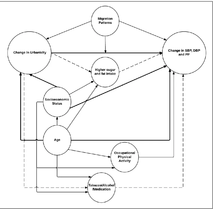
To examine the relationship between change in UI and BP, we estimated a series of mixed-effects longitudinal and cross-sectional models. For each outcome (SBP, DBP and PP), we modeled both initial levels and between survey change in UI, and moving as main exposures. We used a directed acyclic graph (DAG) to determine relevant confounders. Our minimally adjusted sets include age and SES variables (education level, log income per capita, and household wealth score) as confounders. Our DAG (fig. 1) shows that diet, occupational physical activity, WC, smoking status, alcohol intake, and
conditioning of sample characteristics to predict changes in BP and PP. Explanations for each simulation are based on the regression equation below:
𝑷𝒓𝒆𝒅𝒊𝒄𝒕𝒆𝒅 𝒗𝒂𝒍𝒖𝒆 = 𝛽0+ 𝛽1𝑋1+ 𝛽2𝑋2,𝑦𝑒𝑎𝑟+ 𝛽3𝑋3+ 𝛽4𝑋3𝑋1+ 𝛽5𝑋4+ 𝛽6𝑋4𝑋3+ 𝛽7𝑋5,𝑄𝑖𝑤𝑒𝑎𝑙𝑡ℎ+ 𝛽8𝑋6+ 𝛽9𝑋6𝑋1+ 𝛽10𝑋62+ 𝛽11𝑋62𝑋1+ 𝛽12𝑋63+ 𝛽13𝑋63𝑋1+Є
Where:
𝑋1= Change in UI
𝑋2= Survey Year (2005 and 2012 compared to 2002) 𝑋3= Previous UI
𝑋3𝑋1= Change in UI-Previous UI interaction 𝑋4= Moving (non-mover, movers)
𝑋4𝑋3= Moving-Previous UI interaction 𝑋5= Lagged wealth score quintile 𝑋6𝑛= Age to the n power
Є=Error term
𝛽0= Constant value when 𝑋𝑖= 0
𝛽1= Change in expected outcome per unit changes in UI 𝛽2= Change in expected outcome by survey year (2002,
2005, and 2012) 𝛽3= Change in expected outcome per unit
changes in previous UI
𝛽4= Change in expected outcome by change in UI-previous
UI interaction (increases in slope due to increments in
previous UI
𝛽5= Change in expected outcome by moving
𝛽6= Change in expected outcome by moving-previous UI
interaction (increases in previous UI slope due to moving)
𝛽7= Change in expected outcome by quintile of wealth
score compared to 1st quintile.
𝛽8= Change in expected outcome per unit changes in age 𝛽9= Change in expected outcome by age-change in UI
interaction (changes in age slope due to changes in UI)
𝛽10= Change in expected outcome per unit changes in
squared age
𝛽11= Change in expected outcome by squared age-change
in UI interaction (changes in squared age slope due to
changes in UI)
𝛽12= Change in expected outcome per unit changes in
cubic age
𝛽13= Change in expected outcome by cubic age-change in
UI interaction (changes in cubic age slope due to changes
FIGURE 1. Directed Acyclic Graph* of the Relationship between change in UI† and change in BP and PP‡
*Bolded and dashed lines represent the confounding and mediating pathways in the change in UI-change in BP relationship, respectively.
†Denotes changes in Urbanicity Index score between survey rounds.
Medication use was not included in the BP models because we considered medication use to be in the pathway between change in UI and change in BP/PP, implying that changes in UI may precede
medication use in our sample. Given how medication artificially lowers BP, adjusting for it in our models may attenuate the net effect of change in UI on our outcomes. Instead, to explore the role of
medication use in the UI-BP relationship, we estimated the association of change in UI and moving with the likelihood of using anti-hypertensive medication among participants with hypertension based on IDF cutoffs (SBP/DBP > 130/85). 9 Our final medication model include change in UI, squared change in UI, moving, age, survey year, and previous wealth quintiles. Models were estimated with mixed-effect longitudinal logistic regressions.
Finally, to determine the potential public health significance of the effect sizes observed in the analysis models, we assessed the relationship of SBP, DBP, and PP in 2005, separately, with the likelihood of hypertension-related mortality between 2005 and 2012 (N= 36 deaths).
Statistical analyses were conducted using STATA version 13.0 (Stata Corporation, College Station, TX, 2006). Detailed final model specifications and results are described in tables 2, 3, and 4. We consistently used α<0.05 and α<0.10 as the criterion for statistical significance for main effects and interaction terms, respectively.
Results
We describe sample characteristics among eligible participants from our longitudinal cohort in 1998 as well as characteristics by survey round (1998, 2002, 2005, and 2012) in table 1 and
supplemental table 2-5, respectively. In 1998, on average, participants were >40 y, lived in barangays
of moving, mothers tended to experience increases in UI compared to no changes or decreases throughout the follow-up period (Supp. Table 3) However, in 2005 more participants experienced UI decreases compared to no changes or UI increases. In non-movers, the highest mean SBP, DBP, and PP observed was >135, >79, and >55 mmHg in 2012, respectively (Supp. Table 4). In movers, the highest BP and PP values were found in 2005 (Supp. Table 5).
TABLE 1. Demographic characteristics of a longitudinal cohort of eligible participants in the Philippines in 1998*
N† 1938
Age‡ 41.92 ± 0.14
Urbanicity Index§ 38.95 ± 0.31
Systolic Blood Pressure# 113.45 ± 0.41
Diastolic Blood Pressure** 76.82 ± 0.27
Pulse Pressure†† 36.63 ± 0.23
Waist Circumference‡‡ 76.04 ± 0.21
Body Mass Index§§ 23.65 ± 0.09
Energy Intake## 1268.58 ± 12.92
Log Income per Capita*** 0.96 ± 0.01
Education Level†††
<6th Grade 1094(56.45)
7th-12th Grade 560(28.9)
>High School Education 284(14.65)
Migration Status‡‡‡
Non-Movers 1770(91.33)
Movers 168(8.67)
Direction of Urbanization§§§
No change 132(6.81)
Positive 1399(72.19)
Negative 288(14.86)
Missing 119(6.14)
*All data derived from the Cebu Longitudinal Health and Nutrition Survey (CLHNS) 1998, 2002, and 2005, and 2012 survey rounds. Our analytic sample includes 2107 participants aged 29-62 y in 1998 with complete blood pressure and select demographic data. Continuous and categorical variables are expressed as “mean ± S.E” and “count (percent)”, respectively.
†Total number of participants interviewed in 1998. ‡Based on self-reported age as of last birthday.
§ Multicomponent index that represents a gradient from rural to urban. It is derived from community surveys each survey year that reflects population size and density, community infrastructure, economic and environmental characteristics. Increasing continuous amount represent higher urban characteristics.
# Blood pressure (BP) was measured from 1998 in triplicate after a 10-minute seated rest using mercury sphygmomanometers. ** See #
††Calculated from the difference between Systolic and Diastolic Blood pressures. ‡‡ Measured by trained specialists.
§§ Height (m) and weight (kg) were measured at home by trained specialists using standardized methods.
## Estimated energy intake (kcals) in one 24-hr recall per survey round. We use conversion factors to account for moisture and fat retention due to cooking methods (e.g. boiling, braising, and frying).
*** Estimated weekly household income. Log transformation was performed due to income disparities in the Philippines.
††† Based on participant’s self-reported highest attained education level. Participants who did not know or reported “N/A” were considered to not have completed a single grade.
Changes and Secular trends in BP, PP, and UI
Overall, we observe increases in population mean SBP and DBP from 1998 through 2005 (figure 2). However, SBP and DBP diverge through the rest of follow-up, resulting in increases in PP between
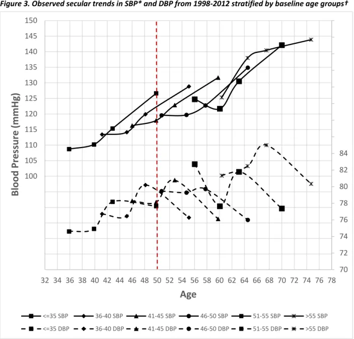
2005 and 2012. Mean and changes in BP and PP differ according to baseline age. Figure 3 shows BP trajectories, stratified by baseline age groups. A secular trend in SBP is apparent: Women who were 50 years old in 2012 had higher SBP and PP than women who were 50 years old in 1998 (fig. 3) indicating a secular trend of ~7 and ~9 mmHg, respectively. A similar secular trend was not observed for DBP. Women >55 y in 1998 had the highest mean SBP and DBP in 2012 (143.87 and 80.33 mmHg,
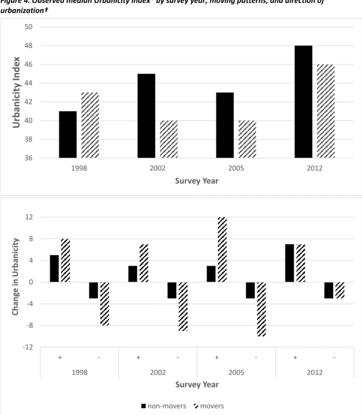
respectively). However, these and the second oldest age group had similarly high mean 2012 PP (>60 mmHg). We observe similar secular trends in BP and PP when only participants who were present through all survey rounds are considered (Supp. Figure 1). The number of barangays increased since the CLHNS began in 1983, as women moved throughout Metro Cebu. Mean UI for the original 33 barangays rose over time. Non-movers lived in more urban barangays from 2002 onward (figure 4). Participants who moved before 2002 and 2005 had the lowest median UI in the population. Evidently, changes in UI over time occurred in multiple directions in spite of moving: without change, from less to more urban, and vice-versa. Our figure 5 shows that movers tend to have higher UI increases than non-movers for most of follow-up. The largest contrast was observed in 2005, when movers had a median UI increase of 12 units compared to 3 in non-movers. Movers also had larger UI decreases compared to non-movers throughout follow-up. In spite of the direction of changes in UI, the same magnitude of change in UI from 2005 through 2012 was observed in both moving groups.
Change in BP models
covariates in our models. Interaction terms test heterogeneity of effects of change in UI on change in BP and PP across levels of previous UI; moving on changes in BP and PP across levels of previous UI, and change in UI on change in PP across age.
70 73 76 79 82 85 110
115 120 125 130 135
1994
1998
2002
2006
2010
2014
B
lood
Pr
es
su
re(
mmHg
)
Year
Mean SBP Mean DBP
Figure 2. Mean systolic and diastolic blood pressure* of CLHNS women by survey year
†
*Blood pressure (BP) was measured from 1998 in triplicate after a 10-minute seated rest using mercury sphygmomanometers. Means were derived from the average of three BP measurements. Solid lines represent SBP and dashed lines DBP. SBP and DBP values are shown on the left and right axis, respectively.
*Blood pressure (BP) was measured from 1998 in triplicate after a 10-minute seated rest using mercury sphygmomanometers. Means were derived from the average of three BP measurements. Solid lines represent SBP and dashed lines DBP. SBP and DBP values are shown on the left and right axis, respectively.
† Based on age when participants first participated from 1998-2012. Every data point represents blood pressure at
the mean age within each age group.
Figure 3. Observed secular trends in SBP* and DBP from 1998-2012 stratified by baseline age groups†
70 72 74 76 78 80 82 84
100 105 110 115 120 125 130 135 140 145 150
32 34 36 38 40 42 44 46 48 50 52 54 56 58 60 62 64 66 68 70 72 74 76 78
B
lood
Pr
es
su
re
(mmHg
)
Age
<=35 SBP 36-40 SBP 41-45 SBP 46-50 SBP 51-55 SBP >55 SBP
36 38 40 42 44 46 48 50
1998 2002 2005 2012
U
rba
ni
cit
y
Inde
x
Survey Year
Figure 4. Observed median Urbanicity Index* by survey year, moving patterns, and direction of urbanization†
-12 -8 -4 0 4 8 12
+ - + - + - +
-1998 2002 2005 2012
Ch
an
ge
in
Urb
an
ici
ty
Survey Year
non-movers movers
*Multicomponent index that represents a gradient from rural to urban. It is derived from community surveys each survey year that reflects population size and density, community infrastructure, economic and environmental characteristics. Increasing continuous amount represent higher urban characteristics.
SBP: The main effect of change in UI was positively and significantly associated with a 0.32
mmHg change in SBP (95%CI: 0.06, 0.57 P=0.015). The effects of change in UI and moving on change in SBP were significantly heterogeneous across levels of previous UI (95%CI: -0.02, -0.032E-1 and -0.19, 0.01 P<0.1). Survey year was significantly and positively associated with SBP increases >4 mmHg in 2005 and 2012 compared to 2002 (Table 2).
To aid in the understanding of SBP model results, we simulate specific conditions to predict the mean change in SBP through follow-up based on the estimated regression model below and offer and interpretation of results through a series of graphs. For example: (1) Movers who experienced no change
in UI and initially lived in barangays of UI levels of 30 have a predicted change in SBP of ~6.84 mmHg
(figure 5). (2) 35 y old movers who experienced no change in UI and lived in barangays of UI levels of 41
have a predicted change in SBP of ~4.71 mmHg (figure 6). Conditions are denoted below:
𝑷𝒓𝒆𝒅𝒊𝒄𝒕𝒆𝒅 𝑺𝑩𝑷 = 𝛽0+ 𝛽1𝑋1+ 𝛽2𝑋2,𝑦𝑒𝑎𝑟+ 𝛽3𝑋3+ 𝛽4𝑋3𝑋1+ 𝛽5𝑋4+ 𝛽6𝑋4𝑋3+ 𝛽7𝑋5,𝑄𝑖𝑤𝑒𝑎𝑙𝑡ℎ+ 𝛽8𝑋6+ 𝛽9𝑋6
2+ 𝛽
10𝑋63+Є
Where:
𝑋1= Change in UI (0, 5, 7) 𝑋2= Survey Year (on average) 𝑋3= Previous UI (30, 35, 40, 45, 50) 𝑋3𝑋1= Change in UI-Previous UI interaction 𝑋4= Moving (movers compared to non-movers) 𝑋4𝑋3= Moving-Previous UI interaction
𝑋5= Previous wealth score quintile (held constant) 𝑋6𝑛= Age to the n power (50 y)
Є =Error term
𝛽0= Constant value when 𝑋𝑖= 0
𝛽1= Change in expected SBP by unit changes in UI 𝛽2= Change in expected SBP by survey year
𝛽3= Change in expected SBP by unit changes in previous
UI
𝛽4= Change in expected SBP by change in UI-previous UI
interaction (increases in slope due to increments in
previous UI
𝛽5= Change in expected SBP by moving
𝛽6= Change in expected SBP by moving-previous UI
interaction (increases in previous UI slope due to moving)
𝛽7= Change in expected SBP by quintile of wealth score
compared to 1st quintile.
𝛽8= Change in expected SBP per unit changes in age 𝛽9= Change in expected SBP per unit changes in squared
age
𝛽10= Change in expected SBP per unit changes in age
Figure 5. Predicted change in SBP* by change in UI across previous UI†
Figure 6. Predicted change in SBP* by change in UI and age† 0
1 2 3 4 5 6 7 8
Non-movers Movers Non-movers Movers Non-movers Movers
0 5 7
Ch
an
ge
in
SB
P(m
m
H
g)
Change in UI
30 35 40 45 50
0 1 2 3 4 5 6 7
Non-movers Movers Non-movers Movers Non-movers Movers
0 5 7
Ch
an
ge
in
SB
P(m
m
H
g)
Change in UI
35 45 55 65
AGE
*Blood pressure (BP) was measured from 1998 in triplicate after a 10-minute seated rest using mercury sphygmomanometers. Means were derived from the average of three BP measurements. Solid lines represent SBP and dashed lines DBP. SBP and DBP values are shown on the left and right axis, respectively.
†Multicomponent index that represents a gradient from rural to urban. It is derived from community surveys each survey year that reflects population size and density, community infrastructure, economic and environmental characteristics. Increasing continuous amount represent higher urban characteristics.
PREVIOUS UI
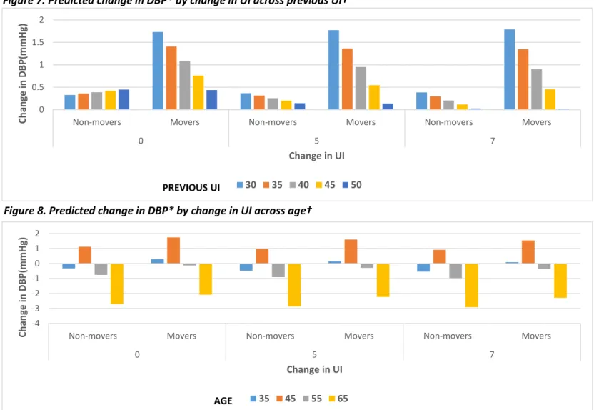
DBP: The effect of change in UI on change in DBP was heterogeneous according to previous
levels of UI (p<0.1). The main effect of moving and its interaction with previous UI were significantly associated with change in DBP, but in opposite directions (Table 2). Cubic age had a significantly positive relationship with change in DBP (0.54E-3|95%CI: 8.25E-5, 0.10E-3 P<0.05). Survey year was significantly associated with a >3 mmHg increase in 2005 and a decrease of just over 1 mmHg DBP in 2012,
compared to 2002.
To aid in the understanding of DBP model results, we simulate specific conditions to predict the average change in DBP through follow-up based on the estimated regression model below and offer and interpretation of results through a series of graphs. For example, (1)Movers who experienced no change
in UI and lived at a UI level of 30 have an expected change in DBP of ~1.73 mmHg (figure 7). (2) 35 y old
movers who experienced no change in UI and lived in barangays of UI levels of 41 have an expected
decrease in DBP of ~0.32 mmHg (figure 8). Conditions are denoted below:
𝑷𝒓𝒆𝒅𝒊𝒄𝒕𝒆𝒅 𝑫𝑩𝑷 = 𝛽0+ 𝛽1𝑋1+ 𝛽2𝑋2,𝑦𝑒𝑎𝑟+ 𝛽3𝑋3+ 𝛽4𝑋3𝑋1+ 𝛽5𝑋4+ 𝛽6𝑋4𝑋3+ 𝛽7𝑋5,𝑄𝑖𝑤𝑒𝑎𝑙𝑡ℎ+ 𝛽8𝑋6+ 𝛽9𝑋6
2+ 𝛽
10𝑋63+ Є Where:
𝑋1=Change in UI (0, 5, 7) 𝑋2= Survey Year (on average) 𝑋3= Previous UI (30, 35, 40, 45, 50) 𝑋3𝑋1= Change in UI-Previous UI interaction 𝑋4= Moving (movers compared to non-movers) 𝑋4𝑋3= Moving-Previous UI interaction
𝑋5= Previous wealth score quintile (held constant) 𝑋6𝑛= Age to the n power (50 y)
Є =Error term
𝛽0= Constant value when 𝑋𝑖= 0
𝛽1= Change in expected DBP per unit changes in UI
𝛽3= Change in expected DBP per unit changes in previous
UI
𝛽4= Change in expected DBP by change in UI-previous UI
interaction (increases in slope due to increments in previous UI
𝛽5= Change in expected DBP by moving
𝛽6= Change in expected DBP by moving-previous UI
interaction (increases in previous UI slope due to moving)
𝛽7= Change in expected DBP by quintile of wealth score
compared to 1st quintile.
𝛽8= Change in expected DBP per unit changes in age 𝛽9= Change in expected DBP per unit changes in squared
age
𝛽10= Change in expected DBP per unit changes in age
Figure 7. Predicted change in DBP* by change in UI across previous UI†
Figure 8. Predicted change in DBP* by change in UI across age† 0
0.5 1 1.5 2
Non-movers Movers Non-movers Movers Non-movers Movers
0 5 7
Ch
an
ge
in
DB
P(m
m
H
g)
Change in UI
30 35 40 45 50
PREVIOUS UI
-4 -3 -2 -1 0 1 2
Non-movers Movers Non-movers Movers Non-movers Movers
0 5 7
Ch
an
ge
in
DB
P(m
m
H
g)
Change in UI
35 45 55 65
AGE
*Blood pressure (BP) was measured from 1998 in triplicate after a 10-minute seated rest using mercury sphygmomanometers. Means were derived from the average of three BP measurements. Solid lines represent SBP and dashed lines DBP. SBP and DBP values are shown on the left and right axis, respectively.
†Multicomponent index that represents a gradient from rural to urban. It is derived from community surveys each survey year that reflects population size and density, community infrastructure, economic and environmental characteristics. Increasing continuous amount represent higher urban characteristics.
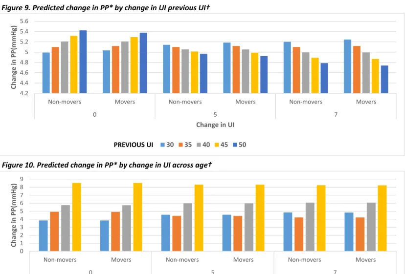
PP: The effect of change in UI on change in PP was significantly heterogeneous across levels of
previous UI and cubic age (p<.001). Neither the main effect of moving nor its interaction with previous UI are significantly associated with change in PP (Table 2). Survey year is positively associated with PP increases in both 2005 and 2012 compared to 2002. However, this association is significant only in 2012 (10.56 mmHg| 95%CI: 9.44, 11.67, p<0.01).
To aid in the understanding of PP model results, we simulate specific conditions to predict change in PP based on the estimated regression model below and offer interpretation of graphed results. For example, (1) Movers who experienced no change in UI and lived in barangays with UI levels
of 30 have an expected change in PP of ~5.03 mmHg (figure 9). (2) 35 y old movers who experienced no
change in UI and lived in barangays of UI levels of 41 have an expected increase in PP of ~3.84 mmHg
(figure 10). Conditions are denoted below.
𝑷𝒓𝒆𝒅𝒊𝒄𝒕𝒆𝒅 𝑷𝑷 = 𝛽0+ 𝛽1𝑋1+ 𝛽2𝑋2,𝑦𝑒𝑎𝑟+ 𝛽3𝑋3+ 𝛽4𝑋3𝑋1+ 𝛽5𝑋4+ 𝛽6𝑋4𝑋3+ 𝛽7𝑋5,𝑄𝑖𝑤𝑒𝑎𝑙𝑡ℎ+ 𝛽8𝑋6+ 𝛽9𝑋6𝑋1+ 𝛽10𝑋6
2+ 𝛽11𝑋62𝑋1+ 𝛽12𝑋63+ 𝛽13𝑋63𝑋1+ Є
Where:
𝑋1= Change in UI (0, 5, 7)
𝑋2= Survey Year (2005 and 2012 compared to 2002) 𝑋3= Lagged UI (30, 35, 40, 45, 50)
𝑋3𝑋1= Change in UI-Previous UI interaction 𝑋4= Moving (movers compared to non-movers) 𝑋4𝑋3= Moving-Previous UI interaction
𝑋5= Lagged wealth score quintile (held constant) 𝑋6𝑛= Age to the n power (50 y)
Є =Error term
𝛽0= Constant value when 𝑋𝑖= 0
𝛽1= Change in expected PP per unit changes in UI 𝛽2= Change in expected PP by survey year compared to
2002
𝛽3= Change in expected PP per unit changes in previous
UI
𝛽4= Change in expected PP by change in UI-previous UI
interaction (increases in slope due to increments in previous UI
𝛽5= Change in expected PP by moving
𝛽6= Change in expected PP by moving-previous UI
interaction (increases in previous UI slope due to moving) 𝛽7= Change in expected PP by quintile of wealth score
compared to 1st quintile.
𝛽8= Change in expected PP per unit changes in age 𝛽9= Change in expected PP by age-change in UI
interaction (changes in age slope due to changes in UI) 𝛽10= Change in expected PP per unit changes in squared
age
𝛽11= Change in expected PP by squared age-change in UI
interaction (changes in squared age slope due to changes in UI)
𝛽12= Change in expected PP per unit changes in cubic age 𝛽13= Change in expected PP by cubic age-change in UI
Figure 9. Predicted change in PP* by change in UI previous UI†
Figure 10. Predicted change in PP* by change in UI across age† 4.2
4.4 4.6 4.8 5 5.2 5.4 5.6
Non-movers Movers Non-movers Movers Non-movers Movers
0 5 7
Ch
an
ge
in
PP(m
m
H
g)
Change in UI
30 35 40 45 50
PREVIOUS UI
0 1 2 3 4 5 6 7 8 9
Non-movers Movers Non-movers Movers Non-movers Movers
0 5 7
Ch
an
ge
in
PP(m
m
H
g)
Change in UI
35 45 55 65
AGE
*Blood pressure (BP) was measured from 1998 in triplicate after a 10-minute seated rest using mercury sphygmomanometers. Means were derived from the average of three BP measurements. Solid lines represent SBP and dashed lines DBP. SBP and DBP values are shown on the left and right axis, respectively.
†Multicomponent index that represents a gradient from rural to urban. It is derived from community surveys each survey year that reflects population size and density, community infrastructure, economic and environmental characteristics. Increasing continuous amount represent higher urban
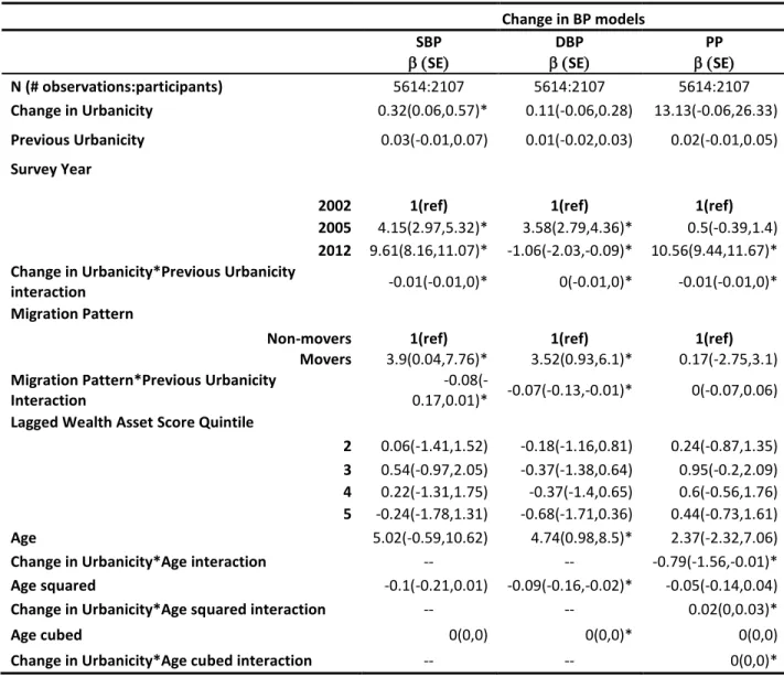
TABLE 2. Final Change in BP by change in UI model results output.
Change in BP models
SBP DBP PP
SE SE SE
N (# observations:participants) 5614:2107 5614:2107 5614:2107
Change in Urbanicity 0.32(0.06,0.57)* 0.11(-0.06,0.28) 13.13(-0.06,26.33)
Previous Urbanicity 0.03(-0.01,0.07) 0.01(-0.02,0.03) 0.02(-0.01,0.05)
Survey Year
2002 1(ref) 1(ref) 1(ref)
2005 4.15(2.97,5.32)* 3.58(2.79,4.36)* 0.5(-0.39,1.4)
2012 9.61(8.16,11.07)* -1.06(-2.03,-0.09)* 10.56(9.44,11.67)* Change in Urbanicity*Previous Urbanicity
interaction -0.01(-0.01,0)* 0(-0.01,0)* -0.01(-0.01,0)*
Migration Pattern
Non-movers 1(ref) 1(ref) 1(ref)
Movers 3.9(0.04,7.76)* 3.52(0.93,6.1)* 0.17(-2.75,3.1)
Migration Pattern*Previous Urbanicity Interaction
-0.08(-0.17,0.01)* -0.07(-0.13,-0.01)* 0(-0.07,0.06)
Lagged Wealth Asset Score Quintile
2 0.06(-1.41,1.52) -0.18(-1.16,0.81) 0.24(-0.87,1.35)
3 0.54(-0.97,2.05) -0.37(-1.38,0.64) 0.95(-0.2,2.09)
4 0.22(-1.31,1.75) -0.37(-1.4,0.65) 0.6(-0.56,1.76)
5 -0.24(-1.78,1.31) -0.68(-1.71,0.36) 0.44(-0.73,1.61)
Age 5.02(-0.59,10.62) 4.74(0.98,8.5)* 2.37(-2.32,7.06)
Change in Urbanicity*Age interaction -- -- -0.79(-1.56,-0.01)*
Age squared -0.1(-0.21,0.01) -0.09(-0.16,-0.02)* -0.05(-0.14,0.04)
Change in Urbanicity*Age squared interaction -- -- 0.02(0,0.03)*
Age cubed 0(0,0) 0(0,0)* 0(0,0)
Change in Urbanicity*Age cubed interaction -- -- 0(0,0)*
Change in BP by Change in UI
barangays. This shift is apparent in movers for PP. However, movers who previously lived in the least urban barangays were found to consistently have higher predicted BP compared to their more urban counterparts across levels of UI (figs 5, 7, and 9). In spite of moving and changes in UI, we predicted higher increases in SBP in 45 and 65 y olds compared to 35 and 55 y olds (fig 6). The highest increases and decreases in predicted DBP were also found in the former group (fig 8). Predicted PP was
consistently highest among older versus younger participants (fig 10). However, predicted change in PP for 35 y olds becomes higher than 45 y olds’ as UI increases.
Medication model
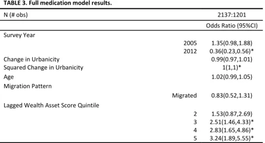
Compared to 2002, participants with hypertension in 2005 were 1.35 times (non-significantly) more likely to use medication (OR= 1.35| 95%CI: 0.98, 1.88) while participants in 2012 were ~64% less likely to use medication (OR= 0.36|95%CI: 0.23, 0.56 P<0.01). The association of medication use with change in urbanicity is positive, but non-linear, leveling off at higher change in urbanicity as indicated by the significant squared term. Moving was non-significantly associated with a 17% decreased likelihood of using medication. Being in the second wealth score quintile is non-significantly associated with a 53% increase likelihood of using medication compared to the lowest quintile. However, those in the third, fourth, and fifth are >2.5 times as likely to use anti-hypertensive medication (Table 3).
TABLE 3. Full medication model results.
N (# obs) 2137:1201
Odds Ratio (95%CI)
Survey Year
2005 1.35(0.98,1.88) 2012 0.36(0.23,0.56)*
Change in Urbanicity 0.99(0.97,1.01)
Squared Change in Urbanicity 1(1,1)*
Age 1.02(0.99,1.05)
Migration Pattern
Migrated 0.83(0.52,1.31) Lagged Wealth Asset Score Quintile
Mortality outcome models
SBP: Every 1 mm Hg increase in SBP in 2005 is significantly associated with a 4% increased
likelihood of hypertension-related mortality between 2005 and 2012 (95% CI: 1.02, 1.05 P<0.001). Every unit increase in age in 2005 is non-significantly associated with a 5% increased likelihood of
hypertension-related mortality between 2005 and 2012 (95%CI: 0.99, 1.11 P=0.094).
DBP: Every 1 mm Hg increase in DBP in 2005 is significantly associated with a 7% increased
likelihood of hypertension-related mortality between 2005 and 2012 (95%CI: 1.05, 1.09 P<0.001). Every unit increase in age in 2005 is significantly associated with a 7% increased likelihood of hypertension-related mortality in 2012 (95%CI: 1.01, 1.13 P=0.015).
PP: Every 1 mm Hg increase in PP in 2005 is significantly associated with a 4% increased
likelihood of hypertension-related mortality between 2005 and 2012 (95%CI: 1.02, 1.06 P<0.001). Every unit increase in age in 2005 is non-significantly associated with a 5% increased likelihood of
hypertension-related mortality between 2005 and 2012 (95%CI: 0.99, 1.11 P=0.076). Full mortality outcome model results output are displayed in table 4 below. TABLE 4. Mortality outcome model results *
Outcome Models
SBP DBP PP
95%CI 95%CI 95%CI
N (# obs) 2001 2001 2001
Mean SBP 1.04(1.02,1.05)† -- --
Mean DBP -- 1.07(1.05,1.09)† --
Mean PP -- -- 1.04(1.02,1.06)†
Age 1.05(0.99,1.11) 1.07(1.01,1.13)† 1.05(0.99,1.11)
*Models were adjusted for 2005 SBP, DBP, and PP, separately; and 2005 age. 36 total hypertension-related deaths were found in our final analytic sample.
CHAPTER 2: DISCUSSION AND SYNTHESIS
Discussion and Synthesis
Overview of major findings
From 1998 through 2012, we observed that SBP consistently increased and DBP peaked in 2005. As anticipated, we observed the greatest population-level increases in PP between 2005 and 2012. In 1998, the median SBP, DBP, and PP were 110, 78.67, and 40 mmHg, respectively. Their 2012 median values were 124.33, 75.67, and 49.33 mmHg, respectively. Trends in BP highlight important secular and age-related changes in blood and pulse pressures. We observed that younger participants had higher SBP, lower DBP, and higher PP in 2012 compared to individuals of the same age in 1998. Restriction of this analysis to those women with complete data suggest that this is a true secular trend, not explained by the higher mortality and thus lower representation of older women in the 2012 sample.
Modernization and urban development were responsible for UI increases in the original 33 CLHNS barangays. At an individual level, UI increases among movers reflected the tendency for these to move from less to more urban barangays. Individual decreases in UI do not necessarily indicate
Different communities may have the same UI score according to their individual components that drive urbanicity (i.e. population density, access to hospitals, etc.). Thus, participants may have moved between communities with different characteristics but the same UI score.
Our observed age-related BP changes align with the notion that SBP and DBP increase in early adulthood. The continued SBP increase and DBP decrease from middle adulthood through later in life associated with age-related arterial stiffness and peripheral vascular resistance18,19, respectively, thus led to higher PP with age.
Comparison with previous literature
middle-adulthood with higher DBP. Furthermore, mean rates of DBP increase are ~3 times faster in the youngest versus oldest cohort, even after adjusting for BMI. While many large cross-sectional
epidemiological studies document secular decreases in SBP and DBP over time, these fail to account for individual change in BP. 24-26 Recent work from the China Health and Nutrition Survey (CHNS) highlights secular and temporal changes in blood pressure through an 18-year period.27 The oldest CHNS women (born in 1940) experienced greater increases in SBP and DBP from 1991 through 2009 compared to their younger counterparts (born in 1970s) across levels of UI. However, the difference in DBP increases between these age cohorts was larger at lower UI.
The current literature investigating the urbanicity-BP relationship is mostly comprised of cross-sectional studies, with few exceptions from prospective longitudinal cohort studies.20-23, 27 Studies incorporating migration into the mix are less prevalent. Despite the inability to infer how temporal changes in urbanicity relate to BP and PP from cross-sectional studies, we can’t ignore important previous insights that help explain the complex nature of urban health. In previous work in the contexts of India and Cameroon28, 29, exposure to urbanicity has previously been quantified based on
and DBP were similarly comparable across cohorts residing in the 75th percentile of urbanicity. However, cohort differences in DBP in women were statistically significant only in the context of low urbanicity.
Limitations and Strengths
The present study has various limitations worth mentioning. Undoubtedly, our observed and estimated changes in BP may be affected by the level of medication awareness and actual medication use in participants. While interviewees were asked specifically about use of medications to treat hypertension, some participants may have misreported on their medication use with respect to its purpose. Similarly, participant mortality causes were reported by available household members and not medical records. However, a comparison of reported versus death certificate-listed cause of death in a subset of participants indicated a high level of concordance. Another weakness is that by design, our study population is contained within the Metro Cebu area. Therefore, it is currently impossible to assess how migration affects BP among participants who out-migrated to the capital (Manila) or other cities or countries, thus limiting the generalizability of our findings. Effectively, 78% of attrition in the CLHNS is attributed to out-migration from the Metro Cebu area.31 We also only considered participants who moved between survey years as migrants with no consideration of migration frequency within survey intervals, which ranges from 4 to 7 years We expect that frequent migrants may differ from less frequent counterparts with respect to exposure to UI through their lives.
crucial element of causal inference. Another strength is the use of our multi-component UI. The use of continuous UIs has been previously shown to better represent environmental heterogeneity within regions compared to dichotomous urbanicity variables (urban/rural)typically used in a variety of international settings.16, 32-37
Public Health Implications and Conclusions
Our findings have important public health implications given the independent associations of PP with stroke, myocardial infarction, and other CVD outcomes.6,19,21,38 This is further reinforced by the observed secular and temporal BP and PP changes in the youngest and oldest CLHNS participants. Our study echoes previous work in the CHNS highlighting the importance of BP screening in rural areas.27 Our work adds attention to the young and migrant CLHNS populations. Efficient blood pressure surveillance systems are vital for the proper monitoring of BP and PP trajectories in the adult population. Age-specific efforts may be required to raise awareness among Filipino individuals at different stages of adulthood about the importance of tracking blood pressure, maintenance of healthy blood pressure, and how proximal factors influenced by the environment (e.g. air and noise pollution, highly processed foods, crime, stress) affect it. BP monitoring and surveillance may help shed light on the prevalence and incidence of untreated hypertension across ages in rural areas with poor access to hospitals. This is crucial given that hypertension is considered as one of the most important modifiable risk factors for CVD events.
To understand how urban life affects BP, it is crucial to consider the magnitude of change in UI, when (in age) this change occurs, and the levels of UI from where these changes are occur over time (be it by staying or migrating). We found that migrants who previously lived in the most rural barangays have the highest predicted increases in SBP and DBP, and PP as their exposure to UI increases. In addition, we found that at the same level of previous UI, the oldest individuals have the highest
APPENDIX 1: ADDITIONAL RESULTS
Supplemental Table 1. Correlation matrix of household asset variables* included in household wealth score.
Owna tv
Own a fridge
Own a bicycle
Own a vehicle
Own a china
Number of rooms in house
Toilet Quality
Housing Quality
Source of Water
Access to electricity
Cooking Fuel
Own a tv 1
Own a fridge 0.42 1
Own a bicycle 0.19 0.2 1
Own a vehicle 0.19 0.3 0.11 1
Own a china 0.18 0.27 0.09 0.17 1
Number of rooms in
house 0.33 0.31 0.14 0.21 0.14 1
Toilet Quality 0.37 0.32 0.12 0.06 0.13 0.12 1
Housing Quality 0.39 0.47 0.19 0.3 0.26 0.37 0.3 1
Source of Water 0.25 0.21 0.1 0.08 0.12 0 0.4 0.2 1
Access to electricity -0.53 -0.3 -0.17 -0.1 -0.12 -0.24 -0.47 -0.36 -0.35 1
Cooking Fuel 0.29 0.15 0.11 0.04 0.06 0.01 0.37 0.17 0.3 -0.36 1
* The list of assets were based on the International Wealth Index (IWI). We modified the list of assets from the IWI based on available household-level characteristics assessed during the 1994 CLHNS household survey round by key informants and trained interviewers.
SUPPLEMENTAL TABLE 1.1. NOTATION KEY FOR SUPPLEMENTARY TABLES 2-5
* All data derived from the Cebu Longitudinal Health and Nutrition Survey (CLHNS) 1998, 2002, and 2005, and 2012 survey rounds. Our analytic sample includes 2107 participants aged 29-62 y in 1998 with complete blood pressure and select demographic data. Continuous and categorical variables are expressed as “mean ± S.E” and “count (percent)”, respectively.
† Total number of participants interviewed in each survey round. ‡ Based on self-reported age as of last birthday.
§ Multicomponent index that represents a gradient from rural to urban. It is derived from community surveys each survey year that reflects population size and density, community infrastructure, economic and environmental characteristics. Increasing continuous amount represent higher urban characteristics.
# Participant’s change in UI score since the previous survey. 1998 values denote changes in UI since the 1994 CLHNS survey round.
** Blood pressure (BP) was measured from 1998 in triplicate after a 10-minute seated rest using mercury sphygmomanometers.
†† See **
‡‡ Calculated from the difference between Systolic and Diastolic Blood pressures. §§ Measured by trained specialists.
## Height (m) and weight (kg) were measured at home by trained specialists using standardized methods.
*** Estimated energy intake (kcals) in one 24-hr recall per survey round. We use conversion factors to account for moisture and fat retention due to cooking methods (e.g. boiling, braising, and frying). ††† Estimated weekly household income. Log transformation was performed due to income
disparities in the Philippines.
‡‡‡ Based on participant’s self-reported highest attained education level. Participants who did not know or reported “N/A” were considered to not have completed a single grade.
SUPPLEMENTAL TABLE 2. Characteristics of a Longitudinal Cohort of Eligible Adult Filipino Women Participants from 1998-2012*
Survey Year 1998 2002 2005 2012
n† 1938 2072 2008 1818
Mean (S.E.) Median Mean (S.E.) Median Mean (S.E.) Median Mean (S.E.) Median
Age‡ 41.92(0.14) 41.22 45.87(0.13) 45.17 48.77(0.13) 48.03 55.56(0.14) 54.78
Urbanicity Index§ 38.95(0.31) 41 41.3(0.31) 45 40.49(0.3) 43 43.96(0.3) 47
Systolic Blood Pressure** 113.45(0.41) 110 114.48(0.42) 110.67 119.62(0.45) 119.33 129.66(0.57) 124.33
Diastolic Blood Pressure†† 76.82(0.27) 78.67 76.61(0.28) 75.33 79.63(0.28) 80 76.76(0.3) 75.67
Pulse Pressure‡‡ 36.63(0.23) 40 37.87(0.25) 37.33 39.99(0.28) 40 52.9(0.37) 49.33
Waist Circumference§§ 76.04(0.21) 75.2 78.59(0.22) 78 80.93(0.26) 80.6 82.05(0.27) 81.62
Body Mass Index## 23.65(0.09) 23.29 24.34(0.09) 24.19 24.35(0.1) 24.17 24.85(0.11) 24.71
Energy Intake*** 1268.58(12.92) 1170.63 1208.02(13.21) 1106.59 1226.73(13.7) 1112.24 1082.86(13.92) 961
Log Income per Capita††† 0.96(0.01) 0.89 0.96(0.01) 0.89 0.95(0.01) 0.89 1.36(0.01) 1.27
N % N % N % N %
Education Level ‡‡‡
<6th Grade 1,094 56.45 1,212 58.49 1,172 58.37 1,071 58.91
7th-12th Grade 560 28.9 587 28.33 574 28.59 514 28.27
>High School Education 284 14.65 273 13.18 262 13.05 233 12.82
Migration Status§§§
Stayed 1,770 91.33 1,943 93.77 1,930 96.12 1,107 60.89
Moved 168 8.67 129 6.23 78 3.88 702 38.61
missing -- -- -- 9 0.5
Direction of Urbanization###
No change 132 6.81 177 8.54 390 19.42 123 6.77
Positive 1,399 72.19 1,511 72.92 608 30.28 1,281 70.46
Negative 288 14.86 372 17.95 1,009 50.25 414 22.77
missing 119 6.14 12 0.58 1 0.05 --
SUPPLEMENTAL TABLE 3. Characteristics of a Longitudinal Cohort of Eligible Adult Filipino Women Participants by Moving Status 1998-2012*
Survey year 1998 2002 2005 2012
n† 1938 2072 2008 1818
Stayed Moved Stayed Moved Stayed Moved Stayed Moved
Age‡ 42.04
(0.14) 40.65 (0.42) 45.97 (0.14) 44.34 (0.5) 48.84 (0.14) 47.17 (0.63) 55.83 (0.18) 55.09 (0.22)
Urbanicity Index§ 38.82
(0.33) 40.29 (0.88) 41.35 (0.32) 40.49 (1.17) 40.55 (0.31) 38.97 (1.34) 45.29 (0.35) 41.93 (0.52)
Change in Urbanicity#
3.5 (0.09) 0.67 (1.02) 3.02 (0.1) 0.68 (1.22) -0.63 (0.1) -4.31 (1.59) 3.74 (0.13) 3.25 (0.31)
Systolic Blood Pressure** 113.37
(0.43) 114.33 (1.42) 114.45 (0.44) 114.93 (1.68) 119.6 (0.46) 120.28 (2.08) 129.76 (0.74) 129.41 (0.91) Diastolic Blood Pressure†† 76.8 (0.28) 77.02 (1) 76.59 (0.28) 76.95 (1.13) 79.59 (0.28) 80.57 (1.15) 76.76 (0.38) 76.77 (0.47)
Pulse Pressure‡‡ 36.57
(0.24) 37.31 (0.76) 37.87 (0.26) 37.98 (0.84) 40 (0.29) 39.71 (1.38) 53 (0.47) 52.64 (0.58)
Waist Circumference§§ 76.01
(0.22) 76.42 (0.7) 78.66 (0.22) 77.62 (0.79) 80.94 (0.27) 80.78 (1.08) 82.33 (0.34) 81.6 (0.45)
Body Mass Index## 23.6
(0.1) 24.15 (0.3) 24.37 (0.1) 23.89 (0.34) 24.34 (0.1) 24.69 (0.43) 24.99 (0.14) 24.63 (0.18)
Total Energy Intake*** 1262.89
(13.5) 1328.52 (44.36) 1206.11 (13.6) 1236.81 (56.01) 1227.92 (14.03) 1197.08 (62.22) 1106.95 (18.65) 1045.52 (20.68)
Income per Capita††† 0.96
(0.01) 1.02 (0.03) 0.96 (0.01) 1.05 (0.06) 0.95 (0.01) 0.94 (0.04) 1.37 (0.02) 1.35 (0.02) Urbanization Direction‡‡‡
no change 126 (7.12) 6 (3.57) 173 (8.9) 4 (3.1) 387 (20.05) 3 (3.85) 77
(6.96) 46 (6.55) less to more urban 1333
(75.31) 66 (39.29) 1444 (74.32) 67 (51.94) 584 (30.26) 24 (30.77) 806 (72.81) 468 (66.67) more to less urban 228
(12.88) 60 (35.71) 317 (16.31) 55 (42.64) 958 (49.64) 51 (65.38) 224 (20.23) 188 (26.78) missing 83 (4.69) 36 (21.43) 9 (0.46) 3 (2.33) 1
(0.05) -- -- --
SUPPLEMENTAL TABLE 4. Longitudinal Characteristics of Non-Movers by Direction of Urbanization from 1998-2012*
Survey Year 1998 2002 2005 2012
n† 1938 2072 2008 1818
0 + - 0 + - 0 + - 0 + -
Age‡ 42.99
(0.58) 42.01 (0.16) 42.7 (0.43) 45.05 (0.45) 46.12 (0.16) 45.95 (0.35) 48.61 (0.3) 49.01 (0.27) 48.83 (0.19) 55.81 (0.7) 55.89 (0.21) 55.61 (0.39)
Urbanicity Index§ 35.08
(1.45) 41.69 (0.33) 24.13 (0.81) 35.58 (1.33) 43.62 (0.34) 34.61 (0.77) 46.67 (0.72) 39.32 (0.52) 38.83 (0.44) 47.27 (1.45) 44.43 (0.42) 47.7 (0.59) Change in
Urbanicity# 0(0)
5.01 (0.07)
-3.34
(0.13) 0 (0)
4.88 (0.08)
-3.83
(0.16) 0(0)
3.91 (0.11)
-3.65
(0.1) 0 (0)
5.9 (0.1) -2.75 (0.11) Systolic Blood Pressure** 115.79 (1.69) 113.03 (0.48) 115.05 (1.36) 113.6 (1.52) 114.69 (0.51) 114.09 (1.11) 120.38 (1.04) 119.44 (0.83) 119.38 (0.64) 135.56 (2.93) 129.7 (0.87) 127.98 (1.59) Diastolic Blood Pressure†† 77.58 (1.05) 76.63 (0.32) 77.47 (0.8) 75.76 (0.93) 76.91 (0.33) 75.67 (0.69) 79.5 (0.64) 79.35 (0.51) 79.77 (0.41) 78.94 (1.5) 76.8 (0.45) 75.84 (0.81)
Pulse Pressure‡‡ 38.21
(1.02) 36.4 (0.27) 37.58 (0.81) 37.84 (0.92) 37.77 (0.3) 38.42 (0.64) 40.88 (0.7) 40.09 (0.54) 39.61 (0.38) 56.62 (1.94) 52.9 (0.55) 52.14 (1.06) Waist Circumference§§ 74.43 (0.8) 76.36 (0.26) 74.83 (0.63) 77.82 (0.81) 78.83 (0.26) 78.45 (0.54) 81.02 (0.61) 80.62 (0.52) 81.11 (0.37) 81.57 (1.27) 82.28 (0.39) 82.78 (0.8)
Body Mass Index## 22.88
(0.35) 23.8 (0.11) 22.92 (0.29) 23.98 (0.37) 24.4 (0.11) 24.55 (0.23) 24.3 (0.24) 24.24 (0.18) 24.41 (0.14) 24.91 (0.53) 24.93 (0.16) 25.23 (0.33) Total Energy Intake*** 1218.74 (55.83) 1289.57 (15.67) 1171.54 (32.47) 1125.37 (42.9) 1215.31 (15.93) 1211.98 (33.2) 1190.99 (31.29) 1240.97 (25.24) 1235.56 (20.05) 1090.52 (73.48) 1071.1 (20) 1241.57 (50.94)
Income per Capita††† 1.02
SUPPLEMENTAL TABLE 5. Longitudinal Characteristics of Movers by Direction of Urbanization from 1998-2012*
Survey Year 1998 2002 2005 2012
n† 1938 2072 2008 1818
0 + - 0 + - 0 + - 0 + -
Age‡ 38.56
(1.53) 41.35 (0.66) 41.59 (0.71) 38.48 (2.07) 44.3 (0.64) 44.95 (0.82) 44.7 (4.19) 48.07 (1.21) 46.89 (0.74) 57.91 (1.14) 55.22 (0.27) 54.07 (0.39)
Urbanicity Index§ 44.67
(1.91) 44.62 (1.26) 35.52 (1.25) 40 (10.34) 44.52 (1.62) 34.78 (1.46) 50.33 (0.33) 44.75 (2.26) 35.59 (1.55) 41.39 (1.93) 41.69 (0.69) 42.66 (0.81)
Change in Urbanicity# 0 (0)
9.89 (0.89)
-9.42
(0.91) 0 (0)
10.49 (1.11)
-11.22
(1.11) 0 (0)
12.29 (1.97)
-12.37
(1.1) 0 (0)
7.31 (0.24) -6.07 (0.49) Systolic Blood Pressure** 105 (4.28) 115.41 (2.39) 116.22 (2.18) 115.17 (4.68) 114.29 (2.26) 116.19 (2.81) 140.22 (36.3) 120.12 (4.22) 119.18 (1.66) 133.53 (4.06) 129.57 (1.13) 128.03 (1.66) Diastolic Blood Pressure†† 74 (3.27) 76.33 (1.54) 79.58 (1.61) 78.83 (3.76) 76.36 (1.61) 77.67 (1.76) 83.56 (18.19) 81 (2.25) 80.19 (1.1) 79.7 (2.16) 76.76 (0.57) 76.1 (0.91)
Pulse Pressure‡‡ 31
(1.91) 39.08 (1.31) 36.64 (1.13) 36.33 (1.99) 37.94 (1.09) 38.52 (1.44) 56.67 (19.16) 39.12 (2.66) 38.99 (1.32) 53.82 (2.55) 52.81 (0.75) 51.92 (0.96) Waist Circumference§§ 74.03 (2.46) 76.63 (1.15) 78.37 (1.13) 82.43 (5.84) 76.97 (1.05) 77.96 (1.27) 83.13 (2.43) 78.91 (1.78) 81.51 (1.42) 79.77 (1.89) 81.09 (0.55) 83.32 (0.86)
Body Mass Index## 23.68
(1.17) 24.28 (0.48) 24.99 (0.5) 25.82 (2.79) 23.49 (0.48) 24.21 (0.5) 26.25 (0.81) 23.92 (0.82) 24.95 (0.54) 24.27 (0.77) 24.37 (0.22) 25.37 (0.35) Total Energy Intake*** 1339.41 (104.82) 1234.36 (55.51) 1388.14 (78.74) 1177.38 (75.69) 1176.05 (61.7) 1282.13 (105.61) 1052.71 (328.35) 1134.66 (77.88) 1234.95 (86.38) 924.23 (83.76) 994.46 (24.26) 1202.3 (41.61)
Income per Capita††† 0.9
70 75 80 85
100 105 110 115 120 125 130 135 140 145 150
30 35 40 45 50 55 60 65 70 75 80
Bl
ood
Pr
ess
ur
e(
mm
Hg
)
Age
<=35
36-40
41-45
46-50
51-55
>55
<=35
36-40
41-45
46--50
51-55
>55
Supplemental Figure 1. Observed secular trends in SBP* and DBP from 1998-2012 stratified by
baseline age groups† among participants with full participation
*Blood pressure (BP) was measured from 1998 in triplicate after a 10-minute seated rest using mercury sphygmomanometers. Means were derived from the average of three BP measurements. Solid lines represent SBP and dashed lines DBP. SBP and DBP values are shown on the left and right axis, respectively.
REFERENCES
1. Popkin, B. M., Adair, L. S., & Ng, S. W. (2012). NOW AND THEN: The Global Nutrition Transition: The Pandemic of Obesity in Developing Countries. Nutrition Reviews, 70(1), 3–21.
2. Adair LS. Dramatic rise in overweight and obesity in adult Filipino women and risk of hypertension. Obes Res. Vol 12, (1335-1341), 2004.
3. Food and Nutrition Research Institute of the Philippines. Emerging Nutrition Concerns:
Prevalence of Non-Communicable Disease Risk factors: Time Trends from 1998 to 2015 National Nutrition Survey and Updating of the Nutritional Status of Filipino Children and Other
Population Groups. FNRI of the Philippines. 2016 Calabarzon Regional Dissemination Forum; July 28, 2016.
4. Krakoff LR, Gillespie RL, Ferdinand KC, et al. 2014 Hypertension Recommendations From the Eighth Joint National Committee Panel Members Raise Concerns for Elderly Black and Female Populations. J Am Coll Cardiol.2014;64(4):394-402.
5. Okada K, Iso H, Cui R, Inoue M. Pulse pressure is an independent risk factor for stroke among middle-aged Japanese with normal systolic blood pressure : the JPHC study. Journal of
Hypertension; 29(2):319-324; 2011.
6. Rourke MO, Frohlich ED. Pulse Pressure: Is this a Clinically Useful Risk Factor? Journal of
Hypertension. 2010:372-374.
7. Domanski M, Mitchell G, Neaton JD, Norman J, Svendsen K. Pulse Pressure and Cardiovascular Disease – Related Mortality. JAMA. 2002; 287(20):2677-2683.
8. Thomas F, Blacher J, Benetos A, Safar ME, and Pannier B. Cardiovascular risk as defined in the 2003 European blood pressure classification : the assessment of an additional predictive value of pulse pressure on mortality. Journal of Hypertension. 2008, (26): 1072-1077.
9. The International Diabetes Federation. The IDF consensus worldwide definition of the metabolic syndrome. http://www.idf.org/metabolic-syndrome. Last accessed on 10/22/2016.
11. Pereira MA, FitzerGerald SJ, Gregg EW, Joswiak ML, Ryan WJ, Suminski RR, Utter AC, Zmuda JM. A collection of Physical Activity Questionnaires for health-related research. Med Sci Sports Exerc. 1997;29:S1-205.
12. Patel A, Huang KC, Janus ED, Gill T, Neal B, Suriyawongpaisal P, Wong E, Woodward M, Stolk RP. Is a single definition of the metabolic syndrome appropriate?--A comparative study of the USA and Asia. Atherosclerosis. 2006;184:225-232.
13. Forrest KY, Bunker CH, Kriska AM, Ukoli FA, Huston SL, Markovic N. Physical activity and
cardiovascular risk factors in a developing population. Med Sci Sports Exerc. 2001;33:1598-1604.
14. FNRI. Food Composition Tables Recommended for Use in the Philippines. Manila, Philippines:
Food and Nutrition Research Institute.; 1997.
15. Smits, J. & Steendijk, R. The International Wealth Index (IWI). Social Indicators Research (2015) 122: 65.
16. Dahly DL, Adair LS. Quantifying the urban environment: a scale measure of urbanicity outperforms the urban-rural dichotomy. Soc Sci Med. 2007;64:1407-1419.
17. Office of Population Studies, University of San Carlos; Carolina Population Center, The University of North Carolina at Chapel Hill Nutrition Center of the Philippines. The Cebu Longitudinal Health and Nutrition Survey, Survey Procedures.
18. Tin LL, Beevers DG, and Lip GYH. Systolic vs diastolic blood pressure and the burden of hypertension. Journal of Human Hypertension (2002) 16, 147-150.
19. Franklin SS, Larson MG, Khan SA, Wong ND, Leip EP, Kannel WB, and Levy D (2001). Does the Relation of Blood Pressure to Coronary Heart Disease Risk Change With Aging? Circulation; 103:1245-1249.
20. Cheng, S., Xanthakis, V., Sullivan, L. M., & Vasan, R. S. (2012). Blood Pressure Tracking Over the Adult Life Course: Patterns and Correlates in the Framingham Heart Study. Hypertension, 60(6), 1393–1399.