P
OWERINGD
EMAND: S
OLARP
HOTOVOLTAICS
UBSIDIES INC
ALIFORNIAKenneth D. Reddix II
A dissertation submitted to the faculty of the University of North Carolina at Chapel Hill in par-tial fulfillment of the requirements for the degree of Doctor of Philosophy in the Department of
Economics.
Chapel Hill 2015
c
2015
ABSTRACT
KENNETH D. REDDIX II: Powering Demand: Solar Photovoltaic Subsidies in California. (Under the direction of Brian McManus)
I dedicate this dissertation to my best friend, soulmate, and wife Cynthia. I would not be here today without your guidance, patience, unending support, and unconditional love.
You are truly amazing. Te amo Bella.
To my father Ken and my mother Susan, I want to express my deep appreciation for your dedication to my education, and the unconditional love and support you have given me
ACKNOWLEDGMENTS
TABLE OF CONTENTS
LIST OF TABLES . . . viii
LIST OF FIGURES . . . x
1 Introduction . . . 1
2 Institutional Background . . . 6
2.1 Solar Panels . . . 6
2.2 Subsidies and Tax Credits . . . 8
3 Model . . . 16
3.1 Households’ Problem . . . 16
3.2 Utility From Purchase . . . 18
3.3 Utility From Waiting . . . 22
3.4 Tax Policies . . . 23
3.5 Identification . . . 28
4 Data . . . 29
5 Estimation . . . 44
6 Results . . . 53
6.1 Static Models . . . 53
6.2 Dynamic Models . . . 56
6.3 Model Fit . . . 61
6.4 Elasticities . . . 63
8 Conclusion . . . 78
A Assumptions and Copulas . . . 79
A.1 Assumptions . . . 79
A.2 Brief Summary of Copula Functions . . . 80
B Additional Data Considerations . . . 83
C Additional Results and Counterfactual Simulations . . . 97
C.1 Additional Count Regression Results . . . 97
C.2 Estimation Results . . . 97
C.3 Counterfactual Simulations . . . 100
LIST OF TABLES
4.1 Household Characteristics (Purchasers) . . . 32
4.2 Household Characteristics (Full Population) . . . 34
4.3 Household Characteristics (Reduced Population from Survey) . . . 36
4.4 Full Set of Solar Panels . . . 43
4.5 Set of Purchased Solar Panels . . . 43
6.1 Number of Installations Per Day (Unconditional) . . . 54
6.2 Number of Installations Per Day Conditional on 6-Month Bins . . . 54
6.3 Models for Daily Installations . . . 55
6.4 Static Model Estimation Results . . . 57
6.5 First Stage Estimation Results from 2001-2010 . . . 58
6.6 Second Stage Estimation Results . . . 60
6.7 Empirical vs Simulated Choice Probabilities . . . 64
6.8 Empirical vs Simulated Choice Probabilities by Capacity Bin . . . 65
6.9 Price Elasticity Given a 1% Increase in Price . . . 66
6.10 Marginal Effect of a 1% Increase in Efficiency Rates . . . 67
7.1 Change in Purchase without Government Intervention (Pes) . . . 69
7.2 Change in Purchase (%) without Government Intervention by Capacity (Pes) . . . . 70
7.3 Additional Capacity (kW) Installed with Government Intervention (Pes) . . . 72
7.4 Marginal Increase in Installations given a 10% Increase in the Subsidy (Pes) . . . . 76
7.5 Marginal Increase in Installations given a 10% Increase in the Subsidy (AR) . . . . 76
7.6 Number of Installations under Pessimism without Uncertainty . . . 77
C.1 Models for Semi-Annual Installations . . . 97
C.2 Second Stage Estimation Results (Reduced Sample) . . . 98
C.3 Second Stage Estimation Results with an Additional Regime Change . . . 99
C.4 Change in Purchase without Government Intervention (PF) . . . 101
C.5 Change in Purchase (%) without Government Intervention by Cap (PF) . . . 102
C.6 Additional Capacity (kW) Installed with Government Intervention (PF) . . . 103
C.7 Change in Purchase without Government Intervention (AR) . . . 104
C.8 Change in Purchase (%) without Government Intervention by Cap (AR) . . . 105
LIST OF FIGURES
2.1 Subsidy Rates over Time . . . 9
2.2 Subsidy Rate and Number of Installations Per Period . . . 11
2.3 Average Tax Credit Per Watt . . . 12
2.4 Medium Capacity Solar Panel System Prices in San Francisco . . . 15
3.1 Case 1: Perfect Foresight . . . 24
3.2 Case 2: Pessimistic Beliefs . . . 26
3.3 Case 3: Auto-Renewal Beliefs . . . 27
4.1 Electricity Prices by Utility Company . . . 37
4.2 Price Per Watt by MSA . . . 39
4.3 Price Per Watt by Capacity Bin in Los Angeles . . . 40
4.4 Efficiency Rates over Time . . . 42
7.1 Additional Capacity Installed with Subsidy by Capacity Bin . . . 73
7.2 Number of Installations as a Function of % of Subsidy . . . 75
CHAPTER 1 INTRODUCTION
In 2013, the market for solar panel systems reached a value of $12 billion dollars with an average annual growth rate of 50%. High growth rates in the solar market are attributed to the widespread use of subsidies and tax credits by federal and state governments, and sharp reduc-tions in the cost of solar panels. The U.S. Energy Information Administration reports that federal funding for solar power increased 530%, from $179 million to $1.13 billion dollars, between the years of 2007 to 2010.1 Since 2001, California has provided over $2 billion dollars in demand-side subsidies for solar panel systems, and consequently leads the United States in redemand-sidential solar electricity generation.
For a household participating in a durable good market, the decisions of when to purchase and what to purchase are both important. Particularly in markets that are characterized by rapid technological innovation and declining market prices, a household might delay the decision to purchase for the option value of waiting. The California residential market for solar panel systems is similarly characterized by steady technological innovation and falling market prices, but is also subjected to multiple short-lived subsidy regimes. Short-lived subsidy regimes, lasting 2 to 3 years, are used to temporarily reduce prices and stimulate households’ demand for solar panel systems. For these reasons, it is important to model the demand for solar panel systems in a dynamic framework. I introduce a structural model of dynamic demand for solar panel systems that includes uncertainty about future prices and future subsidies, and I estimate the model using a newly assembled data set at the household level. The model is used to investigate the implications of multiple short-lived subsidy regimes, evaluate price elasticities, and measure the effectiveness
of demand-side subsidies.
In a dynamic setting, households make decisions considering both the expectation regarding the change in prices over time and the level of prices within a period. In the solar panel market, forming expectations about the change in prices requires households to consider the change in market prices for solar panel systems and the existence of future subsidy regimes. Market prices for solar panel systems decline throughout the sample period with the price of an average solar panel system falling more than 20%. To account for market price uncertainty, households are not fully informed about the pricing process for solar panel systems, but instead expect future market prices to follow a Markovian process. This assumption, while simple, allows for households to be correct on average about the evolution of prices while still accounting for price uncertainty. Households are fully informed about the schedule of subsidy rates within a particular regime, but lack information about future regimes. To account for this uncertainty, households are assumed to have beliefs regarding the existence of future regimes. Three separate deterministic belief structures are tested in the paper. The estimation results show that demand is fairly robust to assumptions regarding households beliefs about future subsidy regimes. The findings indicate that during the sample period there does not seem to be an advantage of multiple regimes versus one long regime with respect to the total number of purchases in the market.
I evaluate both the short-run and long-run price elasticities for households in the market for solar panel systems. I consider the short-run case where all prices temporarily increase in one period and return to previous levels. Households are fully informed about the change in prices and results indicate that households are price elastic in the short run, due to the ability to substitute purchases intertemporally. I also consider the long-run case where all prices receive a permanent increase and do not return to previous levels. Results indicate that households are price elastic in the long run but are less elastic relative to short run price elasticities. Estimates suggest that price elasticities vary with respect to housing value.
system, and physical address of the household. I collect household-specific data on housing char-acteristics, solar irradiation, and electricity prices for all households in California. Additional data on household characteristics allow for the estimation of price responsiveness by housing value, and the role of housing characteristics on the decision to purchase. To complement household data, I collect detailed product characteristics for over 1,000 solar panel systems. Product-specific char-acteristics allow for the inclusion of technological innovations and extension to a multi-product choice set.
I estimate a household-level dynamic demand model for solar panel systems. In the model, a household decides between purchasing one of the available systems in the market and postpon-ing purchase. If the household decides to purchase a system, it receives the expected discounted lifetime utility from the system and leaves the market indefinitely. If the household decides to postpone purchase, it continues to participate in the market the following period and the choice problem repeats. Before deciding, the household is fully informed of the prices, subsidies, product characteristics, and tax credits for the current period. The household has limited information about future prices of solar panel systems and holds beliefs about subsidy rates offered in the future. Using this information, the household forms an expected value of continuing in the market consid-ering uncertainty, beliefs, and making a purchasing decision. The model is estimated using a two stage procedure similar to Rust (1994).
I contribute to the literature on solar panel adoption and policy in several ways. I improve upon current research by introducing a model that accounts for household and product-level observed heterogeneity and the uncertainty that consumers face regarding future prices and subsidies. The results show that the impact of uncertainty regarding future subsidies is minimal in the case of the solar market. Households are found to be price elastic with average short-run price elasticities of -1.6, and average long-run price elasticities are found to be lower relative to short-run price elas-ticities by 8%, suggesting that households are substituting demand intertemporally. The California Emerging Renewable Energy program was effective at incentivizing over 54% of all purchases during the two regimes.
panel systems. Bollinger and Gillingham (2010) explore a clustering pattern in the data on solar panel purchases and exploit exogenous variation in subsidies across utility regions to estimate peer effects. They find evidence of peer effects and estimate the impact of a purchases on the duration of time until the next purchase within a zip code. Hughes and Podlesky (2013) regress the number of installations on fixed effects and rebate levels to analyze the effectiveness of subsidies on solar installations and find that subsidies account for over 58% of purchases during their sample period. Burr (2014) compares the effectiveness and efficiency of different types of subsidies in a structural dynamic framework. She experiments with discount rates and finds interesting results with respect to public versus private discount rates. Her results suggest that subsidies account for over 85% of purchases in her dataset and finds the welfare neutral social cost of carbon to be $100 per metric ton. I contribute to the literature by investigating the effects of multiple subsidy regimes on the purchase of solar panel systems and discussing the impact of subsidies on both the total number of market purchases and the total market capacity. I find 49.5% of purchases would not have occurred in the absence of subsidies, and of the total loss in market capacity from the absence of subsidies, 70% is directly attributable to the reduction in the purchase of larger capacity systems.
model the impact of price uncertainty on the decision to purchase.
CHAPTER 2
INSTITUTIONAL BACKGROUND
2.1 Solar Panels
Solar panel systems generate electricity from sunlight. The electricity production capability of a solar panel system is a function of the system’s capacity rating and the hours of usable sunlight at the installation site. Capacity ratings are a measure, in kilowatts (kW), of the maximum power a system can produce under controlled test conditions1. Over the course of a day, a solar panel system receives sunlight and generates electricity in units of kilowatt hours (kWh). Total generation of electricity for the day is the product of the total hours of sunlight and the capacity rating of the system.
How well a solar panel system converts sunlight into electricity is measured by the efficiency rate of the system. Efficiency rates are a function of capacity rating, Photovoltaics for Utility Systems Applications test conditions (PTC), and the physical size of a system expressed as:
Eff= Capacity
Size∗P T C (2.1)
Equation 2.1 shows the inverse relationship between the efficiency rate and the physical size of a solar panel system, when capacity is held constant. For two solar panel systems with identical capacity ratings, if one system has a higher efficiency rate relative to the other, the system with the higher efficiency rate will have a smaller physical footprint. Given equivalent hours of sunlight, the
1There are two test conditions used for solar panel systems in the state of California. The first, standard test
two systems will produce the same amount of electricity, but the system with the higher efficiency rate uses less physical area.
At the time of generation, electricity produced by the solar panel system is available for either immediate consumption by the household or the electricity is sold on to the grid. To manage the direction of the generated electricity, net meters are required to be installed for all solar panel systems approved by the subsidy program. A net meter directs the flow of generated electricity and tracks the quantity demanded and quantity supplied of electricity for the household.2 This enables households that install a solar panel system to be both a consumer and producer of electricity.
A solar panel system is a durable good and by definition produces a multi-period stream of benefits for the household. The duration of the benefits, generation of electricity for solar panel systems, is conditional on the characteristics of the system purchased, weather at the installation site, maintenance, and other factors at both the manufacturing and installation levels. Since the solar panel systems in the sample period are in their infancy, the lifespan of the solar panel system is approximated using warranty information provided by the manufacturer. The average solar panel system comes with a warranty that covers the first 25 years of use, split between the first 10 years and the subsequent 15. For the first 10 years, the warranty guarantees that the power output will not go below 90% of the installed capacity rating. For the next 15 years, the warranty guarantees at least 80% of the installed capacity rating. Assuming constant degradation, the average solar panel system degrades at a rate of 0.9% per year, and continues to generate electricity well beyond the warranty period. 3
2Generally speaking, a net meter prioritizes the flow of electricity from the solar panels for consumption first and
supplying to the grid as a secondary objective. During solar electricity production periods, the net meter will direct solar generated electricity to the household until quantity demanded is satisfied or all solar generated electricity is being consumed by the household. In the first case of quantity demanded being satisfied, the remaining solar generated electricity will be sold onto the grid. In the second case of all solar generated electricity being consumed, the net meter will buy from the grid to satisfy the household’s demand for electricity.
3The assumption of a constant degradation rate is for simplicity. There does not exist data on the rate in which
2.2 Subsidies and Tax Credits
The California Emerging Renewables Energy program was established by the California En-ergy Commission (CEC) in 1998 following Assembly Bill 1890 and Senate Bill 90 for distributing funds collected to support renewable electricity generation technologies (Guidebook 2001). The intent of the fund is to subsidize the purchase of renewable energy technologies through interven-tion on the demand side of the market. To subsidize the residential market, the CEC introduced capacity-based subsidies, an instrument that provides one-time monetary transfers based on the capacity rating of the system installed.4 The subsidy a household receives is a function of the capacity rating of the system and the subsidy rate available on the date of approval. The regimes during the sample period differ concerning the subsidy rates offered, but all regimes use capacity-based subsidies.
The CEC rebate program consists of three consecutive subsidy regimes lasting 2 to 3 years each from 1998 until 2007. At the beginning of a subsidy regime, the CEC published a public guidebook that provides households with information about the rebate program. The guidebook includes information about the degree and timing of subsidy rates, eligibility requirements, and eligible costs by a particular regime. The guidebook does not provide information about a future subsidy regime, and this lack of information introduces uncertainty into the household’s choice problem.
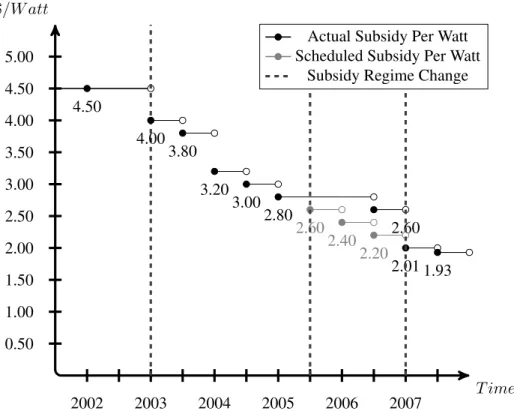
Figure 2.1 illustrates the three subsidy regimes that occur during the sample period. The vertical axis represents the subsidy rate in dollars per watt installed. The horizontal axis is the years covered during the sample period and are represented in 6-month intervals. The vertical dashed lines represent a change in the subsidy regime. The first vertical dashed line on January of 2003 represents the beginning of the first 6-month period of the second subsidy regime. The second dashed line at July of 2005 represents an unscheduled change in the subsidy rate during the second subsidy regime. The third dashed line at January of 2007 represents the beginning of the first 6-month period of the third subsidy regime. The step function represents the subsidy rate for a
T ime
$/W att
2002 2003 2004 2005 2006 2007 0.50
1.00 1.50 2.00 2.50 3.00 3.50 4.00 4.50 5.00
4.50
4.00 3.80
3.20 3.00
2.80
2.60 2.01 1.93
2.60 2.40
2.20
Actual Subsidy Per Watt Scheduled Subsidy Per Watt
Subsidy Regime Change
Figure 2.1: Subsidy Rates over Time
6-month period. The solid circles identify the beginning period of the rate and hollow circles identify the expiration of the rate. For example in Figure 2.1 the second step begins on January 1, 2003, with a solid circle, at a rate of $4.00 per watt and the rate ends on June 30, 2003 shown by the hollow circle. The next subsidy rate of $3.80 per watt begins on July 1, 2003 and expires on December 31, 2003. The black circles identify subsidy rates that actually occurred during the time period specified and the gray dots identify subsidy rates that were scheduled but never realized.
The first subsidy regime begins in 2001 with a fixed subsidy rate of $4.50 per watt. This rate remains unchanged until the end of 2002 when the regime expires. During the regime, subsidies reduce the price of an average solar panel system by 46%, decreasing the price by $19,000. The second subsidy regime begins in 2003 and continues through the end of 2006. The regime begins with an initial rate of $4.00 per watt, and decreases $0.20 semi-annually with an additional $0.40 decrease in January of 2004.5 In spring 2005, the CEC released a revision to the 2003 public
5In Figure 2.1 and 2.2, subsidy rates after 2005 in gray illustrate the proposed schedule from the 2003 public
guidebook that suspended the scheduled subsidy decrease and held the January 2005 subsidy rate of $2.80 fixed for an additional year. In July of 2006, the subsidy rate incurred the scheduled $0.20 decrease before the regime ended in December. The suspension of the scheduled decrease generated a $0.40 per watt difference in the subsidy rate relative to the original schedule. This difference reduced the price of an average solar panel system by an additional 5% or $1,500. After the second subsidy regime, the distribution of funds specific to solar panel installations was handed over to the new California Solar Initiative (CSI).
The California Solar Initiative is the third subsidy regime in the sample. The CSI begins in 2007 with a $2.01 subsidy rate6 and is scheduled to actively provide subsidies until 2016. The CSI program introduced a new system for the timing of subsidy rate changes and the conditions under which they transition. Subsidy rates are set at the state level following a rate schedule, but the transition between rates occurs at the utility region level. In 2007, all utility regions start at the same rate in the subsidy schedule.7 The transition between subsidy rates is a function of the total amount of solar electricity generated in the utility region and a region-specific level of total generation to trigger the transition.
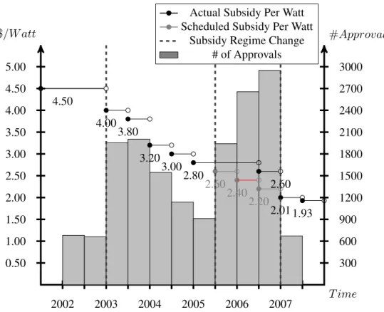
In Figure 2.2 the subsidy rate step function is overlaid by the number of installations in the sample period. The right-most vertical axis represents the number of installations and the height of the vertical gray bars correspond to the number of installations in each 6-month period.
I hesitate to make causal claims about purchasing patterns by focusing solely on the subsidy rates, and instead I discuss interesting patterns that emerge from the data. In general, the subsidies seem to be generating a response from households in the population. For the first half of the second regime, quantity demand is decreasing as subsidy rates fall. As a naive observation, quantity demanded is expected to fall as subsidies decrease and prices remain the same. During this period, the market price of a solar panel system is decreasing but at a rate slower relative to the decrease in subsidies. This results in the net price per watt for a solar panel system increasing from 2002
6Inflation-adjusted subsidy rate.
T ime
$/W att #Approval
2002 2003 2004 2005 2006 2007 0.50
1.00 1.50 2.00 2.50 3.00 3.50 4.00 4.50 5.00
300 600 900 1200 1500 1800 2100 2400 2700 3000
4.50
4.00 3.80
3.20 3.00
2.80
2.60 2.01 1.93
2.60 2.40
2.20
Actual Subsidy Per Watt Scheduled Subsidy Per Watt
Subsidy Regime Change # of Approvals
Figure 2.2: Subsidy Rate and Number of Installations Per Period
through 2005. Additionally, households know the schedule of subsidy rates within the regime and given their expectation about future prices the expected change in the net price per watt of a solar panel system is positive and increasing. Both the increase in the level of the net price per watt and the expected positive change in net prices between periods lowers the probability of purchase for households in the market. It is not surprising to see quantity demanded decreasing during this period.
A second feature of Figure 2.2 is the increase, for the remainder of the regime, in quantity demanded following an unscheduled change in the subsidy rate in 2005. At the onset of the delay, quantity demanded almost doubles.8 The delay in the scheduled decrease of the subsidy impacts per period net prices as well as households expectations about the change in net prices. Also, the increase in quantity demanded occurs three periods from the end of the second subsidy regime. In the data, there is evidence of a positive correlation between the number of periods left in a regime
8In Figure 2.2, quantity demanded doubles after the second vertical dashed line. During the first 6-month period
T ime
$/W att
2002 2003 2004 2005 2006 2007 0.10
0.20 0.30 0.40 0.50 0.60 0.70 0.80 0.90 1.00
0.91 0.85
0.82 0.81
0.43
0.46 0.47 0.67
0.58
Average Tax Credit Per Watt Tax Credit Regime Change
Figure 2.3: Average Tax Credit Per Watt
and quantity demanded, likely due to the uncertainty regarding future subsidies. Both features of the market would contribute to the increase in quantity demanded during this time period.
Tax credits are offered during the sample period in addition to the CEC subsidy program. Tax credits are intended as a secondary source of subsidy. The amount of credit a household receives is calculated from the net price of a system after accounting for the CEC subsidy. There are three tax credit regimes that overlap with the sample period. The regimes differ by rate schedule and the maximum allowable credit.
federal tax credit increased the rate to 20% of the net price but capped the maximum total tax credit at $2000. In all instances, households were provided with $2000 in federal tax credits.
Due to the structure of the tax credits, the credit per watt varies across capacities and Metropoli-tan Statistical Areas (MSA). The variation across capacity occurs as a result of net price varying across capacity. Similarly, variation in net prices across MSAs generate variation in the credit per watt received by a household. In Figure 2.3, I show the average tax credit received for each 6-month period during the sample. The vertical axis represents the tax credit per watt and the hor-izontal axis is the sample period discretized into 6-month bins. The step function represents the average tax credit for each period.
During the first regime, average credits range from $0.91 per watt to $0.81 per watt. The decrease in the credit per watt over the period reflects the decrease in the net price of a system occurring at the same time. In the second regime, the tax credit is reduced by 50% with the credit per watt starting at $0.43 per watt and increasing to $0.47 per watt. In the third regime, the credit per watt increases to $0.67 per watt. The standard deviation of the average tax credit per watt varies over the sample period. The largest variation occurs during the third regime because all households receive a fixed tax credit regardless of the capacity of the solar panel system installed. This results in larger capacity systems receiving a lower per watt tax credit.
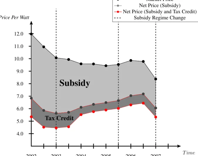
In Figure 2.4, I show the evolution of prices for a medium size (2.72kW) solar panel installation in the San Francisco area during the sample period. The vertical axis represents the price per watt for a solar panel system, and the horizontal axis represents time in 6-month periods starting in 2002 and ending in 2007. Each time period has three prices represented on the graph. The black dot represents the market price for the solar panel system during the 6-month time period. The dark gray dot represents the net price of the system after accounting for the subsidy. The red dot represents the net price of the system after accounting for the subsidy and tax credit.
T ime
Price Per Watt
2002 2003 2004 2005 2006 2007
4.0 5.0 6.0 7.0 8.0 9.0 10.0 11.0 12.0
Subsidy
Tax Credit
Market Price Net Price (Subsidy)
Net Price (Subsidy and Tax Credit) Subsidy Regime Change
CHAPTER 3 MODEL
3.1 Households’ Problem
At the beginning of the sample, no households in the market own a solar panel system. During each period, households face the decision to purchase a solar panel system or postpone purchase. Households that postpone purchase continue to be active in the market during the following pe-riod. Households that purchase are removed from the market permanently and receive a stream of benefits for the lifetime of the system. Households are constrained to purchase at most one system per period and at most one system during their lifetime. Households do not have access to a resale market, and are unable to upgrade the system after installation.1
The market is populated by a set of householdsi ∈ {1,2, . . . , N}making purchasing decisions in an infinite-horizon discrete-time framework. A household evaluates the alternatives, sit, from
the set of capacities available in the market. The full choice set of products and capacities is large and as a simplification the choice set is aggregated to five options. The choice set includes the outside option of not purchasing and four solar panel systems differentiated by capacity rating and
1The decision to constrain households to one purchase per lifetime is backed by the combination of empirical
represented by the setS, where
S =
0 Outside Option 1 Small
2 Medium 3 Large 4 Extra Large
In the choice set, zero represents the outside option of not purchasing and options one through four represent small (1.80kW), medium (2.72kW), large (4.14kW), and extra large (6.51kW) capacities. Capacities are time invariant, I discretize the distribution of capacities over the sample period into quartiles with support of zero to 10kW, the maximum allowable system capacity. I set the mean of each quartile to represent the capacity rating for each option in the choice set.
At the beginning of each period, households have full information about the current period’s state spaceΩt = {Pte, P
sp
t , Zt, S, t, τt}. The state space includes the vector of electricity prices, Pe
t; the vector of solar panel system prices, P sp
t ; the vector of product characteristics, Zt; the
set of capacities, S; the vector of taste shocks, t; and the vector of tax subsidies and credits, τt.
Households are assumed to know the distribution of the state variablesG(Ωt+1|Ωt). Households
select an alternative each period from the choice set to maximize their expected lifetime utility. Initially, the market contains all households and is defined as M1 = N. At the end of each
period, the market is adjusted to account for households that purchase. The next period’s market size is equal to,Mt+1 = Mt−Pi∈Mt1 (sit6= 0), the market size at the beginning of the period
minus the number of households that purchase in the same period. Including the endogenous change in the size of the market eliminates the potential bias discussed below.
participants to reduce potential bias on the price coefficients. The bias enters by leaving a growing set of households in the market that are perfectly price inelastic and due to their non-responsiveness to price changes put downward pressure on the parameter estimates for price. To remove the bias, I track the number of households that purchase and leave the market and adjust the market size after each period.
3.2 Utility From Purchase Let ωt = {Pte, P
sp
t , Zt, S, τt} represent the state variables without the household-level taste
shocks,t. The indirect lifetime utility from purchasing a solar panel system of sizesat timetis:
Uist(ωt, t;θ, α) = θ1+θ2ln[P Vist(peit;δ)] +θ3izt−αiln((pspist−τst)qs) +θ4M SAi +ist (3.1)
The indirect utility function is comprised of the present value from purchase, non-price product characteristics, the net price after receiving subsidies and tax credits, a MSA level fixed effect at the time of purchase, and a purchase shock that is assumed to be distributed iid Type I extreme value. The details of each part of the utility function are discussed below.
The second term in the utility specification, P Vist, represents the present value of electricity
generated over the lifetime of the solar panel system for householdipurchasing productsduring periodt. I define the present value as:
P Vist(peit;δ) =
∞
X
k=t
h
βk−t(1−δsp)k−t(1 +δe)k−tpeitqshsuni
i
(3.2)
where the bracketed term is summed over the lifetime of the system, and includes the following components:
• peitthe price of electricity for householdi
• qsthe capacity of solar panel systems
• hsuni the hours of sunlight for householdi
• δeescalation rate for electricity prices
• δsp capacity rating degradation rate
On the right hand side of Equation 3.2, the termpeitqshsuni is the flow of revenue received each
period for the generation of solar electricity. The revenue term consists of the product of the price of electricity for householdiat timet,pe
it, and the total amount of solar generated electricity during
periodt. The amount of solar generated electricity is calculated as the product of the capacity of systems,qs, and the average hours of sunlight householdireceives,hsuni , over a 6-month period.
The present value is calculated by adjusting the revenue stream each period to account for the decrease in electricity generation due to the degradation of the system, changes in future electricity prices, and discounting future income.
I calculate a constant degradation rate for solar panel systems during the sample based on data from manufacturer-provided warranties. I assume the calculated rate to be a constant percentage decrease in the production capabilities of the system and is consistent with the guaranteed produc-tion listed in the warranty. In the present value equaproduc-tion, the degradaproduc-tion rate is represented as
δsp ∈ (0,1)and reduces solar electricity generation byδsp%each period. Including the
degrada-tion rate helps improve the approximadegrada-tion of the present value of owning a solar panel system by accounting for the eventual reduction in the generation of electricity. The reduction in capacity decreases the quantity of electricity produced and leads to a reduction in revenue. Similarly, the evolution of electricity prices must be accounted for in the revenue equation.
calculate the present value of purchasing a solar panel system, and use an inflation-adjusted aver-age escalation rate calculated by the U.S. Energy Information Administration (EIA).2 Lastly, all households in the sample are assumed to discount future income by a rate ofβ.
In Equation 3.1, the third term, θ3izt, captures the effect of non-price product characteristics
on the households decision problem, specifically the efficiency rate of a solar panel system. The parameter enters the utility specification linearly and expands to include rooftop space as a di-mension of observable consumer-level heterogeneity. I discretize the distribution of rooftop space in the sample into three bins that represent small, medium, and large rooftop space households.3 I normalize the parameters relative to large rooftop space households. I interact the non-price product characteristic covariate with the additional parameters designating both small and medium rooftop space households.
θ3i =θ31+θ321
xroofi =small+θ331
xroofi =medium (3.3)
The first term in the Equation 3.3 captures the mean preference for efficiency rates in the sample population of large rooftop space households. The second and third term capture the additional utility received by households with either small or medium roof space. The decision to interact efficiency rates and roof space is best understood when considering the importance of physical area at an installation site.
Consider a household with roof space of 50 square meters. Given rooftop space and efficiency rates at the beginning of the sample, the household is constrained physically to installing a solar panel system no larger than 5kW. By the end of the sample period, the average efficiency rate increases by 30%, and the largest capacity rating for the same installation site increases to 6.5kW. The innovation in the efficiency rate over the sample period increases the semi-annual flow benefit from purchase by $200 leading to a total increase of $4000 in the present value of purchase. The
2In Figure 4.1 the electricity rates are shown for each major utility company over the sample period. Additionally,
a trend line is added that represents the escalation rate for electricity prices.
improvement in the present value of purchase from the larger capacity system may incentivize the household to delay purchase until efficiency rates are sufficiently high.
In Equation 3.1, the fourth term is the natural log of the net price of a solar panel system. The total net price per watt is comprised of the market price per watt,pSP
ist, subtracted by the approved
subsidy per watt and tax credit per watt,τst for householdiand capacity sizesat timet. The total
net price of a solar panel system is calculated as the product of the total net price per watt and the capacity,qs, for choices.4 The coefficient αi on the net price captures the disutility from the net
price of a solar panel system.
As a starting point, I discretize the distribution of housing values, at the state level, into terciles and assign each household in the sample population to a housing value bin. The bins represent low, medium, and high value homes, and serve as a proxy for wealth in the utility specification. The price coefficientαiin Equation 3.4 includes additional parameters interacted with an indicator
function identifying a household’s housing value. By including αi, I introduce an observable
measure of household-level heterogeneity in the estimation of price responsiveness.
αi =α1+α21(xivalue=medium) +α31 xvaluei =high
(3.4)
I estimate the disutility from log prices in the sample population for households in the low housing value category with theα1 coefficient. I estimate the differences in disutility that households of
medium and high value receive from the net price with the parametersα2 andα3.
The next term, θ4MSAi, is a Metropolitan Statistical Area (MSA) level fixed effect received at
the time of purchase. I include an MSA-level fixed effect in the model to reduce the presence of endogeneity from omitted variables that are correlated with covariates in the model. Some examples of this might be the average environmental preferences within a MSA, advertising or marketing for solar panel subsidies, or pollution levels within a MSA.
In areas that are more ”green” or environmentally friendly households might receive additional
4It is important to note that while capacity is time invariant, the total net price per watt varies over time by the
social utility from installing a solar panel system that is not accounted for in the current specifi-cation. The unobserved social benefit from installing solar panels could be correlated with prices making price endogenous in the model. The MSA fixed effect is included to capture variation from a time invariant MSA level preference for green products and the social utility associated with it. Another potential source of variation is advertising or marketing for either the solar panel subsidies or solar panel installations in general. Lastly, MSA level characteristics that are correlated with clean energy, level of pollution in the MSA, could generate endogeneity issues in the model. For example, a household in L.A., where pollution is persistently high, might purchase a solar panel system and receive unobserved utility from the belief that the system will help reduce pollution in the local area and provide positive externalities to the community.
3.3 Utility From Waiting
In markets with durable goods, capturing the option value of waiting is important in explain-ing the choice behaviors observed by households (Melnikov 2001, Gowrisankaran and Rysman (2012)). The option value of waiting is the expected utility from participating in a future market. The household choice-specific value function for choosing not to purchase is represented byVi.
Vi(ωt, t;θ, α) =δif0t+i0t+β
ˆ
ωt+1
ˆ
t+1
Vi(ωt+1, t+1;θ, α)G(ωt+1, t+1|ωt, t)dωt+1dt+1
(3.5) The contemporaneous indirect utility from not purchasing is characterized by a flow utility, δfi0t, that is normalized to zero and an additive preference shock, i0t. The last term on the right hand
side of Equation 3.5 represents the option value of waiting, and is integrated over the conditional joint distribution of the state variables,G(ωt+1, t+1|ωt, t). Intuitively, the term captures the mean
utility a household expects to receive by waiting to purchase considering future prices, technology, subsidies, tax credits, and preference shocks.
know the distribution of their future preference shocks and are able to integrate over them. House-holds are assumed to believe that the price per watt for solar panel systems follow a Markovian process. Specifically, households expect that the price per watt for a solar panel system follows a first order autoregressive specification,
PitSP+1 =δi1+δi2PitSP +µit+1 (3.6)
whereµit+1is normally distributed iid shock with mean zero and varianceσsp2 . The autoregressive
parameterδi2 satisfies the condition for stationarity0< δi2 <1,∀i.
In Equation 3.6, I allow for the pricing process to differ across MSAs and allow local market conditions to influence households expectations about future prices. A vast majority of installations occur by local installers within the MSA and as such markets can be treated separately. Changes in local market demand and supply conditions should generate differences across MSAs in the pricing process to the extent that markets are independent. I compare the results of the per MSA estimation of Equation 3.6 to a state-level pricing process, in which I assume that households believe that solar panel system prices evolve similarly across capacity and MSA.
3.4 Tax Policies
Over the three subsidy regimes, information regarding policy changes becomes publicly avail-able only at the time of the change. The uncertainty households have regarding future subsidy regimes and changes to rate schedules creates uncertainty that enters into the dynamic choice problem. Household beliefs regarding future regime changes can generate anticipatory behavior. Anticipatory behavior has been shown to impact the effectiveness of a regime change (Mertens and Ravn, 2010; Crepon et al, 2010, Blundell et al. 2014). To examine this, I specify deterministic cases that vary by household beliefs regarding the existence and rate schedule of a future regime. The deterministic cases are a simplistic way to capture anticipation effects that might arise from beliefs about future regimes and control for them in estimation.
T ime
$/W att
2002 2003 2004 2005 2006 2007
0.50 1.00 1.50 2.00 2.50 3.00 3.50 4.00 4.50 5.00
4.50
4.00 3.80
3.20 3.00
2.80
2.60 2.011.93 Actual Subsidy Per Watt Subsidy Regime Change
Figure 3.1: Case 1: Perfect Foresight
describe the cases, let P r(τ0|τ) be defined as the probability that future regimeτ0 occurs condi-tional on the household being in subsidy regimeτ. Note that all households in the population are assumed to share the same beliefs regarding future regimes.
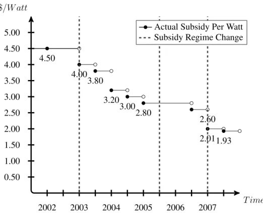
In the first case, I assume that households have full information about all regimes, and can predict the future perfectly. Perfect foresight implies that households have the following beliefs
P r(τ0|τ) =
1 ifτ0 =τtrue
0 Otherwise
(3.7)
whereτtruerepresents the true future subsidy regime. Figure 3.1 illustrates the information
In the second case, I assume that all households are pessimistic and believe that no additional subsidies are offered after the expiration of the current regime. Pessimism implies that the discrete probability density function takes the following form
P r(τ0|τ) =
1 ifτ0 = 0 0 Otherwise
(3.8)
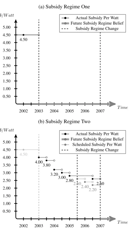
where households believe with probability one that no future subsidy regimes will exist. In Figure 3.2a, I show a household’s belief regarding the existence of a future regime conditional on being in the first regime of the sample period. When a new subsidy regime is reached the household updates their information about the new policy but retains the same beliefs about the existence of a future subsidy. In Figure 3.2b, I illustrate the transition to the second subsidy regime and how the belief regarding a future regime does not change. The beliefs enter the households’ problem through the expectation of future prices, and is expected to decrease the option value of waiting relative to the perfect-foresight case.
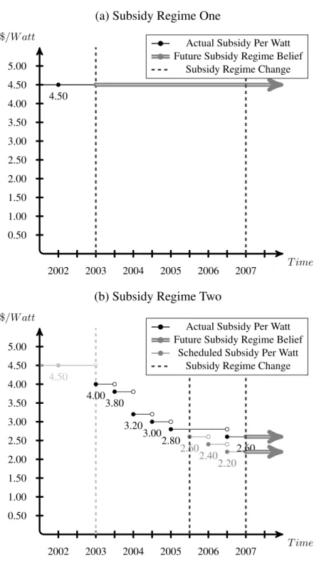
In the third case, auto-renewal, households believe that the final subsidy rate in the present regime will continue after the regime expires. Auto-renewal implies that the discrete probability density function takes the following form
P r(τ0|τ) =
1 ifτ0 =τf
0 Otherwise
(3.9)
where τf represents the final rate in the current subsidy regime τ. In Figure 3.3a, I illustrate a household’s belief about future subsidies conditional on being in the first subsidy regime. I show in Figure 3.3b how the belief about a future regime does not change when a new regime is enacted but the future subsidy rate is updated.5
5In Figure 3.3b I use two gray arrows to illustrate beliefs about a future subsidy regime. The top gray arrow
(a) Subsidy Regime One
T ime
$/W att
2002 2003 2004 2005 2006 2007
0.50 1.00 1.50 2.00 2.50 3.00 3.50 4.00 4.50 5.00
4.50
Actual Subsidy Per Watt Future Subsidy Regime Belief
Subsidy Regime Change
(b) Subsidy Regime Two
T ime
$/W att
2002 2003 2004 2005 2006 2007
0.50 1.00 1.50 2.00 2.50 3.00 3.50 4.00 4.50 5.00
4.50
4.00 3.80
3.20 3.00
2.80
2.60 2.60
2.40 2.20
Actual Subsidy Per Watt Future Subsidy Regime Belief
Scheduled Subsidy Per Watt Subsidy Regime Change
3.5 Identification
The identification strategy presented is fairly standard and follows the dynamic consumer de-mand literature closely. Generally, changes in the market share of a product s associated with a change in a product characteristic of good s helps identify the mean utility from a character-istic. The identification of the parameter on price, present value of purchase, and technological innovation are discussed below in detail.
The coefficients on the net price of a solar panel system are identified by variation in uptake that are associated with variation in the net price. Specifically, identification of the vector of parameters
αicomes from variation in purchasing behavior within each tercile of the housing value distribution
that is associated with variation in the net price. Variation in the net price over time of solar panel systems occur through three channels that are exogenous to the households choice problem. First, the price of solar panels depends on a global market and price variation comes from exogenous market forces: inputs for production (e.g. variation in the price of silicon), technological shocks to the production process, and global demand for solar panels. Second, the price of installing a solar panel system varies due to changes in installation costs for the installer such as: learning by doing (e.g. returns to experience), technological innovation with respect to mounting equipment, and economies of scale. Third, subsidy rates and tax credits vary over the sample period supplying an additional layer of exogenous price variation.
Variation in purchase related to variation in the present value of purchase over time identifies the parameterθ2. The present value of purchase varies over time through changes in the average
price of electricity. The price of electricity varies over time based on regulatory agencies’ decisions at the utility level, regional demand for electricity, and input costs.
The vector of parametersθ3ion the non-price product characteristic, efficiency rate, is identified
CHAPTER 4 DATA
I assemble a new dataset from a variety of sources to estimate the model in Chapter 3. I use choice data from the California Energy Commission’s (CEC) Emerging Renewable Program that covers eight years of residential solar panel installations in the state of California. I expand the choice data by collecting detailed housing and solar panel characteristic data for each observation in the CEC dataset. I pair these with relevant datasets that include measures of usable sunlight hours and electricity prices during the sample period. To complete the panel, I simulate households that are active in the solar panel market but do not purchase during the sample. The following section discusses each of the above points in detail.
The CEC data track all households who purchase a solar panel system and receive a tax subsidy from 1998 through 2006. These data include the address of the residence, capacity of the system installed, total price paid, subsidy received, make and model of the installed solar panel system, subsidy approval date, installation completion date, and the utility region in which the household is located. I drop the first three years of data due to missing information and low numbers of purchase during that time period. Additionally, I drop both commercial and utility-scaled installations and keep purchases made by residential households. Lastly, I drop observations where the price per watt is below $4.00 or greater than $30.00.1 This results in a dataset that consists of 12,736 observations of purchase for the sample period of 2002 through 2006.
I expand the data from the CEC by adding housing characteristics for each purchaser. I collect the housing characteristics by matching the physical address of the purchaser with the real estate website Zillow.com and scrape the relevant information. For each purchaser, I retrieve information
1A report by the CEC, Wiser, Bolinger, Cappers, and Margolis (2006), discusses how these are most likely input
on the value of the home, number of stories, square footage, number of bedrooms, and year built.2 As a redundancy check, I perform a similar task but with an alternative data source, Trulia.com, and match housing characteristics with address information.
In Table 4.1, I present descriptive statistics specific to households that purchase during the sample. The columns of the table are separated by geographic region. The first column shows de-scriptive statistics for all purchasers at the statewide level. The second through the fifth column are separated by MSA: 1) Los Angeles-Long Beach-Riverside, 2) San Francisco-San Jose-Oakland, 3) San Diego-Carlsbad-San Marcos, and 4) Fresno-Madera-Sacramento.3 The San Francisco-San Jose area has the highest average home values at $841,070 with the coastal MSAs, Los Angeles and San Diego, following with an average home value of $560,000. The more in-land region, Fresno and Sacramento, have the lowest average housing value at $373,066.
The San Francisco metropolitan statistical area makes up 47% of the total number of purchases in the data with 5986 solar panel system installations. Purchasers in San Francisco have the small-est average roof space at 183.49 m2 and install smaller than average capacity systems, 3.54kW,
relative to the rest of the state. Also, purchasers in San Francisco buy slightly earlier in the sample, on average, and pay higher prices per watt for the systems. The descriptive statistics suggest that a higher share of early adopters of solar panel systems live in the San Francisco area.
I simulate the population of households for each zip code in the CEC dataset. The simulated households are generated using a dataset from Dataquick. The data include marginal distribution information at the zip-code level that describes housing characteristics of potential market partic-ipants.4 The data characterizes households within each zip code by five housing characteristics: housing value, the number of stories, square footage, the number of bedrooms, and the year the house was built. For each characteristic, the dataset includes the first two moments of the marginal
2Zillow.com uses an algorithm for housing value named Zestimate that considers recent sales of similar homes and
neighborhood characteristics when estimating the housing value.
3It is important to note that not all zip codes within the MSAs are represented in Table 4.1. I drop all zip codes
with less than 5 purchases during the sample period. The result is a total of 345 zip codes used in estimation.
4This includes single family homes, both detached and attached. Multi-family homes such as condominiums and
distribution, number of observations, correlations between the housing characteristics, and the quartiles of the marginal distribution. The matrix of correlations between housing characteristics provides useful information by improving the accuracy of the simulated populations.
I use a copula function to create a joint distribution of housing characteristics and simulate the entire population of households in each zip code. The copula function is assumed to be multivariate normally distributed (Gaussian Copula) with mean zero and a covariance-variance matrixΣ. The matrixΣis calculated using the correlation measures between characteristics and the variance of each characteristic. Zip codes are independently simulated using a multivariate normal copula with each zip code having a uniqueΣmatrix.
The copula function creates a joint distribution of household characteristics from a set of marginal distributions. The Gaussian copula provides structure by enforcing the correlations that exist between the housing characteristics when simulating households.5 The result is a simulated population of households characterized by a vector of discrete housing characteristics from a nor-mal distribution.
I merge the simulated dataset and the set of purchasers by matching housing characteristics. For each zip code, I search the simulated dataset for a vector of housing characteristics that match identically with the vector of housing characteristics for each purchaser. Once a match is found, I replace the simulated household with the matched purchaser. The process is performed for all purchasers and across all zip codes represented in the sample. This results in a dataset of 2,272,841 households in the market for residential solar panel installations that includes both households that purchase and do not purchase during the sample period. With over 2 million households participating in the market for solar panel systems and only 12,736 purchases during the sample, the size of the choice probabilities are a potential concern in estimation. To improve the choice probabilities, I reduce the market size for each MSA informed by a survey conducted in California about attitudes toward renewable energy.
In 2001, an independent study was contracted by the California Energy Commission, con-ducted by Marylander Marketing Research, with the stated purpose of determining awareness and attitude toward renewable energy sources among households and businesses in California. In the survey households were asked several questions regarding their history with renewable energy sources, knowledge of renewable energy, and their desire to have a renewable energy source at their residence.
The question of interest for reducing the market size asked households the following question: What is the likelihood of installing a solar, wind, or fuel cell renewable energy system at your home?
1. Definitely Would Install 2. Probably Would Install 3. Might or Might Not Install 4. Probably Would Not Install 5. Definitely Would Not Install
The survey finds that, conditional on not ever owning a renewable energy system, 15% of the population answered either definitely or probably would install, 23% said they might or might not install, and 62% answered that they either probably or definitely would not install. The large share of households answering negatively suggest a reduction in the population of market participants is appropriate during the sample period.
used in estimation.
Outside of housing characteristics, households face location-specific exogenous characteristics in the form of electricity prices by utility region and the number of hours of sunlight at their residence. The data on electricity prices originates from the websites of the three largest utility companies in California: Pacific Gas and Electric (PGE), Southern California Edison (SCE), and San Diego Gas and Electric (SDGE). These three utility companies supply electricity to over 85% of all households in California and more importantly provide electricity to the zip codes in the sample. Within all three utility companies, there is a menu of electricity rate plans that households can choose from. The plans are based on either baseline quantity-tiered pricing or time-of-use pricing. I am not able to take advantage of the detailed pricing data without information on the type of plan a household chooses and their consumption of electricity. Instead, I use a dataset from the California Public Utility Commission (CPUC) that calculates average prices for residential electricity consumption for each utility region over time.6
In Figure 4.1 the electricity price per kilowatt hour is represented on the vertical axis and the horizontal axis represents time, beginning in 2002 and ending in 2010. The electricity prices are deflated to 2006 price levels with rate changes only occurring annually.7 Average electricity prices are generally increasing over the time period. The relatively high prices in 2002 are a residual effect from the deregulation of electricity markets that occurred in the late 1990s and early 2000. San Diego Gas and Electric have the highest electricity prices throughout the time period shown. Average electricity prices are similar between Pacific Gas and Electric and Southern California Edison, but PGE prices tend to be slightly higher.
I gather data for the number of hours of sunlight a household receives from the National Re-newable Energy Laboratory’s (NREL) Typical Meteorological Year (TMY3) dataset. The data are collected by 74 weather stations located across California that record a variety of meteorological measures. Using the data, I aggregate from a hourly measure of sunlight to a 6-month measure.
T ime
Cents Per kWh
2002 2003 2004 2005 2006 2007 2008 2009 2010 13.0
13.5 14.0 14.5 15.0 15.5 16.0 16.5 17.0 17.5
Cents Per kWh PGE Cents Per kWh SDGE
Cents Per kWh SCE End of sample period
I average the semi-annual hours of sunlight over the years during the sample to create a time in-variant measure of the average number of hours of sunlight a location receives. The geographical longitude and latitude of each station is differenced with the latitude and longitude of the center of each zip code, and the station closest to the zip code is used to measure sunlight hours.8 An-nual average sunlight hours are presented in Table 4.1 across the state and for each MSA. There is substantial variation in annual sunlight across the MSA regions with an average of 1820.29 hours of sunlight and a standard deviation of 93.83 hours. The least amount of sunlight occurs in the San Francisco region where the average is 1757.18 hours of sunlight. The largest amount of sun-light occurs in the Los Angeles region where the households receive an average of 1920.55 hours of sunlight annually. On average households in California receive 5 hours of usable sunlight per day. The difference between the hours of sunlight received in San Francisco and Los Angeles is approximately 32 days of average sunlight.
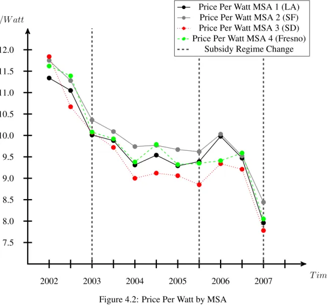
Households choose over a set of solar panel systems that vary by capacity, price, and technol-ogy. The data on solar panel system capacity and price are included in the CEC dataset and are shown in Table 4.1 above. While the average total price of a solar panel system is similar across MSAs there is variation in both the capacity of the system installed and the price per watt. In Figure 4.2 the average price per watt of a solar panel system is shown by MSA over the sample period. At the beginning of the sample prices are closely matching but after 2003 the gap between the average prices increases. The largest gap shows up between San Francisco and San Diego where at one point they differ by $1 per watt installed.
The aggregation of price per watt into an average for all installations is a bit misleading. Figure 4.3 displays the price per watt within the Los Angeles MSA by capacity bin and over the sample period. The figure shows evidence of size discounting occurring in the solar market. I find that extra-large capacity systems have significantly lower prices per watt relative to small capacity solar panel systems. There is almost a $2.00 price per watt difference between the small capacity installations and extra large capacity installations during 2005. Note that prices seem to trend
8The distance is taken using using the haversine formula. The haversine formula is an equation that finds the
T ime
$/W att
2002 2003 2004 2005 2006 2007
7.5 8.0 8.5 9.0 9.5 10.0 10.5 11.0 11.5 12.0
Price Per Watt MSA 1 (LA) Price Per Watt MSA 2 (SF) Price Per Watt MSA 3 (SD) Price Per Watt MSA 4 (Fresno)
Subsidy Regime Change
Figure 4.2: Price Per Watt by MSA
similarly over time both across capacity bins and across MSAs. Also, there is a growing difference in the price level of solar panels systems over time.
A solar panel system is a collection of solar panels joined together to generate an output of electricity. The characteristics of a solar panel system depends directly on the characteristics of the solar panels in the group. In the CEC dataset all households purchase a solar panel system that is a collection of one unique solar panel. Solar panel system characteristics are created by collecting non-price product characteristics for each brand and model combination of solar panels observed in the CEC dataset.
T ime
$/W att
2002 2003 2004 2005 2006 2007
7.50 8.00 8.50 9.00 9.50 10.00 10.50 11.00 11.50 12.00
Capacity Bin 1 (Small) Capacity Bin 4 (X-Large)
Subsidy Regime Change
rating, efficiency rate, physical size, type of panel, warranty information, and additional technical details for a specific solar panel.9 Two tables are included to show the distribution of characteristics in the full sample of solar panels and the more restricted sample used in estimation. The full set of unique solar panels is shown in Table 4.4 and the set of panels that result from constraints imposed on the purchase data are represented in Table 4.5.
The two tables show the narrowing of the solar panel market after imposing restrictions on geographic location, total capacity of the system, and measurement error in reporting of prices. The market for residential solar panels is different relative to the entire market. First, average PTC capacity rating per panel is 40kW less in the residential market relative to the entire market.10 Also, the maximum capacity rating of a solar panel in the residential market is 297kW where in the broader market the maximum capacity rating of a solar panel is 779.8kW. The physical size of an average solar panel in the residential market is smaller both in physical area, 1.22m2 versus
1.49m2 in the larger market, and weight, 15.44 kg versus 18.12 kg in the broader market. Lastly,
average efficiency rates in the residential market are less relative to the broader market with close to a 9% difference in the efficiency rate. The findings suggests that the broader market for solar panels is not the appropriate choice set for residential households. Instead, the characteristics of solar panel systems used in estimation are constrained to the restricted sample.
I capture innovation in solar panel technology through the improvement in efficiency ratings of solar panels over the sample period. In Figure 4.4 average efficiency rates are shown over time. The vertical axis represents efficiency rates in percentage terms with an average efficiency rate of 10.46% at the beginning of the sample period. Over the sample, efficiency rates are trending upwards and increase a total of 29% from 2002 to 2007.
9A sample of a specification sheet is included in appendix.
10The first measure of capacity is the standard test condition (STC) ratings. STC ratings are provided by the
T ime Rate(%)
2002 2003 2004 2005 2006 2007 2008
10.0 10.5 11.0 11.5 12.0 12.5 13.0 13.5 14.0 14.5
Average Efficiency Rate (%)
Variable Obs Mean Std. Dev. Min Max STC Capacity Rating 1016 189.56 69.36 14 864 PTC Capacity Rating 1016 169.69 63.24 11.8 779.8 Efficiency Rates 1016 11.67 2.19 2.35 18.48 Panel Area (m2) 1016 1.49 1.09 .12 18.59
Panel Depth (mm) 972 43.89 13.18 2.5 213
Weight (Kg) 967 18.12 6.99 1.9 67
Table 4.4: Full Set of Solar Panels
Variable Obs Mean Std. Dev. Min Max
STC Capacity Rating 271 147.61 53.21 17 330 PTC Capacity Rating 271 131.88 47.84 15.7 297 Efficiency Rates 271 10.82 2.4 2.35 16.48 Panel Area (m2) 271 1.22 .37 .35 2.43 Panel Depth (mm) 266 45.12 10.32 2.5 60
Weight (Kg) 265 15.44 6.98 2.2 48.5
CHAPTER 5 ESTIMATION
To estimate the model discussed in Chapter 3, I impose several assumptions to reduce computa-tion time and provide tractability in estimacomputa-tion. Given the assumpcomputa-tions, estimacomputa-tion of the dynamic discrete choice problem is accomplished using three-stage maximum likelihood estimation with a combination of Rust’s (1987,1994) nested fixed point algorithm (NFXP) and backwards induction to estimate the continuation value of staying in the market. The first stage of the estimation routine recovers parameters that govern the transition of solar panel system prices. Using the estimated parameters for solar panel system prices, the second stage of the estimation iterates over a nested loop. The inner loop estimates the continuation value of staying in the market and the outer loop estimates parameters through maximum likelihood estimation. The third stage corrects consistency issues with the covariance matrix of second-stage parameter estimates by using the consistent esti-mate of the parameter vector from the first two stages to maximize the full log-likelihood equation. Altogether the three stage algorithm is able to estimate the dynamic discrete choice problem and generate consistent parameter estimates. The details of the assumptions, algorithm, and calculation of standard errors are discussed in what follows.
The Bellman equation representing the household’s per period maximization problem is framed as a decision between purchasing one of four available products in the market or choosing to forgo purchase and take the continuation value of staying in the market for an additional period. From chapter 3, the household’s maximization problem is modeled as:
Vit(ωt, t;θ) =max{i0t+β
ˆ
ωt+1
ˆ
t+1
Vit+1(ωt+1, t+1;θ)G(ωt+1, t+1|ωt, t)dωt+1dt+1,
The first term on the right hand side of equation 5.1 represents the utility a household receives when deciding to forgo purchase and stay in the market the next period. The second term on the right hand side of the equation, Uist(ω, ;θ), represents the utility a household receives by choosing
optimally from the set of available products in the market.
In equation 5.1 the state variableωandare jointly determined from a conditional joint density functionG(ωt+1, t+1|ωt, t). By assuming conditional independence, the Bellman equation can
be rewritten to simplify the problem:1
Vit(ωt, t) = max{i0t+β
ˆ
ωt+1
ˆ
t+1
Vit+1(ωt+1, t+1)f(t+1|ωt+1)dt+1h(ωt+1|ωt)dωt+1,
maxs∈{1,2,3,4}Uist(ωt, t;θ)} (5.2)
The joint densityG(ωt+1, t+1|ωt, t)from equation 5.1 is separated into two conditional densities.
The simplification implies that: (i) given today’s state,ωt, the’s are independent over time, (ii)
conditional on today’s state,ωt, the next periods stateωt+1is independent oft.
Since the utility from purchase does not include a continuation value it is helpful at this point to focus on the utility from foregoing purchase. First, the inner-most integral is defined as:
EVit+1(ωt+1) =
ˆ
t+1
Vit+1(ωt+1, t+1;θ)f(t+1|ωt)dt+1 (5.3)
The type I extreme value distributional assumption for thetaste shocks simplifies the integral in equation 5.3 to the familiar closed form solution:
EVit+1(ωt+1) = log
" S X
s=1
e(Vit+1(ωt+1,s;θ))+e(Vit+1(ωt+1,0;θ))
#
(5.4)
The expected future utility from choosing to postpone purchase is simplified as the integration
1Rust (1994)discusses complications when estimating the model specified above, and introduces several
stan-dard assumptions to reduce computational complexity and ensure consistency. The only one discussed here is the conditional independence assumption. Conditional independence is satisfied if and only if the joint density