Honors_Thesis___CONCENTRIC_TUBE_ROBOT.pdf

LEARNING COMPLETE SHAPES OF CONCENTRIC TUBE ROBOTS

Armaan Sethi

A dissertation submitted to the faculty at the University of North Carolina at Chapel Hill in partial fulfillment of the requirements for the Honors Thesis in the Department of Computer Science in the

College of Arts and Sciences.

Chapel Hill 2020

Approved by:

Ron Alterovitz

Stephen M. Pizer

Donald E. Porter

Armaan Sethi

ABSTRACT

Armaan Sethi: Learning Complete Shapes of Concentric Tube Robots (Under the direction of Ron Alterovitz)

Concentric tube robots, composed of nested pre-curved tubes, have the potential to perform

minimally invasive surgery at difficult-to-reach sites in the human body. In order to plan motions that

safely perform surgeries in constrained spaces that require avoiding sensitive structures, the ability

to accurately estimate the entire shape of the robot is needed. Many state-of-the-art physics-based

shape models are unable to account for complex physical phenomena and subsequently are less

accurate than is required for safe surgery. In this work, I present a learned model that can estimate

the entire shape of a concentric tube robot. The learned model is based on a deep neural network that

is trained using a mixture of simulated and physical data. I evaluate multiple network architectures

and demonstrate the model’s ability to compute the full shape of a concentric tube robot with high

accuracy. The full shape of a concentric tube robot is necessary in order to plan collision free motions

First, I would like to thank my advisor, Ron Alterovitz, for mentoring me since my freshman

year and encouraging me to pursue research in robotics.

This work would not have been possible without the help and mentorship of Alan Kuntz.

Additionally, I would like to thank Chris Bowen, Jeff Ichnowski, and all the students in the Alterovitz

Lab for welcoming and supporting me.

I would like to thank my committee members for their valuable time, guidance, support, and

feedback.

This research was supported in part by the U.S. National Institutes of Health (NIH) under award

R01EB024864.

Finally, I would like to thank my family and all my friends that I made during my undergraduate

TABLE OF CONTENTS

LIST OF FIGURES . . . vi

LIST OF TABLES . . . vii

CHAPTER 1: INTRODUCTION . . . 1

CHAPTER 2: RELATED WORK . . . 3

CHAPTER 3: METHODS . . . 5

3.1 Generating Ground Truth Data . . . 5

3.2 The Neural Network Architecture . . . 6

3.2.1 Input to the network . . . 6

3.2.2 Output of the network . . . 7

3.3 Training of the Model . . . 8

CHAPTER 4: RESULTS . . . 11

4.1 Evaluation of Polynomial Basis Function . . . 11

4.2 Evaluation of Varying Network Architectures . . . 11

4.3 Accuracy Comparison to Physics-Based Model . . . 13

4.4 Speed Comparison to Physics-Based Mode . . . 15

CHAPTER 5: DISCUSSION AND CONCLUSION . . . 18

1.1 Overview Figure . . . 2

3.1 Camera Setup to Generate Ground Truth Data . . . 6

3.2 Process of Generating Ground Truth Data from Images . . . 7

3.3 Orthonormal Polynomial Basis Functions Generated Using Gram-Schmidt Orthogo-nalization . . . 8

3.4 Sample Distribution of Training Data . . . 10

4.1 Histogram of Maximum Error Along the Robot’s Shaft . . . 13

4.2 The L2 _{Distance of Points Along the Robot’s Shaft . . . . 15}

4.3 Three Examples of the Shape Our Learned Model Computes . . . 16

LIST OF TABLES

4.2 Average Learned Model Accuracy Results (Mean±Std in mm), Maximum Deviation Along Shaft . . . 12

4.3 Average Learned Model Accuracy Results (Mean ±Std in mm), Mean Squared Error Along Shaft . . . 12

Introduction

Concentric tube robots are needle diameter robots composed of nested pre-curved tubes [1]. By

rotating and translating the tubes with respect to one another, the robot’s shaft takes curvilinear

shapes. This enables these robots to curve around anatomical obstacles to perform surgical procedures

at difficult-to-reach sites. Concentric tube robots have the potential to enable less invasive surgeries

in many areas of the human body, including the skull base, the lungs, and the heart [2].

Motion planning can enable concentric tube robots to move safely through the body, reaching

desired surgical targets while avoiding colliding with sensitive anatomical obstacles, such as blood

vessels, nerves, and organs [3, 4, 5]. In order to plan safe motions for concentric tube robots that

automatically avoid unintended collisions with the patient’s anatomy, motion planning algorithms

simulate robot motion, performing collision detection to ensure that the robot’s geometry does not

collide with obstacles [6]. In order to perform collision detection, an accurate geometric model of the

robot’s entire shape is required.

Prediction of the entire shape of a concentric tube robot from its control inputs is challenging,

and current state-of-the-art shape models are often unable to accurately account for complex and

unpredictable physical phenomena such as inconsistent friction between tubes, non-homogeneous

material properties, and imprecisely shaped tubes [7, 8].

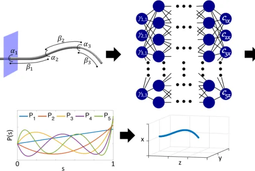
I present a data-driven, deep-neural-network-based approach that learns a function that accurately

models the entire shape of the concentric tube robot, for a given set of tubes, as a function of its

configuration (see Fig. 1.1). The neural network takes as input the robot’s configuration, and the

network outputs coefficients for orthonormal polynomial basis functions inx,y, andz parameterized

by arc length along the robot’s tubular shaft. In this way, a function representing the entire shape

of the robot can be produced by one feed-forward pass through the neural network.

The key insight behind the parameterization used by my collaborators and I is that the uncertainty

g1,1

c

c

c

c

0 0.2 0.4 0.6 0.8 1

-2 -1 0 1 2 3 4

P₁ P₂ P₃ P₄ P₅

0 1

P(

s)

s 0 50 100 150

z -100 0 100 y -100 -50 0 50 100 x

0 50 100 150

z -100 0 100 y -100 -50 0 50 100 x

0 50 100 150

z -100 0 100 y -100 -50 0 50 100 x x y z

Figure 1.1: Given a concentric tube robot configuration defined by the translations and rotations of the tubes (upper left), our neural network (upper right) outputs coefficients for a set of polynomial basis functions (lower left) that are combined to model the backbone of the robot’s 3D shape (lower right).

length of the robot’s shape, however, is independent of these and as such is generally not subject

to the same sources of uncertainty. We can leverage this known state by parameterizing our shape

function by arc length. Additionally, we leverage the machine learning technique known as transfer

learning [9]. Transfer learning allows our model to first utilize a large simulation data set to learn

the general structure of concentric tube robot kinematics and then to leverage a smaller real-world

data set to learn the differences between the simulated data and the real robot’s kinematics. We

demonstrate that pre-training our network on simulated data produced by a physics-based model

and then fine-tuning the model on real-world, sensed concentric tube robot shapes enables the model

to perform more accurately than models trained on either simulated or real-world data alone. We

can then use the model in order to significantly speed up current motion planning techniques.

Together with co-authors, I have recently published many of the contributions of this thesis

Related Work

Concentric tube robots have been shown to potentially improve patient outcomes by reducing

the invasiveness of a variety of surgical tasks [2]. However, the manual control of these devices is

extremely unintuitive, motivating research into their higher-level user interfaces to operate these

robots, such teleoperation in which a user remotely specifies a target for the robot’s tip to reach [4, 12].

Teleoperation requires some form of computational actuation of the robot, a function that has been

served by both traditional control methods and via motion planning.

Traditional control applied to concentric tube robots has primarily focused on computing controls

that are based on desired tip movements. For example, there are methods that have been developed

that compute controls based on the robot’s Jacobian [7, 13]. In addition, Fourier series based

approximations of the robot’s kinematics have been utilized for control [14]. However, these local

control methods can struggle to compute collision-free motions that require complex trajectories in

the presence of constrained anatomy.

Conversely, motion planning enables concentric tube robots to take a global view of motion

in constrained anatomy. This allows for more complex motions that avoid obstacles. In order

to accomplish this, a few approaches have been proposed. In order to enable fast computation,

simplified kinematics have been used in motion planning [15, 16]. Additionally, Sampling-based

motion planning methods for concentric tube robots have also been proposed [3, 17, 4, 12, 5].

In both cases where local control is utilized or motion planning is utilized, an accurate shape

model, mapping the control variables of the robot to its physical geometry in the world, is required.

This shape model is used in order to assure the concentric tube robot does not collide with patient

anatomy.

Other sensors, such as FBG sensors, have been used with concentric tube robots to estimate

their curvature both in bending and in torsion [18]. These methods sense the shape of the concentric

a model that can anticipate its shape in simulation prior to execution of the physical motion is

necessary. For this reason, a method that computes the shape of the robot in advance is required for

motion planning.

Most existing shape computation methods represent the concentric tube robots using the Cosserat

rod equations [19, 20] that define a system of ordinary differential equations which, when solved,

provide the shape of the concentric tube robot’s backbone. Such models have increased in complexity

over time, with the most advanced modeling physical effects such as torsion [14, 7]. Other physical

phenomena, such as friction between tubes, have been investigated but not yet fully and not yet

effectively integrated into such physics-based models [21].

Machine learning methods have been applied to both the forward kinematics and inverse

kinematics of continuum robots. For instance, the inverse kinematics of tendon-driven robots

have been computed using various data-driven methods [22] and feed forward neural networks [23].

Neural networks have also been applied to learning the inverse kinematics of pneumatically-actuated

continuum robots [24]. Neural network models have been successfully used to more accurately model

the forward kinematics and inverse kinematics of concentric tube robots [25, 26]. However, these

kinematic models only consider the pose of the robot’s tip. In order to successfully plan and execute

motions that avoid unwanted collisions between the robot’s shaft and patient anatomy, the pose of

Methods

In order to safely plan motions for concentric tube robots operating around sensitive anatomical

structures, we must be able to anticipate the shape that the robot takes in the body along its entire

length, not only at its tip, as we actuate the robot. For this reason, we consider the problem of

accurately mapping a concentric tube robotâs configuration, defined by each of its tubeâs rotations

and translations, to the robotâs geometry in the physical world. Our neural network model, trained

on a combination of simulated and sensed, real-world data, takes the robot’s configuration as input

and outputs coefficients for an arc length parameterized space-curve function that represents the

robot’s backbone. This function, combined with knowledge of the cross-sectional radii of the robot’s

tubes, represents knowledge of the robot’s shape in the world at that configuration (see Fig. 1.1).

3.1 Generating Ground Truth Data

In order to learn a shape function for the concentric tube robot, data representing the robot’s

shape as a function of its configuration must be gathered. To gather shape data, we utilize a

multi-view 3D computer vision technique called shape from silhouette [27], in which multiple images

of the robot’s shape for a given configuration are collected from cameras with known position and

orientation (see Fig. 3.1).

We place two cameras at roughly orthogonal angles around the robot such that the robot’s shaft

is in the field of view of both cameras. We then move the robot to a sequence of randomly sampled

configurations and image the robot at each configuration with both cameras simultaneously (see

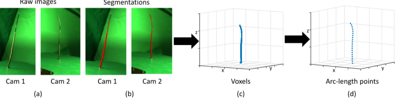
Fig. 3.2a). Then for each pair of images we automatically segment the robot’s shaft in each image

using color thresholding (see Fig. 3.2b). For each pixel in the segmentation a ray is traced out from

the camera’s position through its image plane (we calibrate the cameras’ intrinsic and extrinsic

parameters using MATLAB’s Computer Vision Toolbox). These rays then pass through a voxelized

representation of the world, and voxels that are intersected by rays from both cameras represent

ordinary least squares on position, resulting in a curve that represents the true, sensed backbone

of the robot. We then train the neural network using points along the sensed backbone as ground

truth (see Fig. 3.2d).

1

Cameras

Robot

Figure 3.1: We train the neural network using data from a physical robot. By taking images from multiple cameras (blue arrows), the shape of the robot’s shaft (pink arrows) can be reconstructed in 3D using shape from silhouette.

3.2 The Neural Network Architecture

Our neural network architecture consists of a feed-forward, fully connected network. We choose a

feed forward, fully connected network due to its simplicity and because the inputs and outputs were

clearly defined, allowing us to learn a mapping without imposing any additional constraints associated

with more complex models. We utilize the parametric rectified linear unit as our non-linear activation

function between layers, which provides a slight performance improvement over the standard rectified

linear unit.

3.2.1 Input to the network

For a robot consisting of ktubes, we parameterize theith tube’s state as

-100 -50 0 -100 50 100 150

-50 0 50 100100 50 0

-100 -50 0 -100 50 100 150

-50 0 50 100100 50 0

Cam 1 Cam 2 Cam 1 Cam 2 Voxels Arc-length points

(a) (b) (c) (d)

x y x y

z z

Figure 3.2: To generate training data from the physical robot, (a) we take an image of the robot’s shape with two cameras with known positions relative to the robot. (b) We then use a color thresholding technique to automatically segment out the robot’s shape (shown in red) from the green background in the images. (c) We apply the shape from silhouette algorithm to generate a set of voxels in 3D space that correspond to the robot’s shape in the world (shown in blue). (d) We generate a set of evenly spaced points that best approximate the set of voxels, resulting in a discretized version of the robot’s backbone in the world (shown in blue).

We then parameterize the robot’s configuration as

q= (γ1,γ2, . . . ,γk). (3.2)

which serves as the input to the neural network.

3.2.2 Output of the network The network outputs 15coefficients,

c1x, c2x, . . . c5x, c1y, c2y, . . . c5y, c1z, c2z, . . . c5z,

which serve as coefficients for a set of 5 orthonormal polynomial basis functions in x, y, and z parameterized by arc length. This results in three functions, x(q, s),y(q, s), andz(q, s), where

x(q, s) = len(q)×(c1xP1(s) +c2xP2(s) +· · ·+c5xP5(s)), (3.3)

where sis a normalized arc length parameter between 0and 1, andlen(q) is the total arc length of the robot’s backbone in configurationq. Theny(q, s) andz(q, s) are defined similarly with their respective coefficients. The resulting shape function is

Table 3.1: Coefficients for the orthonormal polynomial basis functions.

s s2 s3 s4 s5

P1(s) 1.7321 0 0 0 0

P2(s) −6.7082 8.9943 0 0 0

P3(s) 15.8745 −52.915 39.6863 0 0

P4(s) −30.0 180.0 −315.0 168.0 0

P₅(s) 49.7494 −464.33 1392.98 −1671.6 696.4912

To evaluate the shape of the robot at a given configuration, the neural network can be evaluated

at q, and the resulting coefficients define a space-curve function that can then be evaluated at any

desired arc length. This, combined with knowledge of the robot’s radius as a function of arc length,

results in a prediction of the robot’s geometry in the world.

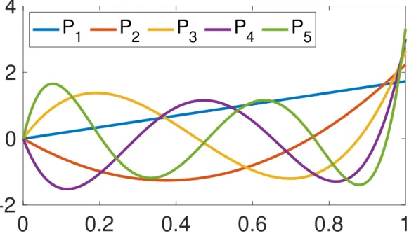
The orthonormal polynomial basis functions, generated using Gram-Schmidt orthogonalization,

are visualized in Fig. 3.3, and the coefficients that define the polynomials are shown in Table 3.1.

For example, P1(s) := 1.7321s, P2(s) :=−6.7082s+ 8.9943s2, etc.

0

0.2

0.4

0.6

0.8

1

-2

0

2

4

P

1

P

2

P

3

P

4

P

5

Figure 3.3: The orthonormal polynomial basis functions generated using Gram-Schmidt orthogonal-ization.

mechanics-based kinematics model based on the Cosserat Rod equations. Such pretraining allows us

to utilize a large amount of simulation data in order to prevent overfitting on the smaller amount of

sensed, real world data. Additionally, this allows the model to learn general characteristics of how

the concentric tube robot’s shapes are defined by the configuration from the simulation model, and

then to learn the ways in which the physical robot differs from simulation during fine-tuning.

We generated real world data by sampling uniformly at random configurations and pairing them

with the backbone they produced in the real world, which we sensed via shape from silhouette (see

Figs. 3.1 and 3.2). We then split our real world data into three sets. A training set of7,000data points, used to fine-tune the model, a validation set of 1,000 data points, used during training to evaluate convergence, and a test set of 1,000data points, which we left out for evaluating the performance of the network. We utilize a pointwise sum-of-squared-distances loss function and the

ADAM [28] optimizer during training. We utilize early exit of training at convergence as evaluated

by our validation set in order to prevent overfitting on the training set. If10,000epochs of training have passed without the model improving its performance as evaluated by the validation set, training

is stopped and the best version of the model found until that time is used.

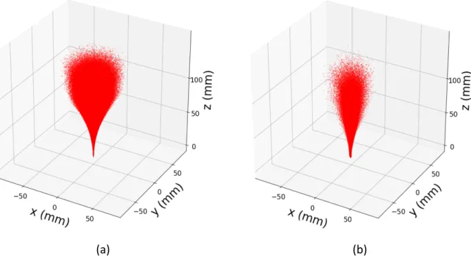
We demonstrate the motivation for the transfer learning approach in this application in Fig. 3.4,

in which we show a plot in the workspace of evenly spaced points along the backbone of every

configuration in our simulation training set in Fig. 3.4a and our real-world training set in Fig. 3.4b.

The simulation data set represents greater density throughout the workspace of the robot than is

(a)

(b)

Results

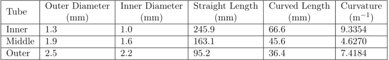
My collaborators and I conducted experiments to evaluate the performance of the method with

a 3-tube concentric tube robot. The specifications of the robot’s component tubes that were used in

the experiments are shown in Table 4.1.

4.1 Evaluation of Polynomial Basis Function

First, in order to evaluate how well the polynomial basis functions are able to approximate the

shape, we computed the optimal set of coefficients for the100,000 pre-training data points using ordinary least squares. We then evaluated how well the resulting shape representation approximated

the training data at 20 equally-spaced points along the backbone of the shape, as in the training

process. We then calculated the maximum L2 _{distance over the 20 points along the backbone of}

the robot between the polynomial representation and the ground truth for each of the 100,000

configurations. Over the 100,000configurations, the mean of the maximum L2 distance along the backbone was0.044±0.037mm. This demonstrates that the polynomial basis functions are capable of representing the shape of a concentric tube robot with accuracy well into the sub-millimeter range.

4.2 Evaluation of Varying Network Architectures

Next, we evaluate how well our model is able to learn the shape of real-world concentric tube

robot configurations across multiple network architectures. We train multiple networks with numbers

of hidden layers varying from 3to7 and numbers of nodes per hidden layer varying from15 to60. We also evaluate networks trained with simulated data alone (Sim), trained with real data alone

Table 4.1: Tube parameters for the 3-tube concentric tube robot.

Tube Outer Diameter (mm)

Inner Diameter (mm)

Straight Length (mm)

Curved Length (mm)

Curvature (m−1)

Inner 1.3 1.0 245.9 66.6 9.3354

Middle 1.9 1.6 163.1 45.6 4.6270

Table 4.2: Average Learned Model Accuracy Results (Mean ±Std in mm), Maximum Deviation Along Shaft

Model Architecture (width x depth)

Data Type 3x15 3x30 3x60 5x15 5x30 5x60 7x15 7x30 7x60

Sim 6.22±3.95 6.28±3.93 6.32±3.95 6.28±3.94 6.30±3.95 6.31±3.94 6.32±3.98 6.31±3.94 6.32±3.96 Real 3.93±2.50 3.66±2.40 4.08±2.41 4.38±2.43 3.81±2.35 4.11±2.46 3.95±2.34 3.65±2.31 4.68±2.58 Sim+Real 3.69±2.45 3.35±2.39 3.49±2.42 4.68±2.90 3.48±2.49 3.58±2.49 3.56±2.50 3.53±2.48 3.40±2.41

Table 4.3: Average Learned Model Accuracy Results (Mean ±Std in mm), Mean Squared Error Along Shaft

Model Architecture (width x depth)

Data Type 3x15 3x30 3x60 5x15 5x30 5x60 7x15 7x30 7x60

Sim 12.2±16.4 12.4±16.4 12.3±16.5 12.1±16.5 12.3±16.6 12.3±16.6 12.3±16.7 12.3±16.5 12.3±16.7 Real 4.73±6.29 3.50±5.13 5.03±6.61 4.44±4.89 3.49±4.72 4.06±5.21 3.96±4.81 3.54±4.64 4.96±5.08 Sim+Real 3.60±5.44 3.03±4.84 3.31±5.27 5.94±8.56 3.25±5.53 3.47±5.86 3.36±5.63 3.36±5.66 3.11±5.24

(Real), and pre-trained with simulated data and fine-tuned with real data (Sim+Real). We evaluate

each model’s error on the test set of1,000data points. For each configuration of our 3-tube robot a forward pass through each network is performed to determine the coefficients for the shape function.

We then evaluate that function and the ground truth from the vision system at 20evenly spaced points along the robot’s shaft. We evaluate the results using three different error metrics.

1. Maximum deviation along the robot’s shaft—the L2 distance of the point that deviates from

the ground truth the most. This error value presents us with a maximum deviation between

the predicted shape and the ground truth, a useful metric when considering safety related to

anatomical obstacle avoidance.

2. Mean squared error along the robot’s shaft—the squared L2 distance from the ground truth,

averaged along the robot’s shaft.

3. Sum of the deviations along the robot’s shaft—the L2 distance from the ground truth, summed

along the robot’s shaft.

I present the results of this analysis in Tables 4.2, 4.3, and 4.4. For each data type and architecture

I report the mean and standard deviation of the error (in mm) across all test data points. For each

Shaft

Model Architecture (width x depth)

Data Type 3x15 3x30 3x60 5x15 5x30 5x60 7x15 7x30 7x60

Sim 48.7±21.8 48.9±22.0 48.8±21.8 48.6±21.7 48.8±22.0 48.8±21.8 48.8±22.0 48.7±21.8 48.8±22.0 Real 31.2±13.7 25.8±10.9 33.2±12.0 30.1±11.5 25.8±10.6 28.4±10.7 28.6±11.3 26.8±10.7 31.8±11.5 Sim+Real 25.7±11.4 23.2±10.9 24.5±11.2 33.5±14.3 24.3±11.0 25.1±11.5 24.7±10.9 24.8±11.1 23.8±10.8

all architectures except 5x15, but to a lesser extent. This result aligns with the theory behind

transfer learning [9], which holds that pre-training on a large data set from a related domain and

then fine-tuning on a smaller data set from the exact domain of interest allows the model to learn

the general properties of the related domain first, and then to be refined on the nuance of the exact

domain. The best model for all three error metrics is trained on Sim+Real data, and has 3hidden layers of30 nodes each.

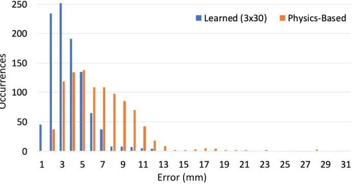
4.3 Accuracy Comparison to Physics-Based Model

Next, I compare the accuracy of the best model from the previous analysis to the physics-based

model presented in [7]. In Fig. 4.1 I plot a histogram of the errors across the1,000test configurations for the maximum deviation error metric.

Error (mm)

Oc

cu

rr

en

ce

s

Table 4.5: Error value statistics for the physics-based model and our learned model across the 1000

test configurations, Maximum Deviation Along Shaft.

Physics-Based (mm) Learned (mm)

Minimum 1.11 0.61

Maximum 46.68 30.18

Mean 6.32±3.95 3.35±2.39

Table 4.6: Error value statistics for the physics-based model and our learned model across the 1000

test configurations, Mean Squared Error Along Shaft.

Physics-Based (mm) Learned (mm)

Minimum 0.30 0.05

Maximum 246.62 82.58

Mean 12.32±16.60 3.03±4.84

In Tables 4.5, 4.6, and 4.7, I present further statistics for the maximum error values over the

1,000 test configurations for both the physics-based model and the learned model for the three error metrics. In the histogram in Fig. 4.1, it can be seen that the error distribution of the learned model

is shifted to the left compared with that of the physics-based model, indicating that the learned

model is more likely to produce lower error values than the physics-based model. Additionally, the

learned model produces lower minimum, maximum, and mean error values for all metrics.

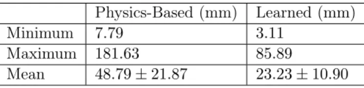
Table 4.7: Error value statistics for the physics-based model and our learned model across the 1000

test configurations, Sum of Deviations Along Shaft.

Physics-Based (mm) Learned (mm)

Minimum 7.79 3.11

Maximum 181.63 85.89

0

1

2

3

4

5

6

1 2 3 4 5 6 7 8 9 10 11 12 13 14 15 16 17 18 19 20

Av

g.

E

rr

or

(

m

m

)

Index Along Backbone

Learned (3x30)

Physics-Based

Figure 4.2: The L2 distance of points along the robot’s shaft between the ground truth and those computed by our learned model (blue) and between the ground truth and those computed by the physics-based model (red), plotted over the length of the robot’s shaft indexed from the first position at the base of the robot (where the error is 0 for both models), to the twentieth point at the robot’s tip. The error for both models is greatest at the tip of the robot. The values are averaged over the

1,000test data points.

In Fig. 4.2, I plot the error of our model and the physics-based model as a function of the position

along the robot’s backbone, averaged over the 1,000 test configurations. I note that for both the physics-based model and our learned model the error increases closer to the robot’s tip.

In Fig. 4.3 I show three shapes computed by our learned model compared to the ground truth

shapes. I plot in Fig. 4.3a the configuration whose error is closest to one standard deviation below

the average error (maximum deviation error metric), Fig. 4.3b shows the configuration whose error is

closest to the average error (maximum deviation error metric), and Fig. 4.3c shows the configuration

whose error is closest to one standard deviation above the average error (maximum error metric).

4.4 Speed Comparison to Physics-Based Mode

Both control and motion planning for concentric tube robots require many shape computations

to happen in a very short amount of time. This necessitates a shape model that is sufficiently fast to

compute. One advantage of using neural networks for our learned shape model is that computation

(a) (b) (c) Learned Ground Truth

Figure 4.3: I show three examples of the shape our learned model computes compared with the ground truth shape sensed in the same configuration. (a) I plot the shape whose error is closest to one standard deviation below the average error, (b) the shape whose error is closest to the average error, and (c) the shape whose error is closest to one standard deviation above the average error (using the maximum deviation along the robot’s shaft error metric).

shape computations) simultaneously, and it is almost as fast as computing a single pass. This process,

called batching, allows for many shape computations to happen very quickly in parallel, a property

that the physics-based shape model does not currently share.

In Fig. 4.4 I present the time required by each of the Sim+Real networks to perform shape

computations. I perform 100,000 shape computations for each, with batch sizes varying from 1

(i.e. no batching) to 100,000 (i.e. computing all shapes simultaneously). Included in the timing results are the time required to make the passes through the network as well as the time required to

Batch Size

Av

g.

T

im

e

pe

r S

ha

pe

C

om

pu

ta

tio

n

(ms

Figure 4.4: The average time taken to compute the shape of the concentric tube robot at a specified configuration, for20 evenly spaced points along its backbone. I present the average for each network topology (Sim+Real), for varying batch sizes. For comparison, the physics-based model averages 1.73ms per shape computation.

As can be seen, the models of less complexity (fewer hidden layers and fewer nodes per layer) are

faster. Additionally, increasing the batch size dramatically reduces the time per shape computed,

with the fastest (100,000 batch size) taking on average≈0.01ms per shape computation across all models. Without batching, the models range between0.27ms and 0.51ms per shape computation. These values represent a significant speed-up compared to the physics-based model which takes on

average1.73ms per shape computation. Without batching, the learned models are between3.39and

6.4times faster than the physics-based model, and with the largest batching, the learned models are ≈173times faster than the physics-based model.

While it is not as easy to take advantage of batching during traditional control of concentric

tube robots, due to the iterative nature of the required shape computations, during sampling-based

CHAPTER 5

Discussion and Conclusion

I presented a learned, neural network model that outputs an arc length parameterized space

curve. This allows us to take a data driven approach to modeling the shape of the concentric tube

robot and improve upon a physics-based model. This may allow for safer motion planning and

control of these devices in surgical settings that require avoiding anatomical obstacles, as a shape

that deviates less from the shape predicted in computation will be less likely to unintentionally

collide with the patient’s anatomy.

I note many areas of potential future investigation. Our model is only trained on cases where

the robot is operating in free space. There exist many surgical tasks that require minimal force to

be exerted by the robot on tissue that our method would be well suited for, such as using the robot

as an endoscope via a chip-tip camera, utilizing the robot to deliver energy-based ablation probes,

and utilizing the robot as a suction or irrigation catheter. However, many surgical tasks will require

non-trivial tissue interaction forces. In the future, my collaborators and I intend to train models

that account for the robot’s interaction with tissue both at its tip and along the shaft of the robot.

There are also many avenues to investigate additional machine learning techniques and

param-eterizations related to the method. For instance, we note the relatively minor improvement we

observed when combining simulated and real training data compared to using only real training data.

While in a minimally invasive surgical setting, any improvement to model accuracy is important,

we intend to further investigate ways to leverage the combination between real training data and

simulated training data to identify the role that simulated training data may play in model accuracy.

It may also be valuable to investigate the integration of learning with the physics-based concentric

of tubes or tube parameters.

We also intend to augment the learned model to account for other sources of uncertainty in

concentric tube robot shape modeling, including hysteresis. There also exist other choices of basis

functions. We chose orthonormal polynomials due to their fast evaluation, but we intend to investigate

other types of bases for our shape representation. These and other model parameter choices may

have implications on the types of shapes that it is able to predict well and the types that it predicts

less well. We consider a future characterization of this relationship to be important.

Further, we plan to integrate the learned model with a motion planner and evaluate its use in

automatic obstacle avoidance during tele-operation or automatic execution of surgical tasks.

Finally, we believe that this approach is not limited to concentric tube robots, but could be used

REFERENCES

[1] H. B. Gilbert, D. C. Rucker, and R. J. Webster III, “Concentric tube robots: The state of the art and future directions,” in Int. Symp. Robotics Research (ISRR), Dec. 2013.

[2] J. Burgner-Kahrs, D. C. Rucker, and H. Choset, “Continuum robots for medical applications: A survey,” IEEE Trans. Robotics, vol. 31, no. 6, pp. 1261–1280, 2015.

[3] L. G. Torres and R. Alterovitz, “Motion planning for concentric tube robots using mechanics-based models,” in Proc. IEEE/RSJ Int. Conf. Intelligent Robots and Systems (IROS), pp. 5153– 5159, Sept. 2011.

[4] L. G. Torres, A. Kuntz, H. B. Gilbert, P. J. Swaney, R. J. Hendrick, R. J. Webster III, and R. Alterovitz, “A motion planning approach to automatic obstacle avoidance during concentric tube robot teleoperation,” in Proc. IEEE Int. Conf. Robotics and Automation (ICRA), pp. 2361– 2367, May 2015.

[5] A. Kuntz, M. Fu, and R. Alterovitz, “Planning high-quality motions for concentric tube robots in point clouds via parallel sampling and optimization,” in Proc. IEEE/RSJ Int. Conf. Intelligent Robots and Systems (IROS), Nov 2019. to appear.

[6] S. M. LaValle, Planning Algorithms. Cambridge, U.K.: Cambridge University Press, 2006.

[7] D. C. Rucker,The mechanics of continuum robots: model-based sensing and control. PhD thesis, Vanderbilt University, 2011.

[8] G. Fagogenis, C. Bergeles, and P. E. Dupont, “Adaptive nonparametric kinematic modeling of concentric tube robots,” inIEEE/RSJ International Conference on Intelligent Robots and Systems (IROS), pp. 4324–4329, Oct. 2016.

[9] S. J. Pan and Q. Yang, “A survey on transfer learning,” IEEE Transactions on knowledge and data engineering, vol. 22, no. 10, pp. 1345–1359, 2009.

[10] A. Kuntz, A. Sethi, R. J. Webster, and R. Alterovitz, “Learning the complete shape of concentric tube robots,” IEEE Transactions on Medical Robotics and Bionics, 2020.

[11] A. Kuntz, A. Sethi, and R. Alterovitz, “Estimating the complete shape of concentric tube robots via learning,” inHamlyn Symposium on Medical Robotics, 2019.

[12] K. Leibrandt, C. Bergeles, and G.-Z. Yang, “Concentric tube robots: Rapid, stable path-planning and guidance for surgical use,” IEEE Robotics & Automation Magazine, vol. 24, no. 2, pp. 42–53, 2017.

Proc. SPIE Medical Imaging, vol. 7261, Mar. 2009.

[17] L. G. Torres, C. Baykal, and R. Alterovitz, “Interactive-rate motion planning for concentric tube robots,” in Proc. IEEE Int. Conf. Robotics and Automation (ICRA), pp. 1915–1921, May 2014.

[18] R. Xu, A. Yurkewich, and R. V. Patel, “Shape sensing for torsionally compliant concentric-tube robots,” inOptical Fibers and Sensors for Medical Diagnostics and Treatment Applications XVI, vol. 9702, p. 97020V, International Society for Optics and Photonics, 2016.

[19] M. B. Rubin,Cosserat Theories: Shells, Rods and Points. Springer Science & Business Media, 2000.

[20] S. S. Antman,Nonlinear Problems of Elasticity. Springer, 1995.

[21] H. B. Gilbert, D. C. Rucker, and R. J. Webster III, “Concentric tube robots: The state of the art and future directions,” in Robotics Research, pp. 253–269, Springer, 2016.

[22] W. Xu, J. Chen, H. Y. Lau, and H. Ren, “Data-driven methods towards learning the highly nonlinear inverse kinematics of tendon-driven surgical manipulators,” The International Journal of Medical Robotics and Computer Assisted Surgery, vol. 13, no. 3, p. e1774, 2017.

[23] M. Giorelli, F. Renda, M. Calisti, A. Arienti, G. Ferri, and C. Laschi, “Neural network and jacobian method for solving the inverse statics of a cable-driven soft arm with nonconstant curvature,” IEEE Transactions on Robotics, vol. 31, no. 4, pp. 823–834, 2015.

[24] A. Melingui, R. Merzouki, J. B. Mbede, C. Escande, and N. Benoudjit, “Neural networks based approach for inverse kinematic modeling of a compact bionic handling assistant trunk,” in 2014 IEEE 23rd International Symposium on Industrial Electronics (ISIE), pp. 1239–1244, IEEE, 2014.

[25] C. Bergeles, F. Y. Lin, and G. Z. Yang, “Concentric tube robot kinematics using neural networks,” inHamlyn Symposium on Medical Robotics, pp. 1–2, June 2015.

[26] R. Grassmann, V. Modes, and J. Burgner-Kahrs, “Learning the forward and inverse kinematics of a 6-dof concentric tube continuum robot in se(3),” inIEEE/RSJ International Conference on Intelligent Robots and Systems (IROS), (Madrid, Spain), pp. 5125–5132, Oct. 2018.

[27] S. Baker and T. Kanade, “Shape-from-silhouette across time part I: Theory and algorithms,”

International Journal of Computer Vision, vol. 62, no. 3, pp. 221–247, 2005.