Bayesian Model Based Approaches In The Analysis Of
Chromatin Structure And Motif Discovery
by Riten Mitra
A dissertation submitted to the faculty of the University of North Carolina at Chapel Hill in partial fulfillment of the requirements for the degree of Doctor of Philosophy in the Department of Biostatistics.
Chapel Hill 2010
Approved by:
Dr P.K.Sen, Advisor
Dr Mayetri Gupta, Committee Member
Dr Joseph Ibrahim, Committee Member
Dr Fred Wright, Committee Member
ABSTRACT
RITEN MITRA: Bayesian Model Based Approaches In The Analysis Of Chromatin Structure And Motif Discovery.
(Under the direction of Dr P.K.Sen.)
Contents
List of Tables vi
1 Introduction 1
2 Literature Review 6
2.1 Introduction . . . 6
2.2 Algorithms for motif discovery . . . 7
2.2.1 Position Weight Matrix models . . . 9
2.2.2 Inference in Position Weight Matrix Models . . . 10
2.2.3 Extensions . . . 11
2.2.4 Dictionary models . . . 13
2.2.5 Relaxing the Product Multinomial assumption . . . 16
2.3 Using auxiliary information in motif discovery . . . 18
2.3.1 Evolutionary conservation . . . 18
2.3.2 Gene expression . . . 20
2.4 Statistical modeling of chromatin structure . . . 22
2.4.1 The biology of Nucleosomes . . . 22
2.4.2 Nucleosome prediction algorithms . . . 23
2.4.3 Relationship with sequence features . . . 26
2.4.4 Mapping positions and its connection with motif search . . . 30
2.5 Statistical inference in hidden Markov models . . . 31
2.5.3 Alternative Estimation Methods . . . 36
2.5.4 L mixing processes . . . 38
2.5.5 Conclusions . . . 39
3 Determining chromatin features using continuous time hidden Markov models 40 3.1 Introduction . . . 40
3.1.1 Genomic assays for nucleosome position detection . . . 41
3.1.2 Computational approaches for nucleosome detection . . . 42
3.2 Model framework . . . 44
3.2.1 Data structure . . . 45
3.2.2 Continuous index hidden Markov process . . . 45
3.2.3 Adding covariate effects to the model . . . 47
3.2.4 Identifiability . . . 49
3.3 Model-fitting and Estimation procedure . . . 50
3.3.1 Prior elicitation and sensitivity analysis . . . 52
3.3.2 The MCMC sampling algorithm . . . 53
3.4 Details of sampling procedure . . . 55
3.4.1 Step I–Sampling the transition parameters . . . 57
3.4.2 Step II : Sampling of emission parameters . . . 58
3.5 Application to yeast nucleosome array data . . . 60
3.5.1 Model-fitting using three models . . . 61
3.5.2 Comparison with known NFR regions from UCSC genome browser . 64 3.6 Simulation studies . . . 64
3.6.1 Consistency of model parameter estimation . . . 65
3.6.2 Cross comparison under different models . . . 66
3.6.3 Importance of the continuous index model . . . 68
3.7 Discussion . . . 68
4 A joint model approach to motif finding, using nucleosomal information 74 4.1 Introduction . . . 74
4.2.1 Data Structure and Assumptions . . . 76
4.2.2 Observed data and latent variables. . . 77
4.2.3 Model formulation. . . 77
4.3 Estimation Procedure-The Setup . . . 79
4.4 Estimation Procedure . . . 79
4.4.1 Forward Algorithm I . . . 80
4.4.2 Forward algorithm II . . . 81
4.4.3 Forward algorithm III to be used for joint sampling . . . 82
4.5 Sampling scheme and Conditional distributions . . . 83
4.6 Simulations . . . 87
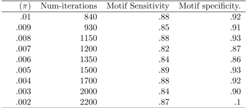
4.6.1 Parameter Settings and inference methods for the simulation studies 88 4.6.2 Checking convergence pattern with π . . . 90
4.6.3 Initial values for the MCMC chain . . . 91
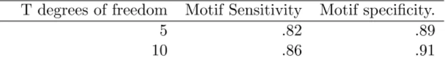
4.6.4 Changing distributional assumptions . . . 93
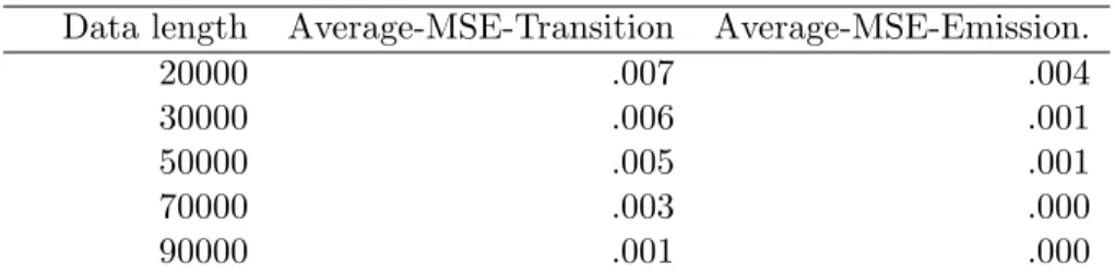
4.6.5 Consistency . . . 93
4.6.6 Varying Beta and Motif occurrence Probability simultaneously . . . 94
4.6.7 Motif Categories 0 and A . . . 95
4.6.8 Motif Category B . . . 96
4.6.9 Mis-specifying the motif width . . . 97
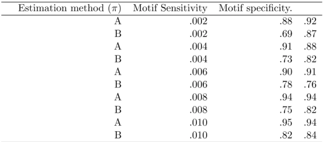
4.6.10 Two Step approach and its comparison with the joint model . . . 98
4.7 Identifiability . . . 98
4.8 Structure of the hidden Markov model . . . 101
4.9 Results . . . 101
4.9.1 Applications on the yeast genome data set . . . 101
4.9.2 Comparison with the denovo motif discovery and the two-step method103 4.10 Conclusions . . . 104
5 Asymptotic results for continuous time hidden Markov models 106 5.1 Introduction . . . 106
5.2 Asymptotic inference for parameter estimates, score and information in
con-tinuous time HMMs . . . 108
5.2.1 The main results . . . 108
5.3 Consistency . . . 109
5.3.1 Identifiability . . . 111
5.3.2 Identifiabilty and Asymptotics of log likelihood gives us consistency 114 5.4 Asymptotic Normality of the score function . . . 114
5.5 Contiguity . . . 117
5.6 Posterior Convergence . . . 121
5.6.1 The proof of asymptotic convergence of posterior density under a continuous prior . . . 122
5.6.2 Consequences of posterior consistency and convergence on Bayesian inference in nucleosome positioning models . . . 126
5.7 Conclusions . . . 129
6 Conclusion and Future directions 131
List of Tables
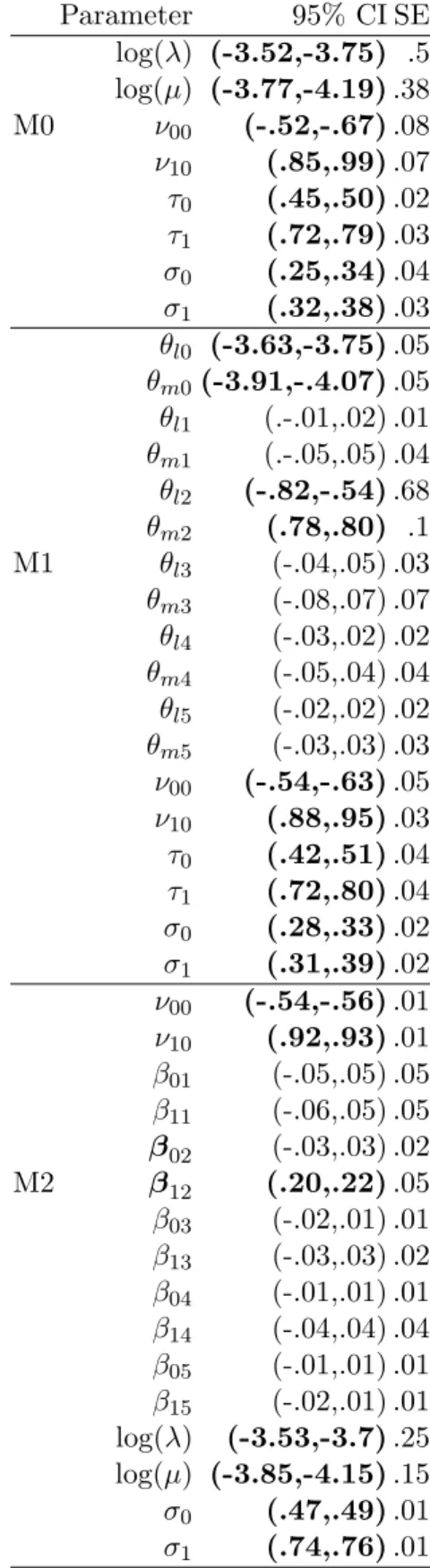
3.1 Panel 1: 95% Credible Intervals (CI) for parameter estimates for models M0 (base), M1 (transition), and M2 (emission). The indicesl (or 0) and m (or 1) indicate the nucleosomal and NFR states; for instance, the termθl0 refers
to the intercept term for the nucleosomal state in the transition model M1, ν10refers to the intercept term for the NFR state in the emission model M2.
The CIs for parameters significant at a 95% level are given in bold fonts. Panel 2: Principal component weights of the significant covariate from the
emission and transition models. . . 71
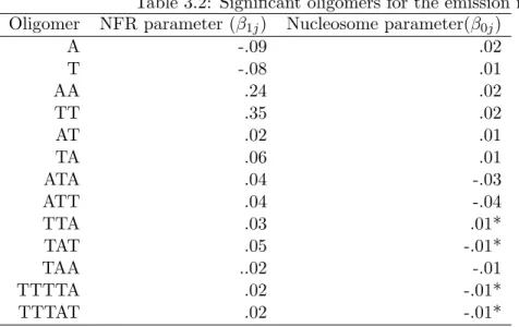
3.2 Significant oligomers for the emission model . . . 72
3.3 Significant oligomers for the transition model . . . 72
3.4 Simulation study:Proportion of datasets classified under the true model by the BIC criterion . . . 73
3.5 Tabulation of (a) correct state classification percentage ( Match”) and (b) Bayesian Information Criterion for model M3 under the three estimation models. . . 73
3.6 Simulation study to compare the performance of discrete-index and continuous-index HMMs under two gap scenarios . . . 73
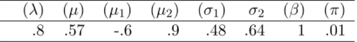
4.1 Parameter values . . . 88
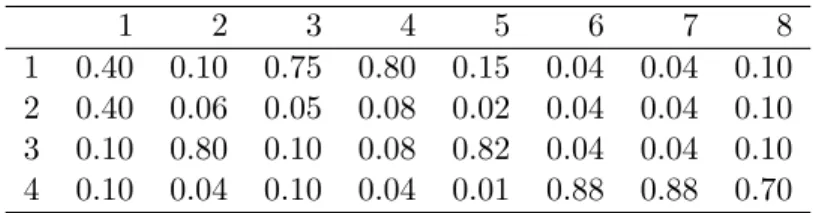
4.2 Motif matrix . . . 89
4.3 Convergence pattern . . . 90
4.4 Robustness . . . 93
4.5 Consistency of Parameter Estimates . . . 94
4.6 Comparison with the two step approach . . . 99
4.7 Parameter values . . . 102
4.8 Estimated Motif Matrix . . . 102
Chapter 1
Introduction
Research in computational biology over the past few decades has consistently
supplemented and strengthened the field of genomics. It plays as much important a role in paving the the path to discoveries of great consequence, as the laboratory methods. The field has arisen out of a demand to address the new questions posed by the size and nature of the genomic data that has been in proliferation. These data arising out of new technological setup, has features and characteristics of its own. This, in turn, has led to framing innovative statistical methodologies and algorithms. Most of these algorithms are centered around a Bayesian paradigm, mostly in the field of motif discovery.
trying to incorporate secondary information in the form of presence or absence
nucleosomal structures. The secondary information has come up in . But our methods that we have implemented are just not based on merging of two data sources in coming up with more information . It goes beyond that in the sense that it implements the merger efficiently so that propagation biases from one prediction to another gets
minimized. This issue has led us to come up with a suitable statistical model that jointly samples nucleosomes and motifs.
This modeling framework gives a biologically plausible structure to the data and forms one part of the picture. The other part comes from the set of issues originating from type of data that we are dealing with. The FAIRE technology that outputs the genome wide intensities has missing information inform of non contiguous probes. This must be dealt with first before we could possibly extend our nucleosome prediction models into a joint model. The first chapter is concerned with implementation and evaluation of such a model. We have been able to incorporate sequence features directly into the link function of a model to see if sequence features has an influence on the length of nucleosome and the propensity of nucleosome occurrence ( measured by intensity data) Having satisfied ourselves that this framework produces remarkably favourable results on comparison with known data bases, and provides a significant improvement over the currently used HMM methods on modelling accurately the location features. we have been encouraged to build up on it and venture into the joint model described above. The joint model instead of one has two layer of hidden states, one for the nucleosome and one for the data structure. The data sources come in the form of nucleosomal intensity data and sequence data, obtained from Chip-Chip experiments and microarrays. The recursive forward algorithm that we implemented for the first chapter gets extended into a modified algorithm with two running indices for the two hidden states.
The inferences both from the joint model and the nucleosomal model ( which consists of a single layer of hidden states) is aided by MCMC sampling from the posterior. The
non informative background on the parameters to be inferred, and make our inferences solely based on the data alone. The flat prior assumption essentially enables us to analyze the likelihood function and its properties through MCMC sampling techniques. So our inference on Maximum Likelihood Estimation of a a continuous time hidden markov model gets directly translated into making inferences on the posterior mode of the Bayesian model. By our conclusions in the third chapter, we have shown that the this mode is a consistent estimator. That is , under large sample size conditions the posterior mode is very close to the true parameter values. This is a very important and immensely relevant result considering the size of the genomic data that wee handle. In our
application the sequence size runs in arange of 340000-500000 base pairs. Taking the mode of our posterior samples from MCMC would give us a very accurate prediction of the parametrs governing the underlying hidden markov process, and we would be able to predict the DNA structural positions to a very high degree of accuracy. This result has scopes beyobnd the applications that we have considered in the first two chapters and can find useful application in numerous classification and optimization problems in genomics which are based on likelihood approach .
We have taken the techniques of analyzing the HMM likelihood one step further and proved the asymptotic normality of the score function and the maximum likelihood estimates. This enabled us in building asymptotic confidence intervals of the sampled posterior mode of the parameters. By examining the position of the null with respect to the upper and lower bound of the interval we assessed the significance of the parameters. The fascinating thing about this result is that we no longer have to depend on the simulation sample sizes in order to get an estimate of the interval length, but we could directly obtain it from a single round of computations from the complete data likelihood. The MLE results and consistency are based on simple assumptions on the boundedness of transition parameters. By the biological constraints on the length of the nucleosome free regions and the nucleosomes, these conditions are trivially satisfied.
This methodology gives us a statistically rigorous estimate of the distance of our
estimates from the null distribution However in some cases we need to assess the power of our test statistics under suitable alternatives For example we need to know if for
nucleosomal lengths. Or in the case of yhe joint model, if a weak link joining the motif strength and signal is existent. Sometimes we are dealing with weakly pronounced motif signals that are not very different from the background and hence is difficult to
distinguish or pick up. Here the decreasing genomic distance on the phylogenetic tree between related species, or the link value tending towards 0 or the weak motif signals, denote a sequence of alternatives tending towards the null. and testing procedures would necessitate deriving the distribution of power statistics under these conditions. This ahs been facilitated by the property of contiguity which we have been able to derive for the continuous time HMM. The contiguity property relied on asymptotic noramlity of the log likelihood and the asymptotic similarity of the observed and expected Fisher Information. The third chapter thus provides a repertoire of statistical tools to supplement our
inferences in the first and the second. The document is organized as follows. The first chapter introduces the continuous hidden markov model and extends it to include sequence features. By implementing the model on a well known data set, we have been able get new insights into the relationships between nucleosomes and DNA
characteristics. The second chapter of our document describes a nucleosome-motif model and quantifies the link between gene signal and motif strength. The third chapter deals with asymptotics of the models described above and provides the setup for testing hypothesis under biologically plausible local alternatives. The last chapter gives an overview of the body of work and points to the future directions in this area.
certain sophisticated theoretical tools in the proof of maximum likelihood
estimation–which have been a recurrent theme in work done in this area. Within the same section, I have provided a short description of our proposed method, which attempt to extend the known results of discrete HMM to its continuous time version.
Chapter 3 deals with the first paper of our proposal. These sections give the motivation of our proposed method, describe in detail the biological background and data
structure,provide an explanation of our estimation techniques, and show clearly the potential of our newly developed methodology to contribute significantly to current research.
The next major division, Chapter 4, constitutes the content of our second paper. It talks about a joint model that uniquely combines nucleosome finding, and motif search into a single Bayesian framework.
Chapter 5 talks about the asymptotic results and the contiguity arguments thereof. The concluding chapter 6 deals with future directions of research.
Chapter 2
Literature Review
2.1
Introduction
The DNA sequence can be viewed as a series of letters taken from the set ( A C G T), which correspond to the nucleotides Adenosine, Thymine, Cytosine and Guanin
respectively. In reality, we do not have a single sequence, but a double helical structure, where one strand has the ’complementary’ base, relative to another. Due to the chemical affinity formed from their structure, these nucleotide pairs form matching pairs. For example, if we take a subsection of one DNA strand and observe the sequence ACGT we can readily infer that the other strand has TGCA in the same positions. This
complementarity allows us to focus our attention on a single DNA strand.
Since its discovery as the key constituent of cellular life in living organisms, attempts have been made to unearth the information contained in the genome. Advances in technology in the last two decades have made it possible to (a) make a map of the DNA sequence pattern and (b) reveal the physical structure of DNA. The DNA sequence, when considered alone, does not adhere to a regular deterministic pattern. Today,however, we know that there are subsequences in the DNA called genes, which are the key
constituents in initiating the bio-chemical processes that lead to the formation of proteins in our cell, thus acting as the building block for all life processes in an organism.
Transcription is the first step in the process. It is onset when the enzyme RNA
the DNA sequence to be copied into mRNA. The information is then transferred from mRNA by the process of translation to form proteins. A special group of proteins, called the ’transcription factors’ interacts with RNAp and regulate gene expression. They do so by attaching themselves to certain regions in the upstream section of a gene. The binding of transcription factors is a chemical process that depends on the binding energy of the interacting molecules,(the biology of which is not fully understood till date) and the chromatin structure of the region. Knowledge of the location of these binding sites would serve as a very useful guide in locating the functionally important regions of the genome, and hence ranks as one of the most important quests facing the field of bioinformatics today.
Experimental detection of the transcription factor binding sites remain an infeasible task. Hence, much of the work done in this direction, relies on statistical and numerical
algorithms that exploit the quantitative differences in the base composition of the binding sites and the rest of the sequence. The binding sites are typically 8-20 base pairs long. One important property of these sites is that the sequence structure is more or less conserved across all binding sites corresponding to a particular transcription factor. Mismatches or some random deviations from a fixed pattern are, however, tolerated. The underlying fixed pattern is called a ’motif’.
Motifs are, thus, defined to be short repetitive ( with some fuzzy mismatches )
subsequences of unknown length within a DNA sequence. So now, the biological problem of finding the transcription factor binding sites translates to the computational and statistical problem of locating motifs in a sequence. It is expected that probabilistic models will have a big role to play in the motif search algorithms, since the patterns are repetitive with a degree of fuzziness or random error. The following section gives us an overview of the motif discovery models and methodologies.
2.2
Algorithms for motif discovery
where k is the motif length. Each column corresponded to a position in the binding site, and the frequencies in each column denoted the frequencies of occurences of different base pairs in that particular position. Initially all k length words ( contagious subsequences) were chosen from one sequence . These words were equivalent to several 4 x k matrices where the first row is 1. In other words these initial choice of motifs were free of any random error components. Next, each of these matrices were compared to all k-length words from the next sequence. The comparison was quantitatively done using the Kullback- Liebler information score
IKL = X
i X
j
fijlog fij f0j
where i ranged over the positions and j is the index of the base pair. For each matrix, the highest score was retained, and the k-word that gave rise to the score was added as a row in the matrix. The matrix was then normalized to the relative frequency scale. This was done progressively over all sequences and the highest scoring matrices were retained. Although computationally feasible, the above method lacked in a rigorous statistical framework that would allow us to test the significance of the motifs obtained. The scoring criterion, though having the intuitive appeal, was also chosen arbitrarily. This motivated researchers in the early 90s to come up with more rigorous stochastic models, that aimed in determining simultaneously the unknown matrix (the motif pattern) and the sites of their occurrence. Attempts to construct such a model was first taken by Lawrence and Reilly(1993). In their formulation, the sequences were allowed to have only one motif site . This was a restrictive assumption. Also, the model was based on the fact that there would be only one motif pattern prevalent in the entire set of sequences-not a valid assumption.
2.2.1 Position Weight Matrix models
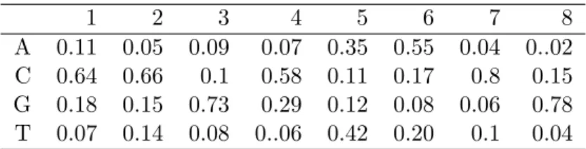
We have N different sequences withSi of length Li. For k different motif types, the k Position Weight matrices are denoted as Θ = Θ1, ...Θd. Each Θk= (θk1, θk2....θwk) wherewk is the width of the kth motif type and θki = (θki1, θki2θki3, θki4) denotes the
probabilities of the 4 bases to occur in theith binding position of motif type k. The corresponding probabilities for the distribution of sequences under the background ( i.e in places not occupied by motifs) is denoted by θ0 = (θ01, θ02θ03, θ04).
The start position of the motif sites is indicated by the indicator variable
A= ((Aijk)) = 1 iff position j in sequence i, is the start position of the motif type k. Ak denotes the indicator variable for the start position of the motif type k, spanning all sequences. LetSAki denote the set of letters occuring in position i of every instance of motif type k. If C(S) denotes the set of frequencies of all letters in a set S, then (C(SAk1 ), ...C(Swk
Ak)) follows Product multinomialM N(θk1, ...θkwk) i.e the ith
position in the motif type k, has column frequencies that follow a multinomial model with parametersθki.
Using the notationuv =Qpi=1uvii for vectors u and v inRp the likelihood conditioned on the indicator matrix A is
P(S|Θ, A, θ0) =θC(S
Ac) 0 K Y k=1 wk Y i=1
θC(S Ak i )
ki (2.2.1)
The prior assumed onθ0 is Dirichlet(β0) whereβ0= (β01...β0K) and the corresponding Dirichlet prior is PD(B) for Θk whereB = (βk1, ....βkwk) is a 4 by wk matrix. π denotes the probability that any position is a motif start site, i.eπ =P(A(ijk) = 1). The prior assumed onπ is Beta(α, β) The posterior conditional probability of the data can now be written as
P(Θ, A, θ0|S) =θC(S
Ac)+β
0 0 K Y k=1 wk Y i=1
θC(S Ak i )+βki
ki , (2.2.2)
2.2.2 Inference in Position Weight Matrix Models
Since the full conditionals are easily available, straight forward Gibbs sampling of the parameters is one possible approach. However for computational efficiency, Θ andπ can be integrated out and sampling could be done directly from the posterior distribution P(A/S). The sampling of A would be then done using a Gibbs method, i.e. conditioned on the presence or absence of motif sites elsewhere in the set of sequences sequence, the probability of having a motif of type k, start at a particular position, is calculated. The position is then assigned to a possible motif start position with the calculated probability. Based on an approximation, Liu et al Liu et al. (1995) computed the following predictive formula
P(A(ijk) = 1/S) P(A(ijk) = 0/S) =
π 1−π
wk Y i=1
ˆ θkl
ˆ θ0
C(Si,j+1,k) where ˆθkl and ˆθ0 are the estimated posterior means.
The above formula is intuitively appealing, since it shows directly the influence of the nucleotide counts of the motif models ( the matrix column counts updated by the
Bayesian parameters go into the posterior mean estimates). However the Gibbs approach becomes ’sticky’, when the motif sites are abundant. (This is because we shall not be able to sample till after w positions of a selected motif site.)
One alternative to this would be to use a Data Augmentation technique. Under this approach we do not integrate outθand π but conditioned on these parameters draw directly from the joint distribution of A. However, the conditional distribution of A does not have a closed form. To get rid of this problem, the algorithm of forward summation and backward sampling is implemented. This algorithm plays a key role in computational genomics and is widely used for models with unobserved hidden states.
background.
F(j, k) = X k≥0
F(j−w, l)θC(Sj−w:j)
k , k≥1 (2.2.3)
F(j,0) = X k≥0
F(j−w, l)θCb(Sj−w:j) (2.2.4) Backward sampling is then implemented to sample motif occurring sites from the end of the sequence. The rationale behind the backward sampling procedure is that the joint distribution of P(A|S) can be written as the product of conditional distributions.
We initiate the backward sampling by first selecting the last position of the sequence as a motif ending site of type k with probability
F(N, k) P
l6=kF(N, l)
If the position is selected as a motif of type k, we move back wsteps and sample at the N-w position.Else, we sample from the position N-1 with probability F(N-1, k). Generally for any position j, the probability of sampling a motif of type k is given as
F(j, k) P
l6=kF(j, l)
We continue the above chain of conditional sampling till we reach the beginning of the sequence. The beauty of the backward sampling is that the Markovian property makes the backward sampling probabilities only dependent on the forward probabilities, and not on the configuration of the previously sampled motifs.
2.2.3 Extensions
needed to be formulated for complex eukaryotes(e.g, humans, mouse) . This is because in such organisms, some potential problems can arise in the form of weak motif signals, sparseness of signals, ( the binding site might be 2000 base pair away from gene), and the tendency of motifs to occur in clusters.
In order to accommodate these features, a more complete Bayesian model was proposed that incorporated the distance between the motifs(λ), a correlation transition matrix reflecting the probability of transition between adjacent motifs -(τ ), and a variable list of putative motifs D= (D1, D2, ...Dp).
D0 denotes the background model.
The length,d, between the motifs is assumed to follow a geometric distribution with parameterλtruncated at w.
Let u denote a p-vector of binary random variables whereuj = 1 iff Dj is a part of the module. Thus number of non-zero entries in the vector u denote the number of motif types currently included in the model.
The prior distributions are as follows:
P(uj = 1) =π (2.2.5)
λ≈Beta(a, b) (2.2.6) Di =
k Y j=1
Dirichlet(βij) (2.2.7)
D0 ≈Dirichlet(β0) (2.2.8)
Theith row ofτ followsDirichlet(αi). The multinomial parameters have closed form conditional distributions, as previously. The indicator matrix of motif positions, A, could be sampled through the data augmentation technique by first recursively computing the forward likelihood and then implementing backward sampling. The forward algorithm and backward sampling procedure needs to be adapted to the extended parameter settings.
posterior probability is given as
P(u/A, T, S) =π|u|(1−π)p−|u| Z
P(S/A, T, Du)P(Du/u)d(Du)
Evolutionary Monte Carlo is then applied to sample u. A set of temperatures (t1...t) is
chosen for eachui . Now we define
φ(ui) =exp(log(P(u/A, T, S)/ti)
A new configuration is now selected by the following steps:
1. Mutation: A new configurationvk is chosen by randomly selecting uk and changing. uk is then replaced byvk with the probabilitymin(φφ((vkuk)),1)
2. Crossover: Two configurationsuk and uj are randomly selected and new unitsvj andvk are formed by a random exchange of their segments.
The two new units then replace the old ones with probability
min(φ(vk)φ(vj) φ(uk)φ(uj)
,1).
Alternative models for motif discovery were being suggested since early 2000, that employed the concept of segmentation of the sequence data. Recursive formulae for computation of likelihood formed the basis of inference in such models. Below,we present a short overview of one such category of models.
2.2.4 Dictionary models
ρ= [ρM1, ...ρMD] . H is the index for all possible segmentation of the sequence into
words. (H1, ...Hk) represents the possible partition of the sequence into k words.
Let N(H) denote the number of words in H,NM j(H) be the number of occurences of type Mj in the partition. The full likelihood of the data can be written as
P(S|ρ) =X H
Nh Y i=1
ρ(SHi) =X H
d Y j=1
[ρ(Mj)]NM j(H)
The likelihood does not have a closed form, but its computation can be made feasible by using the forward recursive formula below. LetFi denote the likelihood till position i. Then
Fi = w X j=1
ρ(Si−j:i)Fi−j
where w is the length of the longest word.
The maximum likelihood estimate of the parameters can be obtained through a Newton-Raphson algorithm. Alternatively, expectation maximization(EM) or Gibbs sampling can be used. The iterative procedure of estimation, introduced by Bussmeker et al,was to start off with an initial dictionary of only 4 single letter words (A, C, G,T) . At each stage of the dictionary, the maximum likelihood estimate of the word frequencies were computed. Based on these estimated probabilities, it was observed whether random concatenation of words were more probable than expected under the current model. These words were then added to the dictionary.
The above algorithm had two major drawbacks. One was that the algorithm would have the longer words consist of overrepresented segments, though that might not be true. The other was the fact that it overlooked the stochastic nature of motifs. An improved version of the above was presented in the paper by Keles et al(2003) [Keles et al. (2003)], where a probabilistic model was introduced to model the lengths of the first and last segments. A substantial improvement to the dictionary model was done in Gupta and Liu(2003) Gupta and Liu (2003) where the concept of a stochastic dictionary was first introduced. A stochastic dictionary consisting of D words is equivalent to D Position Weight
w is represented as (θ1, ...θwk). The occurrences of letters in motif sites corresponding to the same motif thus follow a product multinomial model. As in the notation defined in the earlier section,Aik represents the indicator of the motif type k beginning at position i. LetC = [Cq+1, ....CD] represent the count matrices corresponding to the probability matrices. The complete data likelihood is
L(N, C, A|ΘD, ρ) = D Y l=1
ρl D Y k=5
wk Y j=1
w Y i=1
θcijkijk
A Dirichlet distribution is assumed for
ρ≈Dirichlet(β0)
A corresponding Dirichlet prior PD(B)is assumed for Θk= [θ1k, ....θwkk] where
B=(β1, β2...βk) is a 4 x wk matrix, with each βj = (β1j, ..β4j) The posterior distribution of Θk is Product Dirichlet PD(B+Ck) i,e the column counts of thekth word are updated by the Beta prior coefficients.The posterior distribution ofρ is Dirichlet (N +β0). The
complete likelihood till theith position, L
i(Θ) is computed from a recursive formula identical to the Bussemaker’s model given above. Motif start sites are then conditionally sampled with the probability:
P(Aik = 1|Ai+wk,Θ) =
P(Si:i+wk−1,Θ, ρ)Li−1(Θ)
Li−1(Θ)
Next, the stochastic matrix parameters andρ is sampled from their conditional distributions, as given above.
The start sites and the motif parameters are sampled in this way till convergence. Then the number of words in the dictionary is incremented by 1 ( D=D+1) and the algorithm starts from step 1.
A particular motif alignment is scored by the MAP criterion ( Maximum A posteriori Probability). For a particular motif pattern A, the MAP is given by
P(A∗ |M1)
whereM0 denotes the model that the entire sequence is generated from background,
whileM1 is the model that incorporates motifs. P(A∗ |M1) is the maximum of the
posterior density of A.θis integrated out in order to calculate the numerator and denominator. The MAP score was tracked along with the steps of the algorithm.
2.2.5 Relaxing the Product Multinomial assumption
The product multinomial likelihood obtained in the position weight matrix models was derived from the assumption that the nucleotide occurrences at motif positions were independent.
This constraint was first relaxed in Zhou and Liu(2003) Zhou and Liu (2004) . The motif binding positions were allowed to be correlated with each other, but only pairwise
correlations were permitted. That is, a given position could be correlated with only one other position in the binding site.
The total model space, H is huge and containsHm, the space of models having m correlations. A prior was put on the model spaces so as to penalize the models with larger number of correlations. Also, all models having the same number of correlations were assigned equal weight. That is
P(H1) =P(H2)
ifH1 and H2 belong toHm
P(H1)
P(H2)
=Choose(w−2m,2)
i.e models that have larger correlations are given a weight inverse to the number of ways of inducing the additional correlations.
The prior probability for anyH ∈Hm is calculated as proportional to 2 m
(w−2m)!w!
The motif occurence probability is given asρ. ρ is assigned a Beta (a, b) prior. The usual Dirichlet priors are imposed on the motif and background parameters.
The joint distribution of the data and the unknown parameters can be written as
Sampling is done from the above distribution in the following steps.
1. Conditional on all other parameters, A is sampled through a Gibbs procedure.
2. ρ is sampled from its posterior distribution, Beta(a+|A|, L− |A|+b) 3. Motif parameters are sampled from their conditional distributions which are
Dirichlet.
4. Updating of H directly is a problem, since the dimension of the motif parameters change with the cardinality of H.
So the motif parameters andρ are integrated out from the joint posterior to give P(S, A|H).P(H|S, A) is proportional to P(SA|H)P(H).
H is now updated by a Metropolis-Hastings step. The new candidateH∗ is obtained in the following two ways:
Addition: A pair of positions is randomly selected from (w−2m) positions of the motif and added to H.
Deletion: A pair of positions is selected from the m correlated pairs and removed. We accept the new H∗ with the probability min( 1, r) where r is the ratio
P(H∗|S, A)T(H/H∗) P(H|SA)T(H∗|H)
and T is the proposal density. A phase shifting step is implemented once in every 20 iterations of the algorithm to escape local modes.
Alongside the product multinomial hypothesis, we usually assume that the conservation is uniform over all regions in a motif. Again this is not biologically true. In reality, transcription factors act over certain segments of DNA bases at a time. A fragmentation model was proposed in Liu and Lawrence that allowed for a prior to be set up on the motif positions,reflecting the importance of each motif position. Kechris et al Kechris et al. (2004) used a prior distribution ( normal or double exponential) that penalized deviations ( absolute or squared)from the conservation profile. The parameters were updated using EM algorithm.
The methodologies discussed above were de novo, in the sense that they did not use any external information for finding motif sites. These methods suffer from the disadvantage of poor predictive ability and a high false positive rate. Recently, with the remarkable improvement of genome output technology, there has been a proliferation of genomic data that has motivated researchers to take advantage of external information and incorporate them in motif search. The most important sources of these external information arise in the form of
1. Evolutionary data. Genomic data for comparing different species are now available to us. The conservation pattern in the binding sites are directly dependent on the inter-species evolutionary distance.
2. Gene expression
3. Data on the underlying chromatin structure.
2.3
Using auxiliary information in motif discovery
2.3.1 Evolutionary conservation
When multiple sequence information is available it has been seen that multiply aligning sequences and using regions having a high sequence similarity increases the specificity of motif search. Wasserman et al Wasserman et al. (2000) generalized the species
transcription factors are confined to the 19 percent of human sequences that are most conserved in the orthologous rodent sequences.
Based on the knowledge that regulatory regions are more conserved between human and mouse genomes than the background, Liu and Liu Liu et al. (2004) developed a method called Compare-Prospecter that extends Gibbs sampling by biasing the search in regions conserved across species. Recently, based on the interactions arising from clusters of TFBSs with known binding patterns, a variety of computational methods have been created for the discrimination of CRMs.
It is often the case that no prior information exists on binding patterns of any relevant transcription factors for sets of genes identified in large-scale expression studies. One approach is a method for identification of modules using known motifs, but it includes a preliminary step of motif identification using either a Gibbs sampling algorithm or an algorithm based on overrepresented oligonucleotide sequences One other approach uses suffix-trees and word consensus rather than a statistical model to locate ordered collections of motifs Marsan and Sagot (2000). In this method, sites of each motif type are assumed to occur exactly once in each module. An expectation-maximization algorithm based on a discriminant model with multiple iterative optimization steps has also been described Segal and Sharan (2005). Although these approaches are promising, computational identification of a TFBSs without prior knowledge of binding patterns remains elusive. Thompson et al Thompson et al. (2004) used the strategy of modelling neigboring interactions in synergy-model to improve predictions.
Phylogenetic analysis has also been used by Koch et al Koch et al. (2001) to determine conserved cis regulatory regions in certain plant species. Promoters were aligned by hand,phylogenetic distances were computed using a two-parameter model, and the resulting distance matrices were subjected to a neighbor-joining algorithm . However it remains challenge to efficiently incorporate phylogenetic trees in probabilistic motif models.
densities by fivefold, only the strongest sites are detected at this level.
2.3.2 Gene expression
Incorporating gene expression for finding regulatory modules has mostly relied on clustering genes based on their gene expression levels, and then finding motifs in the highly clustered genes. However, this technique might give rise to larger number of false positives due to spurious correlations. This happens because there can be genes in cluster without a motif, and all motifs in a gene might not respond. If the gene mechanism is multi factorial, then genes in separate clusters are not actually disjoint, and making them do so would lead to a loss of information. A filtering method was adopted to remove this inadequacy Hughes et al. (2000), however the algorithm sensitivity still remained low. Bussemaker et al Bussemaker et al. (2001) introduced a novel technique of modeling the relationship between gene expression and motifs . They came up with a linear model
Ag =c+ X µ∈M
FµNµg
whereAg denotes the log ratio of the abundnace of gene expression between two cells, Nµg represents the number of occurences of motif µin gene g. TheFµ coefficient
measures the increment or decrement in the gene expression when a new motif is added. M denotes the set of motifs.
Both the gene expression and the number of motifs for each gene were centered around their mean and scaled by their variance. The model was then fitted to the data obtained from the chromosome sequence and ORF coordinates in the Sacchromyces genome data base.
expression. However it performed well in the case of genes that had combinatorial effects in transcription regulation, i.e. where they co-varied in one circumstance but were different in another. It is in those cases that the previous clustering techniques failed. Gene expression data was also used by Conlon et al Conlon et al. (2003a). First, MDscan was used to select motifs from a list of putative motif sites. All w mers in the top K sequences were used as seeds. For each seed, the w mers that shared at least m binding sites were used to construct motif matrices. These matrices were then scored using a Bayesian scoring function, and the 50 top scoring motifs were retained. W mers were then added from the top sequences to these motif matrices to improve the score . Motifs with average frequency of consensus bases less than .7 were removed. If several motifs of same width were similar upto m bases then the highest scoring one was retained. 30 motifs were reported at the final stage.
At the next step, the upstream sequence of gene is compared with a motif. The following scoring function was used to test how well a motif correlates with the gene expression
Smg =log[ X
xg
P r(x|θm) P r(x|θ0)
]
wherexg denotes all w-mers in the upstream sequence,θm denotes the motif matrix and θ0 is the background probability vector estimated from fitting a third order markov
model to the intergenic sequence.
A simple linear regression is then performed to test the significance of the selected motifs. For each motif and gene, we have the following equation:
Yg =α+βmSmg+g
In the above equation,Yg is log2(gene expression data) andg is the gene specific error
term.
This model, though similar to the linear model used by Bussemaker et al, uses not just the number of motifs as the variable of interest, but the motif strength. ( as quantified by the scoring function, obtained through position weight matrices.)
stepwise regression.
Yg =α+X m
βmSmg+g
Initially only the intercept is added, and then motifs are added increasingly based on their residual error. The algorithm was designed to stop when no remaining motif met the criterion for entry.
Although the above methods are an improvement on the previous clustering techniques, the problem with them is that they unrealistically assume linearity, and are ill-suited to cope with problems dealing with multiple data sets and high dimensionality.
2.4
Statistical modeling of chromatin structure
2.4.1 The biology of Nucleosomes
The relationship between DNA flexibility, nucleosomes and the positioning of TFBS has recently been a hot area of research . Nucleosomes are compact chromatin structures which contain DNA sequence of 147 base pairs wrapped around a histon protein octamer. By this,they prevent RNA polymerase, regulatory proteins and other recombination complexes from acting on the genomic sequence at those positions. Hence the
nucleosome-wrapped DNA would be expected to be free of transcription sites. So, the nucleosome positioning information would be a very useful guide in helping us locate the functionally important genomic regions.
The sharp bending of the nucleosomal sequence occurs at around 10 bp helical repeat of the DNA when the major groove faces outward and again at 5 bp away, when the major groove faces inward. Bends of each direction are facilitated by specific dinucleotides. Neighboring nucleosomes are separated by 10-50 bp long stretches of linker DNA, so about 75-90 percent of DNA is occupied by nucleosomes. High resolution images of nucleosomal DNA structure have suggested that the genome has sequence-specific conformational abilities, in the form of roll and twist angles, that enable its wrapping around the nucleosome. Typically AA TT signals have higher roll angles.
is dependent on the sequence composition. The main question is whether the DNA sequence influences the positioning of nucleosomes across the genome in a way such that the ability of transcription factors to access binding sites is either inhibited or increased. Nucleosomes are being increasingly relied upon as the most important guiding tool in helping us determine a complete picture of gemome transcriptional activity. The
biological role of nucleosomes is directly related to transcription, (in a way which we shall see, in the following section), and hence it would serve as a more powerful predictive tool than the information provided by comparative genomics and gene expression. The latter approaches definitely add to the knowledge provided by sequence information alone, but the prediction uncertainties associated with these methods place them in a rank lower to nucleosomes, in the context of motif search.
2.4.2 Nucleosome prediction algorithms
along with TFBS. Also, the location of the NFRs had high correlation with the poly A-dt stretches indicating a possible role of these molecules in the formation of nucleosome free regions. The results of the prediction were compared with the existing databases of transcription factor motifs. 47 percent of unbound motifs were identified in linker sequences, whereas, 87 percent of motifs that are associated with transcription factors were found to be depleted of nucleosomes. Nucleosome free regions were identified as 51 percent of unbound motifs found on the array. This suggested that NFRs were
transcriptional start sites, and a RNA hybridization experiment showed that indeed the 5’ ends of the coding regions coincided with NFRs.
Segal et al(2007) Segal et al. (2006) also constructed a map of the nucleosomal positions in yeast genome, based on the statistical distribution of dinucleotides in nucleosomal DNA. Their approach was the first attempt to incorporate dinucleotides in nucleosome prediction. The statistical distribution was obtained from aligning a set of nucleosomal sequences from log phase yeast. Mononucleosomes were extracted by standard methods and protected fragments of length 147 bp were sequenced and cloned . These sequences and their reverse complements were then aligned about their centers. Next, dinucleotide frequency counts were obtained from each position. A moving average spanning three neighboring positions was then applied on the frequency counts to give a smoothed version of the frequencies for every position.From these frequencies, the empirical statistical distribution of dinucleotides for the nucleosomal sequence was computed from the given dinucleotide frequencies. The background distribution, i.e the distribution for a nucleosome free position was assumed to be a multinomial distribution, where each mononucleotide has equal frequency. Based on this empirical distribution, a two state constrained hidden Markov model was formulated. The nucleosome lengths were fixed at 147 bp, and at least 10 bp distance was allowed between adjacent nucleosomes. The set up resembled a motif model, with the only differences being
1. A dinucleotide distribution (obtained empirically) was used instead of a product multinomial distribution in the nucleosomal states
The unconditional likelihood of the data is given as
L=X A
Pb[S1, Sc[1]−1]
k Y i=1
P[Sc[i], Sc[i]+146] k Y i=1
P[Sc[i]+147, Sc[i+1]−1]Pb[Sc[k]+147, SN]
where A represents all hidden state configurations, c[1],c[2]...c[k] represents nucleosome start positions,Pb is the distribution for background sequence, while P is the distribution in the nucleosomal state.
A forward algorithm is implemented as follows
F0 = 1 (2.4.1)
Fi =Fi−1Pb[Si]if1≤i≤146 (2.4.2) Fi =Fi−1Pb[Si] +Fi−147P[Si−146, Si]ifi >147. (2.4.3)
Similarly the the likelihood ofSN toSi is calculated as follows
RN+1= 1 (2.4.4)
Ri =Ri+1Pb[Si] i≥N −145 (2.4.5) Ri=Ri+1Pb[Si] +Ri−147P[Si, Si+146] i≤N −146 (2.4.6)
The probability of a nucleosomal position beginning at i is calculated as
P[i] = Fi−1P[Si, Si+146]Ri+147 R1
The probability that a position i is covered by a nucleosome is given by
146
X k=0
P[i−k]
Stable nucleosomes were used to denote all those positions whereP[i]> .5.
depleted intergenic regions had low predicted nucleosome occupancy. Together, the results indicate that approximately 50 percent of the nucleosome organization can be predicted from the nucleosomal sequence information.
Not taking into account the sequence information of the nucleosome free regions, does not make a strong case for the strength of the above classification approach, and is a
potential reason why we do not get a high predictive value.
2.4.3 Relationship with sequence features
The relationship between DNA flexibility, nucleosome positioning and the sequence was more quantitatively investigated by Lee et-al(2007) Lee et al. (2007). It was found that the CTG trinucleotide correlates well with nucleosome occupancy while poly A-dT correlates negatively. A lasso model was constructed to bring out a linear relationship between the tip, tilt, twist angles, the sequence composition, and the transcription factor binding sites. Propeller twist capacity emerged as the most significant variable, (
dinucleotides having highly negative propeller twist angles were found to be more rigid than those having lower negative values) The AAAA tetranucleotide was found to contribute to the rigidity of DNA conformation.
Nucleosomes were mostly found in coding regions and centromeres whereas nucleosome depleted regions corresponded with intergenic regions, most of which were promoter regions. In fact nucleosome free regions marked the boundary of transcription start sites, in that they were found just upstream of these start sites. A ladder of well positioned nucleosomes was found start from the beginning of transcription start sites. The nucleosome depleted regions also corresponded well with the occurence of transcription factor binding sites, which are clustered 100 bp upstream of the transcription start sites.126 known transcription factor binding sites and their position specific weight matrices were taken, and Wilcoxon mann whitney pvalues were computed for nucleosome occupancy. A strong relationship between nucleosome occupancy and the occurence of TFBs was observed. Four main clusters of coding regions were identified based on their nucleosome occupancy signature. Interestingly, these regions corresponded to four different gene regulatory functions.
(2007)Peckham et al. (2007) and Yassour-et-al(2008)Yassour et al. (2008). Yassour et al extended the HMM technique employed by Yuan-et-al. They implemented a hidden markov model with multiple states, in order to account for unstable nucleosome position and to adjust for global trends. Peckham-et-al employed a support vector machine for classification of nucleosomal and non nucleosomal states. They tested the efficiency of classification by using ROC curve. Their results were similar to that of studies, where G-C sequence features were found to be positively correlated with nucleosome formation, and A-T appeared to have inhibitory influence.
In 2008 Yuan and Liu Yuan and Liu (2008) used wavelet decomposition to represent the sequence signal and then used them as covariates in a logistic model. Based on the predictions from this model, they came up with the N -score, a statistical measure that quantifies the the tendency of a sequence to be occupied by a nucleosome. Below, we give a short sketch of the derivation of the N score.
Construction of the N score: 199 Nucleosomal DNA sequences were determined
experimentally. They were then aligned by both forward and reverse strand as in Segal et al. Each nucleosomal DNA was about 145-153 base pair long. 296 NFR sequences were determined using a tiling micro array. Each NFR sequence had a 100 bp long linker region. From both the nucleosomal and NFR sequences, the central 131 bp was retained for statistical analysis. The linker sequences which were shorter than 131 bp was
expanded symmetrically on both sides. The reverse strands were also added to the data set.
Next, for each sequence and each dinucleotide d, a 0-1 vector of length 130 is set up. The jth component of the vector denotes the indicator of whether the dinucleotide is in jth and the (j+ 1)th position. From this, a vector of length 128 is computed by averaging over the entire sequence. Theith element in this vector is denoted by fs,d(i/128)
The crucial step in the construction of N score comes in the wavelet transform of each of these dinucleotide frequency signals. Each of these signals is written as a linear
combination of wavelets is the following manner.
fs,d(i/128) = X
jk
whereψjk is a Haar wavelet function defined as follows:
ψjk(x) = 1 0< x <1/2 (2.4.7) =−1 1/2< x <1 (2.4.8)
= 0 otherwise (2.4.9)
The wavelet transform coefficients cjk(s, d) can be obtained as in the coefficients for an orthonormal basis. (Note thatψkj(x) construct an orthonormal basis for a 0-1 valued function)
cjk(s, d) =X i
fs,d(i/128)ψkj(i/128)
The energy of a signal at level j is defined as
E =X k
[cjk]2
It represents the variance of the signal at 27−j level. For 8 dinucleotides, we have 8 energy values for a given signal.
A logistic regression is now performed where the response is the indicator function of being a nucleosomal sequence, and the covariates are the 8 energy signals.
log P(s)
1−P(s) =β0+ X
l
βlxl(s)
wherexl(s) is the energy of the lth dinucleotide in sequence s. A stepwise procedure is then implemented to retain only the important covariates. The N score for each sequence is defined as the predicted logit from this model.
The N score model was validated by a two fold cross validation.The linker and nucleosomal sequences were divided into two groups, such that there are equal
matched quite well with the human genome data indicating that sequence specificity of nucleosomes may be conserved across eukaryotes.
Segal’s model with a ROC score of .67 performed poorly against the N-score model. But the poor performance of the model was due to the fact that it did not use a
discriminative approach for nucleosome prediction, as discussed earlier. It relied only on the properties of the nucleosomal sequence data for prediction. The ROC score for the support vector machine model was .82, insignificantly lower than the N score model. When the linker sequence data was incorporated into the Segal model, the ROC score shot up to .81, very close to that of the N score model. This showed that the superiority of the N score model was not derived from its use of wavelets, but in the fact it was the first nucleosomal prediction algorithm that use discriminative approach.
Poly Da-Dt tracks have been found to be correlated with the occurence of nucleosome free regions. The N scores helped to verify the result once again. Relationship between the N score at poly Da-Dt loci and the length of the ploy Da-Dt run was investigated. A negative correlation of .15 ( pvalue less than .001) was obtained, confirming the
experimental evidence, that poly Da-Dt tracks are depleted of nucleosomes. From the results of the logistic regression, it was seen that TT/AA/TA were the most important predictors, followed by TA/AC/GT, while GC had moderate predictive power. These results match with the results obtained from earlier studies. One interesting result was that the important predictors were related with nucleosome depletion rather than
nucleosome formation. This suggested that the main role of the sequence information lay in determining boundaries of the nucleosome free regions.
Distribution of N score was compared at the transcription factor binding sites, unbound motif sites, and the genomic background. The average N score over the transcription factor binding sites is -1.03 which is less than that in the unbound motif sites(.70) and the genomic background (.77).
An interesting property of nucleosome occupancy investigated by Struhl et al Sekinger et al. (2005), was that deletion of sequence elements from promoter region increased DNA accessibility. In order to test this hypotheses, a computational experiment was
continued till 200 bp. The change of n score was calculated for every deletion. A positive correlation of .48 (pvalue < .001) was obtained between the length of deleted sites and the N score. This result had motivated us to incorporate sequence features into our model for nucleosome prediction.
The nucleosome models discussed so far, however,leave sufficient room for significant improvements . In the following section, we discuss them and also suggest the approach that we took in this regard.
2.4.4 Mapping positions and its connection with motif search
From the previous approaches to nucleosome prediction, one pattern is clear. Most of the algorithms for nucleosome prediction aimed at classifying the nucleosomal states based on gene expression . After the prediction, the relationship between the predicted nucleosomal states, and other pertaining features such as presence of promoters, sequence features etc was investigated ( by logistic regression as in Yuan (2008), or by Lasso regression in Lee(2007), or, mostly by just comparison of the statistical measures of these features in the two states). Also, the sequence features were limited to dinucleotide counts.
What has not been attempted so far, is the incorporation of the sequence features into a hidden markov model for improved classification. This is what we have implemented next,in our work. We have extended the above continuous time model in two ways:
1. Make the lengths of the states dependent on the sequence covariates. We did this by modeling the transition rates as a function of these covariates.
2. Make the emission means dependent on the covariates.
Selection of covariates is one issue of concern. Each probe has a number of non
overlapping base pairs. We need to efficiently extract those features from the sequence set that contributes most to the signal. Earlier work in this area have mostly restricted themselves to di-tri-nucleotides. Here, we extend our feature set to include all oligomers upto length of 4. Principal components analysis is then performed on this set, and the top scoring variables retained for analysis.
search algorithms. One way to achieve this would be to first obtain a prediction of the nucleosome positions, and then use it as a prior in motif search. We have attempted to formulate an unique joint model that predicts nucleosome positions and motifs
simultaneously, based on the gene expression and sequence data. The joint model can be represented by the following components:
1. The indicator variable of motif start positions, similar to that in PWM
2. The hidden nucleosomal states.
3. Gene expression data.
Nucleosomal states are not allowed to have any instance of a motif. The probes in different nucleosomal states have different baseline means. Further in regions where a motif is present, the baseline mean gets incremented by a quantity, that reflects the strength of the motif (a function of the ratio of PWM probabilities to background
probabilities) in that region. It is to be noted that due to the last assumption, the PWM parameters fail to have a Dirichlet prior. Metropolis hastings algorithm, needs to be thus suitably adapted for efficient estimation of these parameters.
Earlier,we have encountered models, where the relationship between gene expression data and sequence features, nucleosomal states and gene expression, gene expression and nucleosomal states were separately explored. In our improved algorithms for nucleosome expression, we have combined all three inter-relationships into a single hidden markov model.
The formulation of the hidden markov model is an important step with respect to setting up the combined approach, and also with respect to extending the model to continuous time frame. For this we need to have an overview of the asymptotic results, which we shall begin in the next section.
2.5
Statistical inference in hidden Markov models
From the previous sections, we have seen that hidden markov models (HMM, inshall see how we require extensions of such model to the continuous time case, in order to take into account the spatial and temporal lag between consecutive measurements. We also need a strong theoretical framework for the assessment of issues such as convergence rate, and identifiability in joint nucleosome-motif models, where there are two layers of hidden variables. The next subsection provides a brief overview of some of the theoretical work done in this context, where we discuss some of the major results in the area, and more importantly, some interesting techniques and properties used in the derivation of these results.
The main idea behind the hidden model framework, is that the observed sequence Y is in fact, dependent on an unobserved sequence X, which is a markov chain, ( having discrete states typically). Conditional on Xk,Yk are independent, and the density of Y depends upon the state of X. This density is generally referred to as ’emission density’. The markov chain transition probability q(x,x‘) is usually assumed to be ergodic. ( This is a direct result of the irreducibility and aperiodicity of the transition matrix).
For example, we can have two unobserved states, 0 and 1. The transition probabilities are given as
λ=q(0,0) (2.5.1)
µ=q(1,1) (2.5.2)
1−λ=q(0,1) (2.5.3)
1−µ=q(1,0) (2.5.4)
If the state X is 0, Y follows (N(µ1, σ1) . If the state X is 1,, Y follows N(µ1, σ1). The
objective of inference is to produce estimates of the emission parameters,µ1, µ0, σ1, σ0,
2.5.1 Previous theoretical results: General assumptions and an overview
Theoretical results regarding the asymptotic properties of the MLE had started developing since early 1990s. The first major paper, in this direction, was by
Leroux(1992) where consistency of MLE was established. Bickel and Ritov proved local asymptotic normality in 1996, and Ryden et al proved asymptotic normality under general conditions in 1998 . This result was later extended to autoregressive HMM models by Douc et al(2000). In most of these papers, an interesting technique of
’conditioning on the infinite past’ and the principle of ’uniform forgetting’ was used. We shall illustrate the methodologies in the following section. First, let us introduce some notations and assumptions.
Since the results have been extended to compact X, we will assume the most general form of notations: θdenotes the parameters indexing the transition probability and the
emission density. qθ is the transition probability function andgθ is the emission density. X is the set of all hidden states, Y is the set of all possible observed values y. The assumptions are :
1. For all (x,x’)∈ (X, X)qθ(x, x0), gθ(x, y) is twice continuously differentiable. 2.
supθsupx,x0||∇θlog(qθ(x, x0))||<∞ supθsupx,x0||∇2θlog(qθ(x, x0))||<∞ 3.
Eθ[supθsupx,x0||∇θlog(gθ(x, Y1))||2]<∞ Eθ[supθsupx,x0||∇2θlog(gθ(x, Y1))||2]<∞ 4. The transition probability satisfies
5.
∀y ∈Y,0< Z
X
gθ(x, Y1)<∞
In the following subsections, we shall try to give an outline of the proof of consistency and asymptotic normality established by the papers of Ryden et al in 1996 and 1998
2.5.2 MLE Results:Consistency
Here we shall see, how the ergodic properties have been made use of in establishing consistency results.
Since (xk, yk) is ergodic, it is possible to extend it to a doubly infinite
sequence(xk, yk)∞k=−∞. This is the crucial step in the proof of the asymptotic results.
Let us denote the log likelihood of the data till position n bylx0,n(θ). This can be written as
n X k=0
Z
log[gθ(xk, yk)Pθ(xk ∈dxk|Y0:k−1)(dxk;θ)]
It would be convenient if the ergodic properties oflx0,n(θ) could have been applied to obtain stationary martingale increments, and then the central limit theorems on martingales could be used However that is not the case. lx0,n(θ) is not ergodic . So the trick is to approximate it by a functionlsx0,n(θ) which is very similar to it, except that it is conditioned on past observations all the way till -∞, i.e
n X k=0
Z
log[gθ(xk, yk)Pθ(xk∈dxk|Y−∞:k−1)(dxk;θ)]
The results of the MLE are now obtained in the following three steps.
1. The ergodic properties oflsx0,n(θ) are established,leading to a unimodal function l(θ) which is the ergodic limit of n−1[lxs0,n(θ)].
3. The general argument for proving consistency in iid models, is used based on 2.
A finite approximation toR
log[gθ(xk, yk)Pθ(xk∈dxk|Y−∞:k−1)(dxk;θ)] is obtained by conditioning till -m. We denote this by
h(k, m, x, θ) = Z
log[gθ(xk, yk)Pθ(xk∈dxk|Y−m:k−1)(dxk;θ)] It is then shown thath(k, m, x, θ) is a uniform Cauchy sequence, i.e
|h(k, m, x, θ)−h(k, m0, x0, θ| ≤ ρ k+m−1
1−ρ
whereρ= 1−σσ+−. (This result is obtained from assumptions (4) and (5), whereby it can
be shown that the total variation of R
Pθ(xk∈dxk|Y−∞:k−1)(dxk;θ)] is less thanρk ). The uniform Cauchy property ofh(k, m, x, θ) leads to the result that this sequence has a limit independent of x, denoted byh(k,∞, θ). Now since
lsx0,n(θ) = n X k=0
h(k,∞, θ)
and
lx0,n(θ) = n X k=0
h(k, m, x0, θ)
the Cauchy property produces a bound on|ls
x0,n(θ)−lx0,n(θ)|.
denoted by (θ∗). If θbn denotes the MLE then
0≤l(θ∗)−l(θnb) (2.5.5) ≤l(θ∗)−n−1ln(θ∗) +n−1ln(θ∗)−n−1ln(θnb) +n−1ln(θnb)−l(θnb) (2.5.6) ≤2supθ|(l(θ)−n−1ln(θbn)| (2.5.7) This shows that for any compact subset
l(θn)→l(θ∗)
asn→ ∞. Since l is continuous, this shows that the MLE converges to θ∗ almost surely.
The consistency result was proved by Leroux (1992). Asymptotic normality was established by Bickel Ritov Ryden(1998). Although they did not explicitly use the ’conditioning on infinite past’ approach,the argument was built along those lines.
2.5.3 Alternative Estimation Methods
The consistency and asymptotic normality of the MLE was established , not before, 1998 . Before that, a number of alternative likelihood methods were suggested and their properties were studied under mild regularity conditions. The asymptotic normality of Maximum Split Data Likelihood methods was proved by Ryden (1996). A number of recursive estimation methods were suggested,by LeGland and Mevel (1997), e.g the RMLE ( recursive maximum likelihood estimate).
A novel estimation method was suggested by LeGland and Mevel (2000) where by writing the log likelihood as the summation form discussed in the previous section, they were able to obtain recursive formulae for the score and observed information. (This result was later extended to compact spaces by Douc and Matias in 2002.) This estimation
procedure was based on what is known as the ’geometric ergodicity property of an extended HMM, which we shall establish below.
Letpn denote P(Xn|Y1, ....Yn) . An extended chain [Xn, Yn, pn] is constructed.
the first step in establishing ergodicity is to get a bound on the difference between two solutions under two different initial conditions. The difference measure and its functions are defined below.
δ(y) = minxg(y, x) maxxg(y, x)
(2.5.8)
∆1 =minx
Z
δ(y)g(y, x)λ(dy) (2.5.9)
∆ =maxx Z
δ(y)g(y, x)λ(dy) (2.5.10)
f(yn...ym, p) =pn where the dependency is up to the mth observation, where m < n,and the initial probability is p.
It can be then shown that
limsupn→∞(1/n)log||f(yn...ym, p)−f(yn...ym, p0)||<=log(1−) where= minimum entry of the transition probability matrix, and
||f(yn...ym, p)−f(yn...ym, p0)||<= 2−1δym(1−)n−m+1||p−p0||
where p and p’ are two different initial conditions. The above equation tells us that the markov chain becomes indifferent to the initial condition at an exponential rate. This is called the property of ’exponential forgetting’. Based on this, we have the following result. Under the condition that the transition matrix is irreducible and aperiodic, ∆ is finite, and certain regularity conditions related to continuity and integrability of the emission densities, the markov chainZn= (Xn, Yn, pn) has unique invariant measure µ.
This is a very useful result, and allows the log likelihood to be expressed as an additive functional of the extended markov chain.
For example, a recursive version of the conditional likelihood estimator can be obtained. This estimator minimizes the function
en(θ) = n X k=0
Now this can be written as the additive functional
n X k=0
(1/2n)|Yk−φθpkθ|2
It can be also proved that the law of large number holds i.e
en(θ)→e(θ) almost surely, where
e(θ) = 1/2 Z
Rdx
P(X)|y−φθpθ|2(dy, dp). Then, the recursive algorithm defined by
ˆ θk
n+1 =π( ˆθkn+γn−1Hθkˆk n
(yn,pˆn,wˆn))
where
Hθ(y, p, w) =φθ(y−φθp)wk− ∇(y−φθp)p is asymptotically normal.
2.5.4 L mixing processes
A new approach for maximum likelihood estimation in hidden markov models was investigated by Saska and Gerenser in 2003 , where they tried to use the HMM
representation given by Borkar (1993). Links between hidden markov models and general stochastic system via L-mixing processes were established.
In the third chapter of our proposal, we shall talk about extending the asymptotic MLE results to a HMM, where the states are not equispaced. A continuous time markov chain has used to to model such a state space. The analysis of such models are more
for the emission and transition parameters.
2.5.5 Conclusions
Our review of the research done in this area provides us the necessary strength, in terms of tools developed by previous researchers, and motivation, in terms of the limitations and incompleteness of earlier approaches, to work towards a more efficient, accurate, and unified approach for nucleosome mapping and motif finding.
Chapter 3
Determining chromatin features using
continuous time hidden Markov models
3.1
Introduction
Genomic DNA in the cell nucleus exists as a DNA-protein complex called chromatin, in which the DNA is locally folded and compacted through a series of interactions with proteins called histones. At the first level of compaction, a stretch of DNA about 147 bp in length, is wrapped around a disc shaped octamer of histone protein, yielding a
structure called a “nucleosome”. Nucleosome structure has been determined by X-ray crystallography (Richmond and Davey, 2003), and steric constraints defining the