MULTI-BLOCK CONVEX OPTIMIZATIONS AND COMPRESSIVE AFFINE PHASE RETRIEVAL
PENG LI, WENGU CHEN, AND QIYU SUN
Abstract. Separable multi-block convex optimization problem appears in many mathematical and engineering fields. In the first part of this paper, we propose an inertial proximal ADMM to solve a linearly con-strained separable multi-block convex optimization problem, and we show that the proposed inertial proximal ADMM has global convergence under mild assumptions on the regularization matrices. Affine phase re-trieval arises in holography, data separation and phaseless sampling, and it is also considered as a nonhomogeneous version of phase retrieval that has received considerable attention in recent years. Inspired by convex relaxation of vector sparsity and matrix rank in compressive sensing and by phase lifting in phase retrieval, in the second part of this paper, we introduce a compressive affine phase retrieval via lifting approach to connect affine phase retrieval with multi-block convex optimization, and then based on the proposed inertial proximal ADMM for multi-block convex optimization, we propose an algorithm to recover sparse real signals from their (noisy) affine quadratic measurements. Our nu-merical simulations show that the proposed algorithm has satisfactory performance for affine phase retrieval of sparse real signals.
1. Introduction
In the first part of this paper, we consider the following linearly con-strained separable multi-block convex optimization,
(1.1) min xj∈Xj,1≤j≤l l X j=1 fj(xj) subject to l X j=1 Ajxj =c,
where Aj ∈ Rm×nj, c ∈ Rm, Xj are closed convex sets in Rnj and fj :
Rnj → (−∞,∞) are closed convex functions on Rnj,1 ≤j ≤l. The above minimization problem appears in machine learning, statistics, signal and image processing, and many more fields [44, 48, 55]. Denote the stan-dard inner product and norm on the Euclidean space by h·,·i and k · k2 respectively. A conventional approach to the convex optimization problem
The project is partially supported by the Natural Science Foundation of China (No. 11871109), the NSAF (Grant No. U1830107), the Science Challenge Project (TZ2018001) and the National Science Foundation (DMS 1816313).
1
(1.1) is the alternating direction method of multipliers (ADMM) with ini-tial (x0
1, . . . ,x0l;z0) ∈ W := X1× · · · × Xl×Rm chosen appropriately or
randomly, and with update in each iteration by (1.2a) xk1+1∈arg min
x1∈X1 Lβ(x1,xk2, . . . ,xkl;zk), (1.2b) xki+1∈arg min xi∈Xi Lβ(xk1+1, . . . ,xki−+11,xi,xki+1, . . . ,xkl;zk), i= 2, . . . , l, (1.2c) zk+1 =zk−β Xl j=1 Ajxkj+1−c , where (1.3) Lβ(x1, . . . ,xl;z) := l X j=1 fj(xj)− D z, l X j=1 Ajxj−c E +β 2 l X j=1 Ajxj−c 2 2
is the augmented Lagrange function with Lagrange multiplier z ∈ Rm and
penalty parameter β >0.
The ADMM algorithm with l = 2 was introduced in the 1970s and its convergence has been well studied [26, 29]. For l ≥ 3, the multi-block ADMM (1.2) works very well for many concrete applications [4, 32, 48, 51], however it may not converge without additional information on the objective functions fj and constraint matrices Aj,1 ≤j ≤l [18]. For instance, Han
and Yuan [31] showed that the scheme (1.2) is convergent if all the objective functions fj,1 ≤ j ≤ l, are strongly convex and the penalty parameter β
is chosen in a certain range. The above strongly convex condition on the objective functions is relaxed in [42] that not all functions in the objective are required to be strongly convex. For general multi-block convex problems, many convergent proximal variants of the multi-block ADMM (1.2) have been proposed to overcome the divergence issue, including the proximal parallel splitting method [30], the Jacobi-Proximal ADMM [22] and the twisted version of the proximal ADMM [54]. The reader may refer to the survey paper [28] for additional historical remarks and recent advances on the ADMM and its variations.
In this paper, we introduce an inertial proximal ADMM to solve the multi-block convex optimization problem (1.1), Prox-IADMM for abbreviation, with initial value (x0
1, . . . ,x0l;z0) chosen appropriately or randomly in W,
and with update in each iteration given by the following: (1.4a) (¯xk1, . . . ,x¯lk; ¯zk) = (xk1, . . . ,xlk;zk) +αk(x1k−xk1−1, . . . ,x k l −xkl−1;z k−zk−1), (1.4b) xk1+1 ∈arg min x1∈X1 Lβ(x1,x¯k2, . . . ,x¯kl; ¯zk) + 1 2(x1−x¯ k 1)TH1(x1−x¯k1), (1.4c) zk+1 = ¯zk−β A1xk1+1+ l X j=2 Ajx¯kj −c ,
xki+1 ∈ arg min xi∈Xi Lβ(xk1+1,x¯k2, . . . ,x¯ki−1,xi,x¯ki+1. . . ,x¯kl;zk+1) (1.4d) +1 2(xi−x¯ k i)THi(xi−x¯ki) , 2≤i≤l,
where (x−11, . . . ,x−l 1;z−1) = (x10, . . . ,x0l;z0), αk, k ≥ 0 are step sizes, Lβ
is the augmented Lagrange function in (1.3), and Hj,1 ≤j ≤l, are
regu-larization matrices. Our illustrative examples of reguregu-larization matrices are prox-linear matrices
(1.5) Hj =βI/ηj−βATjAj, 1≤j≤l,
and standard proximal matrices
(1.6) Hj =βI/ηj, 1≤j ≤l,
where ηj,1 ≤ j ≤ l, are positive numbers, see [23] for additional
regular-ization matrices of interest. The Prox-IADMM (1.4) extends the inertial proximal ADMM for two-block convex optimization in [16] nontrivially, it mixes the Jacobi method in [22, 34] and Gauss-Seidel method in [18, 33], and it also yields a new inertial variant of the ADMM for multi-block convex optimization when all regularization matrices are set to be zero. In the first part of this paper, we establish the convergence of its inertial version under the assumption that H1 and Hj −β(l−2)ATjAj,2 ≤ j ≤ l, are positive
definite, see Theorem 3.3. This is a nontrivial extension of the convergence result in [16] where l = 2 and matrices H1 and H2 are under a strong
assumption thatH1 and H2−βAT2A2 are positive definite.
In the second part of this paper, we consider recoveringsparsereal vectors x∈Rn from their affine quadratic measurements
(1.7) b¯ :=|Ax+b|2 = |aT1x+b1|2, . . . ,|aTmx+bm|2T,
where A = [a1, . . . ,am]T is a measurement matrix and b = (b1, . . . , bm)T
is a reference vector. The above affine phase retrieval problem arises in holography [41], data separation [24, 43], phaseless sampling [20], phase retrieval with background information [25, 56], and phase retrieval with reference signal [3, 5, 6, 36, 37]. A sufficient and necessary condition on the pair (A,b) of measurement matrix and reference vector is introduced in [19, 27] so that any (sparse) real vectorxis uniquely determined by its affine quadratic measurements |Ax+b|2 in (1.7). However the reconstruction of
the sparse real vector x ∈ Rn from its affine quadratic measurements is highly nonlinear and notoriously difficult to solve numerically and stably. Observe that affine quadratic measurements in (1.7) is the same as the quadratic measurements of the vector ˜x∈Rn+1via the measurement matrix
˜
A= [˜a1, . . . ,a˜m]T,
where ˜x = x 1 and ˜ai = ai bi
, 1 ≤ i ≤ m. Then a conventional ap-proach for (sparse) affine phase retrieval is to recover the sparse real vector ˜x from its quadratic measurements in (1.8) by applying available iterative re-construction algorithms in phase retrieval, such as alternating minimization [45], semidefinite programming [14, 40, 46] and Wirtinger flow approach [9, 13] with additional normalization to the last component of the recon-structed vector in each iteration. We observe that there are some space for the improvement on the performance of those conventional approaches to sparse affine phase retrieval, see Subsections 5.3–5.6. In the second part of this paper, we apply the inertial Prox-ADMM scheme and propose the CAPReaL algorithm to reconstruct sparse real signals from their (noisy) affine quadratic measurements.
Define the `0 norm kxk0 (resp. kXk0) of a vector x (resp. a matrix X)
by the number of its nonzero entries. SetX=xxT for a reals-sparse vector x, i.e., kxk0 ≤ s. Then X is a positive semi-definite matrix with rank at
most one and its `0 norm kXk0 is no larger than s2. Moreover the affine quadratic measurements ofxin (1.7) are affine measurements of x and X, (1.9) b¯ =A(X) +Bx+|b|2,
where A : Rn×n 3 X 7−→ (ha1aT1,Xi, . . . ,hamaTm,Xi)T ∈ Rm is a linear
map, B = 2[b1a1, . . . , bmam]T and |b|2 = (|b1|2, . . . ,|bm|2)T. Therefore our
recovery problem reduces to finding a real signal x with minimal `0 norm and a positive semi-definite matrix Xwith minimal rank and `0 norm, (1.10)
minx,X0kxk0, rank(X) andkXk0subject toA(X)+Bx=candX=xxT,
where c = ¯b− |b|2. Inspired by the lifting technique [11] for phase
re-trieval and the convex relaxation for rank of matrices and sparsity of ma-trices/vectors [12, 15, 49], we consider heuristically nuclear norm convex relaxation of matrix rank and `1-norm convex relaxation of vector/matrix
sparsity in (1.10). This leads to the following multi-convex relaxation to solve the compressive affine phase retrieval problem (1.10):
(1.11a) min XO,Y∈Rn×n,x∈Rn tr(X) +τkYk1+λkxk1 (1.11b) subject to 1 2A(X) + 1 2A(Y) +Bx=c, X−Y=O and (1.11c) Y=xxT,
where τ > 0 and λ > 0 are balance parameters. We call the above model (1.11) as Compressive Affine Phase Retrieval via Lifting (CAPReaL).
Denote by In : Rn×n → Rn×n the identity operator on Rn×n. Without imposing the constraintY=xyT in (1.11c), the proposed CAPReaL model
becomes (1.12a) min XO,Y∈Rn×n,x∈ Rn tr(X) +τkYk1+λkxk1 (1.12b) subject to 1 2A(X) + 1 2A(Y) +Bx=c and X−Y =O, which is a linearly constrained separable 3-blockconvex optimization prob-lem (1.1) with x1 =x,x2 =X,x3 =Y,A1 = [B;O], A2 = [A/2; In] and
A3 = [A/2; −In]. In Section 4, we apply the inertial proximal ADMM to
solve (1.12) and then take few more steps to compensate the relaxation of the constraints (1.11c). Numerical simulations in Section 5 show that the proposed algorithm has a satisfactory performance to recover sparse real vectors from their (un)corrupted affine quadratic measurements.
1.1. Contributions. The inertial proximal ADMM for solving atwo-block convex optimization has been proposed and well studied [16]. The first con-tribution of this paper is to extend the inertial proximal ADMM nontriv-ially for solving the multi-block convex optimization problem (1.1). The proposed inertial proximal ADMM unifies and greatly extends the exist-ing twisted version of the proximal ADMM [54] and the proximal paral-lel splitting method [30, Algorithm 3.1], with additional simpler iteration scheme. The second contribution is the global convergence of the proposed inertial proximal ADMM for a multi-block convex optimization with sep-arable objective functions, see Theorem 3.3. The third contribution is to apply the inertial proximal ADMM to recover sparse real vectors from their (un)corrupted affine quadratic measurements. The numerical simulations show that in most cases, the proposed ADMM-based algorithm has better performance in retrieving sparse signals from their (un)corrupted affine qua-dratic measurements than conventional ADMM-based and phase-retrieval-based approaches do.
1.2. Organization. In Section 2, we first introduce a proximal ADMM and establish a mixed variational inequality. Then based on the proposed proximal ADMM, we introduce an inertial proximal ADMM to approximate KKT points of the multi-block convex optimization (1.1). In Section 3, we establish the convergence of the proposed inertial proximal ADMM for the multi-block convex optimization (1.1), which extends the corresponding con-clusion in [16, 54] where two-block convex optimizations are considered. In Section 4, based on the proposed inertial proximal ADMM, we introduce a compressive affine phase retrieval via lifting (CAPReaL) algorithm to re-cover a sparse real vector from its noiseless affine quadratic measurements, and also a compressive affine phase retrieval via lifting with `p-constraints (p-CAPReaL) to reconstruct a real signal approximately from its affine qua-dratic measurements corrupted by Gaussian/Cauchy/bounded noises. The
performance of the CAPReaL andp-CAPReaL algorithms and the compar-ison with some conventional affine phase retrieval algorithms are presented in Section 5.
1.3. Notation. In this paper, we use boldfaced capital and small letters to denote a matrix and a vector, and denote the zero matrix and the zero vector byO and0 respectively. For a real numbert, we denote its sign and positive part by sgn(t) and t+ respectively. For a matrix X (resp. a vector
x), we use XT (resp. xT) to denote its transpose, and kXkp,0 < p ≤ ∞ (resp. kxkp) to denote its standard `p (quasi-)norm. The matrix norm
kXkp withp = 2 is the same as the Frobenius norm, denoted by kXkF, of
the matrix X. We use the notion AO (resp.,A O) to represent that the matrix A is positive semidefinite (resp. positive definite) and denote the set of all positive semidefinite (resp. positive definite) matrices of size
n by Sn+ (resp. Sn++). Given AO of size n, we define hu,viA :=uTAv andkukA :=phu,uiAfor vectorsu,v∈Rn. For a positive definite matrix
A, h·,·iA and k · kA define an inner product and norm on Rn respectively, which become the standard inner product h·,·i and Euclidean norm k · k2
respectively whenAis the identity matrixI. A matrixAof sizem×nis also considered as a linear map fromRntoRm, and its operator norm is denoted by kAkp→p = supx6=0kAxkp/kxkp,0 < p ≤ ∞. Similarly for a linear map
B : Rm1×n1 → Rm2×n2, we denote kBkF→F = supX6=OkB(X)kF/kXkF as
the induced norm of B.
2. Inertial Proximal ADMM
Letn=Pli=1ni. We define an affine function F on W ⊂Rm+n by
F(w) := O O · · · O −AT 1 O O · · · O −AT 2 .. . ... . .. ... ... O O · · · O −AT l A1 A2 · · · Al O x1 x2 .. . xl z − 0 0 .. . 0 c , w:= x1 x2 .. . xl z ∈ W, (2.1)
and we say thatw∈ Wis a Karush-Kuhn-Tucker (KKT) point of the convex optimization problem (1.1) if (2.2) ATjz∈∂fj(xj), 1≤j≤l, and l X j=1 Ajxj =c
[7]. Then the convex optimization problem (1.1) reduces to finding KKT pointsw∗ with the mixed variational property,
θ(w)−θ(w∗) +hw−w∗, F(w∗)i ≥0 for all w∈ W,
(2.3)
whereθ(w) :=Plj=1fj(xj), w∈ W.So in this paper we always assume the
Assumption 2.1. The set of KKT points of the convex optimization prob-lem (1.1), denoted by W∗, is nonempty.
In this section, we introduce an inertial proximal ADMM to approximate KKT points of the convex optimization problem (1.1).
2.1. Proximal ADMM and mixed variational inequality. For the proximal ADMM (1.4), we observe that in each iteration after updating the first variable x1 and the multiplier z, variables x2, . . . ,xl can be updated
separately, and hence subproblems for x2, . . . ,xl can be implemented in a
parallel manner. In fact, we can minimize local versions of the augmented Lagrange functionLβ to updatexki+1,1≤i≤l, and zk+1 in each iteration: (2.4a) xk1+1∈arg min x1∈X1 f1(x1)−hzk,A1x1i+ β 2 A1x1+ l X j=2 Ajxkj−c 2 2+ 1 2kx1−x k 1k2H1, (2.4b) zk+1 =zk−β A1xk1+1+ l X j=2 Ajxkj −c , xki+1∈arg min xi∈Xi fi(xi)− hzk+1,Aixii+ 1 2kxi−x k ik2Hi (2.4c) +β 2 A1x k+1 1 +Aixi+ Xi−1 j=2 + l X j=i+1 Ajxkj −c 2 2 , 2≤i≤l.
Define a proximal regularization matrixG by
G= H1 O O · · · O O O βAT2A2+H2 O · · · O −AT2 O O βAT 3A3+H3 · · · O −AT3 .. . ... ... . .. ... ... O O O · · · βATl Al+Hl −ATl
O −A2 −A3 · · · −Al β1Im , (2.5)
which is introduced in [16] for l = 2. Following the argument used in [10, 16], we can show that the proximal ADMM algorithm is a proximal-like scheme satisfying a mixed variational inequality, which is similar to the mixed variational inequality (2.3) to be satisfied for a KKT pointx∗∈ W∗. Theorem 2.2. Let F, G and wk = (xk1)T, . . . ,(xkl)T,(zk)TT, k ≥0, be as in (2.1), (2.5)and (2.4)respectively. Then
(2.6) θ(w)−θ(wk+1)+hw−wk+1, F(wk+1)+G(wk+1−wk)i ≥0, w∈ W, hold for all k≥0.
2.2. Inertial proximal ADMM. To solve the separable multi-block con-vex optimization problem (1.1), we introduce an inertial proximal ADMM, Prox-IADMM for abbreviation, whose convergence analysis will be discussed in the next section.
Prox-IADMM Algorithm
Input: Given H1, . . . ,Hl O, penalty parameter β > 0 and step sizes αk, k≥0.
Initials: Initial stepk= 0, and initial vectors (x01, . . . ,x0l;z0)∈ W with (x−11, . . . ,x−l1;z−1) = (x01, . . . ,x0l;z0).
CirculateStep 1–Step 3 until “a stopping criterion is satisfied”: Step 1 (Inertial Step)
(2.7) (¯xk1, . . . ,x¯lk; ¯zk) = (xk1, . . . ,xlk;zk) +αk(x1k−xk1−1, . . . ,x k l −xkl−1;z k−zk−1). Step 2 (Prox-ADMM) (2.8a) xk1+1 ∈arg min x1∈X1 Lβ(x1,¯xk2, . . . ,x¯kl; ¯zk) + 1 2kx1−x¯ k 1k2H1, (2.8b) zk+1= ¯zk−βA1xk1+1+ l X j=2 Ajx¯kj −c , (2.8c) xki+1∈arg min xi∈Xi Lβ(xk1+1,x¯k2, . . . ,x¯ki−1,xi,x¯ki+1. . . ,x¯kl;zk+1)+ 1 2kxi−x¯ k ikHi, wherei= 2, . . . , l. Step 3Updatek tok+ 1. Output: (ˆx1, . . . ,xˆl; ˆz).
The above inertial proximal ADMM is introduced in [16] for l = 2. It extrapolates at the current point in the direction of last movement, and then applies the proximal ADMM to the extrapolated point at each iteration. Taking Hj = O,1 ≤ j ≤ l, in (2.8), we obtain a twisted version of the
proximal ADMM in [54] where step sizes αk, k ≥0, are also selected to be
the same in each iteration.
Let wk = (xk1)T, . . . ,(xkl)T,(zk)TT ∈ W, k ≥ 0, be as in the above Prox-IADMM, and set
(2.9) w¯k:=wk+αk(wk−wk−1), k≥0.
Similar to the conclusion in Theorem 2.2, we have the following mixed vari-ational inequality for wk in the Prox-IADMM algorithm (2.7) and (2.8). Theorem 2.3. Let F, G and wk = (xk1)T, . . . ,(xkl)T,(zk)TT, k ≥0, be as in (2.1), (2.5)and (1.4)respectively. Then
(2.10) θ(w)−θ(wk+1)+hw−wk+1, F(wk+1)+G(wk+1−w¯k)i ≥0, w∈ W
Remark 2.4. The stopping criterion in the Prox-IADMM algorithm (2.7) and (2.8) should be appropriately chosen. In this paper, we will use the following stopping criterion for any given accuracy ,
(2.11) kxk+1 1 −¯xk1k2H1+ 2 l X j=2 kxk+1 j −x¯kjk2βAT jAj+Hj + l βkz k+1−z¯kk2 2≤,
see Subsection 5.2 for numerical demonstrations. Under the above stopping criterion, one may verify that kwk+1−w¯kk2
G ≤.
3. Convergence Analysis of the Inertial Proximal ADMM In this section, we establish convergence of the Prox-IADMM (2.7) and (2.8) for multi-block convex optimizations, and we discuss (non)asymptotic rates of convergence for the best primal function value and feasibility residues. This extends the corresponding conclusions in [16, 54] where two-block con-vex optimizations are considered.
The convergence of the Prox-IADMM (2.7) and (2.8) depends on adap-tive selection of step sizes αk, k ≥ 0, in (2.7), see [2, Proposition 2.1], [1,
Proposition 2.5] and [16, Proposition 4.5]. In this paper, we always assume the following:
Assumption 3.1. Step sizesαk, k≥0, in (2.7)are nonnegative and bounded by some α∈(0,1), (3.1) 0≤αk≤α <1, k ≥0, and satisfy (3.2) ∞ X k=1 αkkwk−wk−1k2G<∞.
Assumption 3.1 has been used in [16, Assumption 1] for the convergence of the Prox-IADMM for the two-block convex optimization problem. In practice, we may select step sizes dynamically based on historical iterative information, for instance, αk = min
1/3,(kkwk−wk−1k
G)−2 , k ≥0,see Section 5.1 for numerical demonstrations. Inspired by [17, Theorem 2], we can show that the monotonic family of step sizes in the following proposition satisfies Assumption 3.1, see Section 3.6 for the proof.
Proposition 3.2. Let w∗∈ W∗. If step sizes α
k, k≥0, in (2.7) satisfy
(3.3) 0≤αk≤αk+1≤α, k≥0, for some α <1/3, then
(3.4) ∞ X k=1 αkkwk−wk−1k2G≤α ∞ X k=1 kwk−wk−1k2G≤ α (1−3α)(1−α)kw 0−w∗k2 G.
The main theoretical conclusion of this paper is the following theorem about feasibility and convergence of the Prox-IADMM scheme (2.7) and (2.8).
Theorem 3.3. Let xk1,· · ·,xkl,wk, k≥0, be as in the Prox-IADMM (2.7)
and (2.8), the family αk, k ≥ 0, of step sizes satisfy Assumption 3.1, and the regularization matrices Hj,1≤j≤l, satisfy
(3.5) H1 0 and Hj β(l−2)ATjAj, 2≤j≤l. Then the following statements hold.
(i) The Prox-IADMM algorithm (2.7)and (2.8)is feasible,
(3.6) lim k→∞ l X j=1 Ajxkj =c.
(ii) The objective function in the Prox-IADMM algorithm(2.7)and (2.8)
converges to the optimal value,
(3.7) lim k→∞ l X j=1 fj(xkj) = min xj∈Xj,1≤j≤land Pl j=1Ajxj=c l X j=1 fj(xj).
(iii) The sequence wk, k ≥ 1, in the Prox-IADMM algorithm (2.7) and
(2.8)converges to a KKT pointw∗ ∈ W∗ of the convex optimization
problem (1.1),
(3.8) lim
k→∞w
k =w∗
.
We remark that the requirement (3.5) on regularization matricesHj,1≤ j≤l, are met for prox-linear matrices in (1.5) when
ηj <(l−1)−1kAjk−2→22, 1≤j≤l,
and similarly for standard proximal matrices in (1.6) when
ηj <(l−2)−1kAjk−2→22,1≤j ≤l.
The proximal regularization matrixGin (2.5) plays an important role in our study of the convergence of the Prox-IADMM (2.7) and (2.8). In Section 3.1, we discuss its positive semi-definite assumption and the convergence of kwk−w∗k2
G, k≥1, for allw∗ ∈ W∗. We divide the proof of Theorem 3.3 into several steps. In Sections 3.2, we consider feasibility of the Prox-IADMM (2.7) and (2.8), and we prove the first conclusion of Theorem 3.3. In Section 3.3, we discuss the convergence of objective functions and provide the proof of the second conclusion of Theorem 3.3. To prove the third conclusion of Theorem 3.3, we establish the boundedness of wk, k ≥ 0, in Section 3.4 first, and then in Sections 3.5, we give the proof of the third conclusion of Theorem 3.3.
3.1. Weak convergence. Let Gbe the proximal regularization matrix in (2.5). In this paper, we always assume that proximal regularization matrix Gin (2.5) is positive semi-definite.
Assumption 3.4. The matrix G in (2.5) is positive semi-definite, i.e.,
GO.
Remark 3.5. The Assumption 3.4 is satisfied ifHj,1≤j≤l, are positive
semi-definite matrices chosen appropriately. Assume that (3.9) Hj+βATjAj O, 2≤j≤l.
By (2.5) and the Schur complement [7, Section A.5.5], the positive semi-definite propertyGOreduces to
H1O (3.10) and (3.11) β−1I− l X j=2 Aj(Hj +βATjAj)−1ATj O.
Clearly, the requirement (3.11) is met if (3.12)
l X
j=2
kAjk22→2k(Hj +βATjAj)−1k2→2≤β−1.
From the above argument, we conclude that Assumption 3.4 is satisfied if (3.5) holds for regularization matricesHj,1≤j≤l.
For the case that Hj,1 ≤ j ≤ l, are prox-linear matrices in (1.5), we
obtain from (3.10) and (3.12) that Assumption 3.4 is satisfied when 0< η1kA1k22→2≤1 and
l X
j=2
ηjkAjk22→2<1.
We remark that the strictly positive definite property for the matrix G is established in [22, Theorem 2.1] under a stronger assumption that
0< ηjkAjk22→2 ≤l−1, 1≤j≤l.
For standard proximal matrices Hj,1 ≤ j ≤ l, in (1.6), we obtain from
(3.10) and (3.11) that Assumption 3.4 is satisfied when
l X
j=2
ηjkAjk22→2(1 +ηjkAjk22→2)
−1≤1.
We remark that the strictly positive definite property for the matrix G is established in [22, Theorem 2.1] under a stronger assumption that
0< ηjkAjk22→2<1/(l−1), 1≤j≤l.
Motivated by [17, Theorem 1], we obtain that kwk−w∗k
G, k ≥0, con-verges for allw∗ ∈ W∗, in the following theorem.
Theorem 3.6. Let w∗ ∈ W∗ and w¯k, k ≥0 be as in (2.9). If Assumption 3.4 is satisfied for the proximal regularization matrix G in (2.5), then
(3.13) ∞ X k=0 kwk+1−w¯kk2 G≤ kw0−w∗k2G+ 1 +α 1−α ∞ X j=0 αjkwj−wj−1k2G<∞, (3.14) lim k→∞kw k−w∗k2 G exists, and (3.15) sup k≥0 kwk−w∗k2G≤ kw0−w∗k2G+1 +α 1−α ∞ X j=0 αjkwj−wj−1k2G.
Proof. By (2.1), the functionF onW satisfies hw1−w2, F(w1)−F(w2)i= 0
for all w1,w2 ∈ W. This together with the mixed variational inequalities
(2.3) and (2.10) implies that
hwk+1−w∗,wk+1−w¯kiG ≤ θ(w∗)−θ(wk+1)− hwk+1−w∗, F(wk+1)i ≤ θ(w∗)−θ(wk+1)− hwk+1−w∗, F(w∗)i ≤0.
(3.16)
By direct calculation, we have (3.17) 2hwk+1−w∗,wk+1−wkiG=kwk+1−wkk2G+kwk+1−w ∗k2 G−kwk−w ∗k2 G, 2hwk+1−w∗,wk−wk−1iG= 2hwk+1−wk,wk−wk−1iG (3.18) +kwk−wk−1k2G+kwk−w∗k2G− kwk−1−w∗k2G, and kwk+1−w¯kk2G = kwk+1−wkk2G+α2kkwk−wk−1k2G (3.19) −2αkhwk+1−wk,wk−wk−1iG. Setνk=kwk−w∗k2G− kwk −1−w∗k2
G, k ≥0. Then it follows from (3.16), (3.17), (3.18) and (3.19) that
(3.20) νk+1≤αkνk+ (αk+αk2)kwk−wk
−1k2
G− kwk+1−w¯kk2G, k≥0. This together with Assumption 3.1 implies that
max(νk+1,0) ≤ αmax(νk,0) + (1 +α)αkkwk−wk−1k2G ≤ · · · ≤(1 +α) k X j=0 αk−jαjkwj−wj−1k2G, k≥0. (3.21) Therefore ∞ X k=1 max(νk,0) ≤ 1 +α 1−α ∞ X j=0 αjkwj−wj−1k2G (3.22)
= 1 +α 1−α ∞ X j=1 αjkwj−wj−1k2G<∞, where the last inequality holds by Assumption 3.1.
By (3.20), we obtain kwk+1−w¯kk2
G ≤ −νk+1+αkνk+ (αk+α2k)kwk−wk−1k2G
≤ −νk+1+αmax(νk,0) + (1 +α)αkkwk−wk−1k2G, k≥0. (3.23)
Summing over all nonnegative k ≥0 in the above inequality and applying (3.22) proves (3.13). Set (3.24) γk:=kwk−w∗k2G− k X j=0 max(νj,0), k ≥0.
Then the sequence{γk}∞k=0is bounded below by (3.22), and it is
nonincreas-ing asγk+1−γk=νk+1−max(νk+1,0)≤0, k≥0. Therefore the sequence
{γk}∞k=0 converges. Hence the convergence in (3.14) follows from (3.22) and
(3.24).
By (3.22) and the monotonicity of γk, k≥0, we have
kwk−w∗k2G = γk+ k X j=0 max(νj,0) ≤ kw0−w∗k2G+1 +α 1−α ∞ X j=1 αjkwj−wj−1k2G<∞. This proves (3.15).
Remark 3.7. By Theorem 3.6, we have that min1≤i≤kkwi+1 −w¯ik2G =
o(k−1/2). For the case that the step sizesαk, k ≥0 are chosen in (3.3), we
can apply the argument used in the proof of Theorem 3.6 to show that (3.25) ∞ X k=0 kwk+1−w¯kk2G≤ 1 + α(1 +α) (1−α)2(1−3α) kw0−w∗k2G,
which implies that
(3.26) min 1≤i≤kkw i+1−w¯ik G≤ s 1 + α(1 +α) (1−α)2(1−3α) kw0−w∗kGk−1/2. The above asymptotic/nonsymptotic convergence rates forkwk+1−w¯kk2
G,
k≥1, are also given in [16, Theorems 4.4 and 4.6] and [17, Theorems 2, 4 and 7].
3.2. Feasibility of the Prox-IADMM. Set G2 = H1 O O · · · O O O H2 −βAT2A3 · · · −βAT2Al O .. . ... ... . .. ... ... O −β(AT2Al)T −β(AT3Al)T · · · Hl O O O O · · · O O . (3.27)
In this section, we prove the first conclusion (3.6) of Theorem 3.3 under a weaker assumption thatGand G2 are positive semi-definite.
Theorem 3.8. LetG,G2 and{xkj}k∞=0,1≤j ≤l, be as in (2.5),(3.27)and the Prox-IADMM (2.7)and (2.8)respectively, andw∗ ∈ W∗. If Assumption 3.4 is satisfied, and matrices G2 and Hj,1 ≤ j ≤ l, are positive semi-definite, then (3.28) ∞ X k=1 l X j=1 Ajxkj−c 2 2 ≤ 1 βkw 0−w∗k2 G+ 1 +α β(1−α) ∞ X k=0 αkkwk−wk−1k2G<∞. Proof. By (2.8b), we have l X j=1 Ajxkj+1−c= n X j=2 Aj(xkj+1−x¯kj)− 1 β(z k+1−¯zk). Therefore l X j=1 Ajxkj+1−c 2 2 ≤ β −2kzk+1−¯zkk2 2 −2β−1 n X j=2 (zk+1−¯zk)TAj(xkj+1−x¯ k j) +1 β l X j=2 (xkj+1−¯xkj)T(Hj+βATjAj)(xkj+1−x¯kj) ≤ 1 βkw k+1−w¯kk2 G, (3.29)
where the first inequality follows from (3.30) and positive semidefiniteness of the matrixG2, the second equality holds by (2.5), and and the last inequality
is true as H1 0. The above estimate together with (3.13) in Theorem 3.6
proves (3.28).
Remark 3.9. The positive semi-definite requirement for the matrix G2 is
only if (3.30) l X j=2 uTj(Hj+βATjAj)uj−β l X j=2 Ajuj 2 2 ≥0 for all uj ∈Rnj,2≤j≤l.
From the above argument, we see that G2 0 is satisfied if (3.5) holds
for Hj,1 ≤ j ≤ l. One may also verify from (3.30) that G2 is positive
semidefinite if the prox-linearHj,1≤j≤l, in (1.5) satisfies
0< η1 ≤ kA1k2−→22 and 0< ηj ≤(l−1)−1kAjk2−→22, 2≤j≤l,
and if the standard proximal Hj,1≤j≤lin (1.6) satisfies
0< η1 ≤ kA1k2−→22 and 0< ηj ≤(l−2)−1kAjk2−→22, 2≤j≤l.
For the case that the step size αk, k ≥ 0 are chosen in (3.3), we obtain
from (2.7) and (3.4) that ∞ X k=1 kwk+1−w¯kk2G ≤ ∞ X k=1 2kwk+1−wkk2G+ 2α2kkwk−wk−1k2G ≤ 2(1 +α 2) (1−3α)(1−α)kw 0−w∗k2 G (3.31) and (3.32) min 1≤i≤kkw i−w¯i−1k G≤ s 2(1 +α2) (1−3α)(1−α)kw 0−w∗k Gk−1/2, k≥1. By (3.29) and (3.31) we obtain a strong estimate about feasibility of the Prox-IADMM.
Corollary 3.10. Let G,G2,Hj and {xjk}∞k=0,1 ≤j≤l, be as in Theorem 3.8, and letαk, k≥0 be as in (3.3). Then
(3.33) ∞ X k=1 l X j=1 Ajxkj −c 2 2 ≤ 1 β α(1 +α) (1−3α)(1−α)2 + 1 kw0−w∗k2G.
By Corollary 3.10, we have the following nonasymptotic convergence rate for the residual of constraint kPlj=1Ajxj −ck2,
(3.34) min 1≤i≤k l X j=1 Ajxij−c 2 ≤ s 1 β α(1 +α) (1−3α)(1−α)2 + 1 kw0−w∗kGk−1/2, which is given in [16, Theorem 4.6].
We finish this section with the proof of the conclusion (i) in Theorem 3.3.
Proof of the first conclusion in Theorem 3.3. By Remarks 3.5 and 3.9, the positive semi-definite requirements for G and G2 in Theorem 3.8 are met.
3.3. Convergence of objective functions. In this section, we prove the following version of the second conclusion of Theorem 3.3 under a weak version thatGand G2 are positive semi-definite.
Theorem 3.11. Let xkj,1≤j≤l, k≥0 be as the inertial proximal ADMM
(2.7) and (2.8). If matrices G,G2,Hj,1 ≤ j ≤ l, and αk, k ≥ 0 be as in Theorem 3.8, then (3.35) |θ(w∗)−θ(wk+1)| ≤(kw∗−wk+1kG+kz∗k)kwk+1−w¯kkG and (3.36) ∞ X k=1 l X j=1 fj(xkj)− min xj∈Xj,1≤j≤l and Plj=1Ajxj=c l X j=1 fj(xj) 2 <∞.
Proof. We follow the argument used in [16, Theorem 4.3] wherel= 2. Take w∗ = (x∗1)T, . . . ,(x∗ l)T; (z ∗)TT ∈ W∗. Then (3.37) l X j=1 Ax∗j =c and (3.38) l X j=1 fj(x∗j) = min xj∈Xj,1≤j≤l and Plj=1Ajxj=c l X j=1 fj(xj).
Applying (2.3) with w = (xk1+1)T, . . . ,(xlk+1)T; (z∗)TT and using (3.29) and (3.37), we obtain θ(wk+1)−θ(w∗) ≥ D l X j=1 Axkj+1−c,z∗ E ≥ − l X j=1 Axkj+1−c kz ∗k ≥ −kwk+1−w¯kk Gkz∗k. (3.39)
Applying (2.6) in Theorem 2.2 with w replaced by w∗, and then using (3.29), we obtain θ(w∗)−θ(wk+1) ≥ − w∗−wk+1,G(wk+1−w¯k) − w∗−wk+1, F(wk+1) ≥ −kw∗−wk+1kGkwk+1−w¯kkG− l X j=1 Ajxkj+1−c kz ∗k ≥ −(kw∗−wk+1kG+kz∗k)kwk+1−w¯kkG. (3.40)
Combining (3.39) and (3.40) gives
(3.41) |θ(w∗)−θ(wk+1)| ≤(kw∗−wk+1kG+kz∗k)kwk+1−w¯kkG.
If the step sizesαk, k≥0, are as chosen in (3.3), we obtain the following
corollary about convergence of objective functions in the Prox-IADMM. Corollary 3.12. Let matrices G,G2,Hj,1≤j ≤l, and αk, k≥0 be as in Theorem 3.8, xkj,1 ≤j ≤l, k ≥0 be as the inertial proximal ADMM (2.7)
and (2.8), and let αk, k≥0 be chosen in (3.3). Then
∞ X k=1 l X j=1 fj(xkj)− min xj∈Xj,1≤j≤l and Plj=1Ajxj=c l X j=1 fj(xj) 2 ≤ 2α (1−3α)2(1−α)3 kw 0−w∗k2 G+kz∗k2 kw0−w∗k2G. (3.42)
Remark 3.13. For the case that αk, k ≥0 are chosen in (3.3), we obtain
from (3.42) that min 1≤i≤k l X j=1 fj(xij)− min xj∈Xj,1≤j≤l and Plj=1Ajxj=c l X j=1 fj(xj) (3.43) ≤ s 2α (1−3α)2(1−α)3 kw0−w∗kG+kz∗kkw0−w∗kGk−1/2
hold for all k≥1. We remark that the above conclusion about nonasymp-totic convergence rate about objective functions has been given in [16, The-orem 4.6].
Proof of the second conclusion in Theorem 3.3. By Remarks 3.5 and 3.9, the positive semi-definite requirements for G and G2 in Theorem 3.8 are met.
Therefore the desired limit (3.7) follows from (3.36). 3.4. Boundedness of the Prox-IADMM. In this section, we consider the boundedness of wk, k≥0, in the Prox-IADMM (2.7) and (2.8).
Theorem 3.14. Let matrices G,G2 and Hj,1 ≤ j ≤ l, and the family αk, k ≥ 0 of step sizes be as in Theorem 3.8, and let xkj,1 ≤ j ≤ l and
zk, k≥0, be as the Prox-IADMM (2.7) and (2.8). Then l X j=1 kxkjk2Hj+βAT jAj+ 1 βkz kk2 2 (3.44) ≤ 30βkA1x∗1k22+ 12βkx∗1k2H 1+ 36βkck 2+ 30β−1kz∗k2 2+ 100kw∗k2G +142kw0−w∗k2 G+ 142(1 +α) 1−α ∞ X j=0 αjkwj−wj−1k2G<∞.
Proof. By the definition (2.5) of the matrixG, we have
kwkk2G= l X j=2 kxkjk2Hj+βAT jAj+kx k 1k2H1 +β l X j=2 Ajxkj − zk β 2 2−β l X j=2 Ajxkj 2 2. (3.45)
Therefore l X j=1 kxk jk2Hj+βAT jAj+ 1 βkz kk2 2 ≤ kwkk2G+βkA1xk1k22+β l X j=2 Ajxkj 2 2+ 1 βkz kk2 2−β l X j=2 Ajxkj − zk β 2 2 ≤ β l X j=2 Ajxkj − zk β 2 2+ 6 βkA1(x k 1−x∗1)k22+β−1kzk−z∗k22 +kwkk2G +6βkA1x∗1k2 2+ 6β−1kz∗k22, (3.46)
where the first inequality follows from (3.45), and the second inequality is obtained by applying the elementary inequality (a+b)2 ≤2(a2+b2).
Next we estimate βkPlj=2Ajxkj −zk/βk22. By (3.45) and the equivalent
condition (3.30) for the positive semi-definiteness ofG2, we have
(3.47) β l X j=2 Ajxkj − zk β 2 2 ≤ kw kk2 G. Hence by (3.46) and (3.47), l X j=1 kxkjk2Hj+βAT jAj+ 1 βkz kk2 2 ≤ 6 βkA1(xk1−x ∗ 1)k22+β −1kzk−z∗k2 2 +2kwkk2G+ 6βkA1x∗1k22+ 6β −1kz∗k2 2. (3.48)
Let’s turn our attention to estimate βkA1(xk1 −x∗1)k2
2+β−1kzk−z∗k22.
Applying (1.4c) and (2.8a), we obtain
(3.49) f1(x∗1)−f1(x1k+1) + (x∗1−xk1+1)T −AT1zk+1+H1(xk1+1−x¯k1)
≥0.
Applying (2.3) with wreplacing by (xk1+1,x2∗, . . . ,x∗l;z∗), we have (3.50) f1(xk1+1)−f1(x∗1)−(xk1+1−x
∗
1)TAT1z∗ ≥0.
Summing up the estimates in (3.49) and (3.50) gives
(3.51) (xk1+1−x∗1)TAT1(zk+1−z∗)≥(xk1+1−x∗1)TH1(xk1+1−x¯k1). Therefore βkA1(xk1−x∗1)k22+β−1kzk−z∗k22 ≤ k(A1xk1+β −1zk)−(A 1x∗1+β −1z∗)k2 2−2(xk1 −x ∗ 1)TH1(xk1 −x¯k −1 1 ) ≤ 2βkA1xk1+β −1zkk2 2+ 2βkA1x∗1+β −1z∗k2 2 +kxk 1 −x ∗ 1k2H1+kx k 1−¯xk −1 1 k2H1 ≤ 2βkA1xk1+β −1zkk2 2+ 2kwkk2G+kwk−w¯k −1k2 G +4βkA1x∗1k22+ 4β −1kz∗k2 2+ 2βkx ∗ 1k2H1, (3.52)
where the first inequality holds by (3.51), and the third inequality follows askxk 1kH1 ≤ kw kk Gand kxk1−x¯k −1 1 kH1 ≤ kw k−w¯k−1k Gby the definition (2.5) of the matrix G and Assumption 3.4. Combining (3.48) and (3.52), we obtain l X j=1 kxkjk2Hj+βAT jAj+ 1 βkz kk2 2 ≤ 12βkA1xk1 +β−1zkk22+ 14kwkk2G+ 6kwk−w¯k−1k2G +30βkA1x∗1k22+ 12βkx ∗ 1k2H1 + 30β −1kz∗k2 2. (3.53)
Now we estimate kA1xk1 +β−1zkk22. By (3.29) and(3.47), we have βkA1xk1+β−1zkk22 ≤ 3β l X j=1 Ajxkj −c 2 2+ 3β zk β − l X j=2 Ajxkj 2 2+ 3βkck 2 2 ≤ 3kwk−w¯k−1kG2 + 3kwkk2G+ 3βkck22. (3.54)
This together with (3.53) implies that
l X j=1 kxkjk2Hj+βAT jAj+ 1 βkz kk2 2 ≤ 50kwkk2G+ 42kwk−w¯k −1k2 G+ 30βkA1x∗1k22 +12βkx∗1k2H 1+ 30β −1kz∗k2 2+ 36βkck2. (3.55) Finally we estimate kwkk G and kwk−w¯k−1kG. By Theorem 3.6, we obtain kwkk2G ≤ 2kw∗k2G+ 2kwk−w∗k2G ≤ 2kw∗k2G+ 2kw0−w∗k2G+2 + 2α 1−α ∞ X j=0 αjkwj−wj−1k2G, (3.56) and (3.57) kwk−w¯k−1k2G≤kw0−w∗k2G+1 +α 1−α ∞ X k=0 αkkwk−wk−1k2G .
Then the desired conclusion (3.44) follows from (3.55), (3.56) and (3.57). Remark 3.15. For the case that step sizesαk, k≥0, are chosen to satisfy
(3.3), then (3.58) ∞ X k=1 αkkwk−wk−1k2G≤α ∞ X k=1 kwk−wk−1k2G≤ α (1−3α)(1−α)kw 0−w∗k2 G by Proposition 3.2. This together with (3.44) leads to the following estimate
l X j=1 kxkjk2H jβATjAj+ 1 βkz kk2 2≤30βkA1x∗1k22+ 12βkx ∗ 1k2H1 + 36βkck 2
+30β−1kz∗k22+ 100kw∗k2G+ 1421 + α(1 +α) (1−3α)(1−α)2
kw0−w∗k2G<∞.
3.5. Convergence of the Prox-IADMM. Observe that Theorem 3.8 does not ensure the convergence of wk, k ≥ 0. In this section, we show the convergence conclusion of wk, k ≥ 0, in Theorem 3.3 under the weak assumption thatG,G2 are positive semi-definite and
Hj +βATjAj O, j = 1, . . . , l.
(3.59)
Theorem 3.16. Let matrices G,G2, and αk, k ≥0 be as in Theorem 3.8, and let wk, k ≥ 0 be as the inertial proximal ADMM (2.7) and (2.8). If
Hj,1≤j≤l, are positive semi-definite and satisfy (3.59), then there exists a unique w∗∈ W∗ such that limk→∞wk =w∗.
The third conclusion in Theorem 3.3 follows easily from Theorem 3.16, and Remarks 3.5 and 3.9. Then it remains to prove Theorem 3.16.
Proof of Theorem 3.16. By (3.59) and Theorem 3.14, the sequencewk, k≥ 0, is bounded and hence it has limit points.
Take a limit point w∗ of the sequence wk, k ≥ 0. As the sequence is
contained inWand the setWis closed, we have thatw∗∈ W.Letwkj, j ≥1
be a convergent subsequence which has limitw∗. Taking the limit over k=
kj in (2.10) and applying the observation that limk→∞kwk−w¯k−1kG = 0 by (3.13), we obtain
θ(w)−θ(w∗) +hw−w∗, F(w∗)i ≥0, w∈ W.
This implies thatw∗ ∈ W∗and hence any limit point of the sequencewk, k≥
0 lie in W∗.
Now we prove the uniqueness of the limit points. Letw∗1 and w2∗ be two limits points of the sequencewk, k≥0. This together with the observation that
kwk−w∗
1k2G− kwk−w2∗k2G=kw∗1−w2∗k2G+ 2hw∗2−w1∗,wk−w2∗iG = −kw1∗−w2∗k2G+ 2hw2∗−w1∗,wk−w∗1iG, k≥0,
implies that the sequence kwk−w∗
1k2G− kwk−w ∗
2k2G, k≥0 has two limit points±kw1∗−w∗2k2
G. On the other hand, it follows from Theorem 3.6 that the sequence kwk−w∗
1k2G− kwk−w ∗
2k2G, k ≥ 0 is convergent. Therefore two limit pointsw∗1 andw∗2 of the sequencewk, k≥0 satisfy
kw1∗−w∗2k2G= 0.
This together with Assumption 3.4 onGimplies that (3.60) G(w∗1−w∗2) =0.
Write w∗t = (x∗1,t)T, . . . ,(xl,t∗ )T; (z∗t)T)T, t = 1,2. Then it follows from (3.60) that H1(x∗1,1−x∗1,2) =0, Hj+βATjAj (x∗j,1−x∗j,2)−AjT(z∗1−z∗2) =0, j = 2, . . . , l −Pl j=2Aj(x∗j,1−x ∗ j,2) + (z ∗ 1−z∗2)/β =0. (3.61) Byw∗ ∈ W∗, we have thatPl j=1Aj(x∗j,1−x∗j,2) =c−c=0. This together
with the third equality in (3.61) implies that
(3.62) A1(x∗1,1−x∗1,2) + (z∗1−z∗2)/β =0.
On the other hand, applying the mixed variational property, (2.3) with w∗ replaced by w∗1 and w2∗ respectively, we obtain that f1(x1∗,1)−f1(x∗1,2) +
hx∗
1,1−x∗1,2,−AT1z∗2i ≥0 andf1(x∗1,2)−f1(x∗1,1) +hx∗1,2−x∗1,1,−AT1z∗1i ≥0.
Taking the sum of the above two inequalities gives (3.63) hA1(x∗1,1−x∗1,2),z∗1−z∗2i ≥0.
Combining (3.62) and (3.63) proves that (3.64) A1x∗1,2 =A1x∗1,1 and z
∗
2 =z
∗
1.
By (3.64) and the first two equations in (3.61), we have that Hj + βATjAj
(x∗j,1 −x∗j,2) = 0 for all 1 ≤ j ≤ l. This together with (3.59) implies that
(3.65) x∗j,2 =x∗j,1, 1≤j ≤l.
Combining (3.64) and (3.65) proves thatw∗2 =w∗1. This completes the proof on uniqueness of the limit points of the sequence wk, k≥0. 3.6. Proof of Proposition 3.2. Our proof is inspired by [17, Theorem 2]. The first inequality in (3.4) follows from (3.3). Therefore it suffices to prove (3.66) ∞ X k=1 kwk−wk−1k2G≤ kw 0−w∗k2 G (1−3α)(1−α). Take w∗ ∈ W∗. Recall that
¯
wk=wk+αk(wk−wk−1), k ≥0.
This together with (3.16), (3.17) and (3.18) implies that
kwk+1−w∗kG2 −(1 +αk)kwk−w∗k2G+αkkwk−1−w∗k2G (3.67) = hwk+1−w∗,wk+1−w¯kiG− kwk+1−wkk2G+αkkwk−wk−1k2G +2αkhwk+1−wk,wk−wk−1iG ≤ −kwk+1−wkk2G+αkkwk−wk−1k2G+ 2αkhwk+1−wk,wk−wk−1iG ≤ −(1−αk)kwk+1−wkk2G+ 2αkkwk−wk−1k2G. Set µk :=kwk−w∗kG2 −αkkwk−1−w∗k2G+ 2αkkwk−wk−1k2G, k ≥0.
Then it follows from (3.67) and the assumption 0≤αk ≤αk+1 ≤α <1/3
that
µk+1−µk ≤ −(1−αk−2αk+1)kwk+1−wkk2G+ (αk−αk+1)kwk−w∗k2G ≤ −(1−3α)kwk+1−wkk2G≤0, k ≥0,
(3.68)
which implies that µk, k ≥ 0 is an nonincreasing sequence bounded above
by
µ0≤(1−α0)kw0−w∗k2G≤ kw0−w∗k2G.
Therefore
kwk−w∗k2G−αkwk−1−w∗k2G≤µk≤ kw0−w∗k2G, k≥0. Applying the above upper estimate repeatedly gives
kwk−w∗k2 G ≤ kw0−w∗k2G+αkwk−1−w∗k2G≤. . . ≤ k−1 X j=0 αjkw0−w∗k2G+αkkw0−w∗k2G≤ kw 0−w∗k2 G 1−α . (3.69) By (3.68), we have (1−3α)kwk+1−wkk2 G≤µk−µk+1, k≥0.
Taking sum overk on above inequality and applying (3.69), we obtain
(1−3α) k X j=0 kwj+1−wjk2G≤µ0−µk+1 ≤ kw0−w∗k2 G+αk+1kwk−w∗k2G≤ 1 1−αkw 0−w∗k2 G. This proves (3.66) and completes the proof.
4. Inertial Proximal ADMM and Compressive Affine Phase Retrieval
The problem to reconstruct of a (sparse) real signalxfrom its affine qua-dratic measurements (1.9) is highly nonlinear. Based on the Prox-IADMM for separable multi-block convex optimizations, we propose a compressive affine phase retrieval via lifting (CAPReaL) approach (1.11) for the affine phase retrieval problem in Section 4.1. The affine quadratic measurements (1.9) could be corrupted in practice. In Section 4.2, we propose compressive affine phase retrieval via lifting with `p-constraint (p-CAPReaL) to recon-struct a real signal approximately from its corrupted affine quadratic mea-surements. The demonstration of our proposed algorithms to recover sparse signals stably from their (un)corrupted affine quadratic measurements will be presented in Section 5.
4.1. Compressive affine phase retrieval via lifting. Define the soft thresholding operator S(x, r), r≥0, for x= (x1, . . . , xn)T by
S(x, r) = (sgn(x1)(|x1| −r)+,· · · ,sgn(xn)(|xn| −r)+)T,
(4.1)
and denote the projection onto the positive semi-definite cone Sn+ by P :
Sn → S+n. For the case that X has the eigenvalue decomposition X = UΛUT, then P(X) = UΛ+UT, where U is an orthogonal matrix, Λ =
diag(λ1, . . . , λn) is a diagonal matrix and Λ+= diag((λ1)=, . . . ,(λn)+).
Ob-serve that the CAPReaL model (1.12) is a linearly constrained separable 3-block convex optimization problem (1.1) with xi and Ai, i= 1,2,3 given
by x1=x, x2 =X, x3 =Y, and A1= B O , A2= A/2 In , A3 = A/2 −In . Therefore taking (4.2) H1 = β η1In−βB TB andH i = β ηi In−β 4(A ∗A+ 4I n) for i= 2,3, with (4.3) 0< η1<(kBTBk2→2)−1 and 0< η2, η3 <2(kA∗A+ 4InkF→F)−1,
we obtain the following concrete form of the corresponding Prox-IADMM algorithm, where A∗ :
Rm 3 c = (c1, . . . , cm)T 7→ Pmj=1cjaTjaj ∈ Rn×n is the adjoint operator of A, andIn∗ :Rn×n→Rn×nis the adjoint operator of In.
CAPReaL Algorithm
Input: Given (x0,X0,Y0;z0,Z0), τ, λ, β > 0, parameters ηi,1 ≤ i ≤ 3,
satisfying (4.3), and step sizes αk, k≥0.
Initials: Let (x−1,X−1,Y−1;z−1,Z−1) = (x0,X0,Y0;z0,Z0) and k= 0. CirculateStep 1–Step 6 until “some stopping criterion is satisfied”:
Step 1Iterate as (¯xk,X¯k,Y¯k; ¯zk,Z¯k) = (Xk,Yk,xk;zk,Zk) +αk(xk−xk−1,Xk−Xk−1, Yk−Yk−1;zk−zk−1,Zk−Zk−1). Step 2Compute xk+1 by xk+1 =S x¯k−η1BT 1 2A( ¯X k) +1 2A( ¯Y k) +B¯xk−c−¯zk β ,λη1 β ! .
Step 3Update multiplierzk+1,Zk+1 via
zk+1= ¯zk−β 1 2A( ¯X k) +1 2A( ¯Y k) +Bxk+1−c , Zk+1= ¯Zk−β( ¯Xk−Y¯k).
Step 4Compute Xk+1 by Xk+1 = P ¯ Xk−η2 βIn− η2 2 A ∗ 1 2A( ¯X k) +1 2A( ¯Y k) +Bxk+1−c− ¯zk+1 β −η2 ¯ Xk−Y¯k−Z k+1 β . Step 5Compute Yk+1 by Yk+1 = S Y¯k−η3 2 A ∗ 1 2A( ¯X k) +1 2A( ¯Y k) +Bxk+1−c− 1 βz k+1 +η3 ¯ Xk−Y¯k−Z k+1 β ,τ η2 β ! . Step 6Updatek tok+ 1. Output: (ˆx,Xˆ,Y).ˆ
By (4.2), (4.3) and Theorem 3.3, the above CAPReaL algorithm con-verges. However, the solution ( ˆX,Yˆ,x) of the above algorithm may notˆ satisfy the constrained condition ˆY = ˆxˆxH. In order to compensate for these relaxations, we take two additional steps:
(a) In addition to the stopping criterion (2.11) to the Prox-IADMM, we select the additional stopping criteria,
(4.4) kY k−xk(xk)Tk F kxk(xk)Tk F ≤ε˜
in the implementation of the CAPReaL algorithm.
(b) Add the following steps after the implementation of the CAPReaL algorithm.
(b1) Find the best rank-one approximation ˆXrrank(1) = σ1u1uH1 of
ˆ
X, and take ˜x = α√σ1u1, where σ1 is the maximal singular
value of the matrix ˆX and the sign α = ±1 is chosen so that hx˜,xi ≥ˆ 0.
(b2) Find the best s2-sparse approximation ˆYmax(s2) of ˆY in the
normk·k1, and compute the full rank decomposition of ˆYmax(s2)=
UVT, and then take ˜y= ˜αu˜1, where u1 is the first column of
U and the sign ˜α=±1 is chosen so thath˜y,xi ≥ˆ 0. (b3) Computex∗ = (ˆx+ ˜x+ ˜y)/3.
4.2. Compressive affine phase retrieval via lifting with penalty. In this section, we consider compressive affine phase retrieval problem with corrupted measurements, ¯ b = |ha1,xi+b1|2, . . . ,|ham,xi+bm|2 T +e = A(xxH) +Bx+|b|2+e, (4.5)
where e= (e1, . . . ,em)T ∈Rm is the noise. Similar to the bi-convex relax-ation model (1.11), we propose the following approach:
(4.6a) min XO,Y∈Rn×n,x∈Rn,y∈Rm tr(X) +τkYk1+λkxk1+ρkykpp (4.6b) subject to 1 2A(X) + 1 2A(Y) +Bx−y=c, X−Y =O, and (4.6c) Y =xxH,
wherec= ¯b− |b|2,τ, λ, ρ >0 are balance parameters, and hp(y) =
kykpp if 0< p <∞ kyk∞ if p=∞.
We call the above approach as the Compressive Affine Phase Retrieval via Lifting with p-Constraint, and use the abbreviation p-CAPReaL. Holding the constraint in (4.6c) aboutY, the approach in (4.6) becomes a separable 4-block convex optimization problem (1.1) with linearly constraint, where x1 =y, x2=X, x3=Y, x4=x,and A1 = −Im O , A2= A/2 In , A3 = A/2 −In and A4= B O .
Thus we can use the Prox-IADMM to solve the above separable 4-block convex optimization problem with the regularization matrices
(4.7) H1= β η1 Im−βIm, H4 = β η4 In−βBTB, andHi = β ηi In− β 4A ∗A fori= 2,3, whereηi >0,1≤i≤4, satisfy (4.8) 0< η1 <1, 0< η2, η3< 4 3kA∗A+ 4I nkF→F and 0< η4 < 1 3kBTBk 2→2 .
For the above selection of regularization matrices, the Prox-IADMM for the special cases that p = 1,2,∞ has the following concise formulation, where
S∗ is the proximal operator of`∞ norm [21, 47, 57],
S∗(b, λ) = Proxλk·k∞(b) := arg min
x 1
2kx−bk
2
2+λkxk∞. Forp= 1,2,∞, thep-CAPReaL scheme can be formulated as follows.
p-CAPReaL Algorithm
Input: (y0,X0,Y0,x0;z0,Z0),τ >0,λ >0,ρ >0,β >0, nonnegative step sizesαk, k≥0, and parametersη1, η2, η3, η4 in (4.8).
Initials: Set (y−1,X−1,Y−1,x−1;z−1) = (y0,X0,Y0,x0;z0,Z0) and k= 0.
CirculateStep 1-Step 8 until “some stopping criterion is satisfied”: Step 1Iterate as
Xk−Xk−1,Yk−Yk−1,xk−xk−1;zk−zk−1,Zk−Zk−1). Step 2Compute yk+1 by yk+1 =Sy¯k+η1 1 2A(¯x k) +1 2A( ¯Y k) +B¯xk−y¯k−c−¯zk β ,ρη1 β (4.9) ifp= 1, and yk+1 = β β+ 2ρη1y¯ k+ βη1 β+ 2ρη1 1 2A( ¯X k) +1 2A( ¯Y k) +Bx¯k−y¯k−c−z¯k β (4.10) ifp= 2, and yk+1 =S∗ y¯k+η1 1 2A( ¯X k) +1 2A( ¯Y k) +B¯xk−y¯k−c− ¯zk β ,ρη1 β ! (4.11) ifp=∞.
Step 3Update multipliers zk+1 and Zk+1 via zk+1= ¯zk−β 1 2A( ¯X k) +1 2A( ¯Y k) +Bx¯k−yk+1−c , Zk+1= ¯Zk−β X¯k−Y¯k . (4.12) Step 4Compute Xk+1 by Xk+1 = P ¯ Xk−η2 βIn− η2 2 A ∗ 1 2A( ¯X k) +1 2A( ¯Y k) +B¯xk−yk+1−c−z k+1 β −η2 ¯ Xk−Y¯k−Z k+1 β . (4.13) Step 5Compute Yk+1 by Yk+1 =S ¯ Yk− η3 2 A ∗ 1 2A( ¯X k) + 1 2A( ¯Y k) +B¯xk−yk+1−c−zk+1 β +η3 X¯k−Y¯k−Z k+1 β ,τ η3 β . (4.14) Step 6Compute xk+1 by xk+1=S ¯ xk−η4BT 1 2A( ¯X k) +1 2A( ¯Y k) +Bx¯k−yk+1−c−zk+1 β ,η4λ β . (4.15) Step 7Update ktok+ 1. Output: (ˆy,Xˆ,Yˆ,x).ˆ
By (4.2), (4.3) and Theorem 3.3, thep-CAPReaL algorithm converges for 1≤p ≤ ∞. However, the solution ˆY,xˆ,yˆ of the above algorithm may not
satisfy the constrained condition ˆY= ˆxˆxT. In order to compensate for that relaxation, we take same additional steps as those in Subsection 4.1.
5. Numerical Simulations
In this section, we demonstrate performance of the proposed (p-)CAPReaL algorithm to recover s-sparse real vectorsxo ∈Rn from either the noiseless quadratic measurementc=|Axo+b|2 or the noisy quadratic measurement
c = |Axo+b|2 +e, and compare it with the conventional phase retrieval
algorithms [9, 39, 40, 46]. In our simulations, the measurement matrix A ∈ Rm×n is the real standard Gaussian matrix of size m×n, the true s-sparse signalxo ∈Rnhas each nonzero components randomly i.i.d. drawn according to the continuous uniform distribution U(−1,1) on [−1,1], and the reference vector b ∈ Rm has its components b
j = ξjyj, j = 1, . . . , m,
with ξj and yj randomly i.i.d. drawn according to the continuous uniform
distributionU(−1,1) and standard normal distributionN(0,1) respectively [8, 57]. In our simulations, we consider a Gaussian white noiseewith vari-ance σ2 > 0, i.e., e ∼ σN(0,Im), or a Cauchy noise e ∼ C(0, γ) with its
probability density function given by (πγ(1+|x/γ|)2)−1, whereγ is the scale
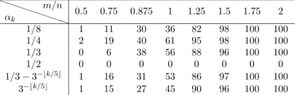
parameter to specify the noise half-width at half-maximum [50, 52, 53], and we also test for a uniformly distributed noisee∼ U(−δ, δ) (i.e., the uniform distribution on the interval (−δ, δ)), whereδ >0 is a noise range parameter [8, 57]. All experiments were performed under Windows Vista Premium and MATLAB v7.8 (R2016b) running on a Huawei laptop with an Intel(R) Core(TM)i5-8250U CPU at 1.8 GHz and 8195MB RAM of memory. 5.1. CAPReaL algorithm with different selection of step sizes. In this subsection, we demonstrate the performance of the CAPReaL algorithm with different selection of step sizes to recover sparse signals from their affine quadratic affine measurements. Shown in Table 1 are average success per-centages of the CAPReaL algorithm for different selection of step sizes over 100 independent realizations to recover sparse signals from their noiseless quadratic measurements of sizem, where the original sparsity signalxo has
sparsitys= 4 and lengthn= 64, and step sizesαk= 1/8,1/4,1/3,1/2 are
independent of k for the first three simulations and αk = 1/3−(1/3)bk/5c
and (1/3)bk/5c, k ≥ 0 for the last two simulations. Here bac denotes the nearest integer less than or equal to a. In the simulation, the recovery is regarded as successful if kx∗−xok2/kxok2 ≤ 0.01, where x∗ is the
recon-structed signal via the CAPReaL algorithm. This indicates that step sizes in the CAPReaL algorithm should be chosen appropriately and the CAPReaL algorithm with step sizeαk = 1/4 for allk≥0 has highest success
percent-age to recover sparse signals from their phaseless affine measurements. Due to the above observation, in the following simulations, we always choose
αk = 1/4, k ≥ 0, as step sizes in the CAPReaL algorithm and also in the p-CAPReaL algorithm.
Table 1. Success percentage of the CAPReaL algorithm to recover sparse real signals over 100 repeated trials for dif-ferent ratios m/n between the number m of measurements and the length of original signals, and for different selections of step sizes αk, k≥0. P P P P P P PP αk m/n 0.5 0.75 0.875 1 1.25 1.5 1.75 2 1/8 1 11 30 36 82 98 100 100 1/4 2 19 40 61 95 98 100 100 1/3 0 6 38 56 88 96 100 100 1/2 0 0 0 0 0 0 0 0 1/3−3−bk/5c 1 16 31 53 86 97 100 100 3−bk/5c 1 15 27 45 90 96 100 100
5.2. Comparison between CAPReaL and Jacobian/twisted ADMM-based algorithms. The proposed CAPReal algorithm to recover sparse real vectors from their affine quadratic measurements is based on the Prox-IADMM. In our simulations, we always select step sizes αk = 1/4, k ≥ 0,
in the CAPReaL algorithm, see Subsection 5.1. As the Prox-IADMM (1.4) with zero step sizes becomes the classical ADMM (1.2), we may use the cor-responding CAPReal algorithm based on the classical ADMM, CAPReaL-Zero for abbreviation, to solve (1.12). Based on the Jacobi-Proximal ADMM [22], we propose the following iterative algorithm, CAPReaL-Jacobi for ab-breviation, to solve (1.12), where η1, η2, η3 are proximal parameters, each
iteration is modified from the proximal Jacobian ADMM [22], xk+1 = S xk−η1BT 1 2A(X k) +1 2A(Y k) +Bxk−c−zk β ,λη1 β , Xk+1 = P Xk−η2 β In− η2 2A ∗ 1 2A(X k) + 1 2A(Y k) +Bxk+1−c−zk β −η2 Xk−Yk−Z k β , Yk+1 = SYk−η3 2A ∗1 2A(X k) +1 2A(Y k) +Bxk+1−c− 1 βz k+1 +η3 Xk−Yk− Zk+1 β ,τ η2 β , zk+1 = zk−β 1 2A(X k+1) + 1 2A(Y k+1) +Bxk+1−yk+1−c, Zk+1 = Zk−β Xk+1−Yk ,
and the compensation step is the same as the one in Subsection 4.1 being used to design the CAPReal algorithm. Similarly, based on twisted version
of the proximal ADMM [54] and following the same compensation step as the one in the CAPReal algorithm, we propose the following iterative algo-rithm, CAPReaL-Twisted for abbreviation, to solve (1.12), whereα∈(0,2), 0 < η2 < (2kBTBk2→2)−1,0 < η3 < 2(kA∗A+ 4InkF→F)−1 are proximal
parameters, and each iteration is essentially the proximal twisted ADMM [54], ˜ Xk=P βA∗A/4 +βIn −1 β Yk+ Z k β −In −β 2A ∗ 1 2A(Y k) +Bxk−c−zk β , ˜ zk=zk−β1 2A( ˜X k) +1 2A(Y k) +Bxk−c, ˜ Zk=Zk−β( ˜Xk−Yk), ˜ xk =S xk−η1BT 1 2A( ˜X k) +1 2A(Y k) +Bxk−c−˜zk β ,λη1 β , ˜ Yk=SYk−η3 2A ∗1 2A( ˜X k) +1 2A(Y k) +Bxk−c− 1 β˜z k +η3 X˜k−Yk− ˜ Zk β ,τ η2 β , Xk+1= ˜Xk, (Yk+1;xk+1;zk+1;Zk+1) = (1−α)(Yk;xk;zk;Zk) +α(Yek;xek;ezk;Zek).
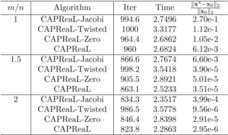
In this subsection, we present some numerical results to compare the per-formance of CAPReaL, Zero, Jacobi and CAPReaL-Twisted algorithms to recover s-sparse real vectors xo ∈ Rn from their quadratic measurement c=|Axo+b|2.
Shown in Table 2 are the average of the iteration number Iter and the time consumptionT ime in seconds to reach the stopping criterion, and the relative reconstruction errorkx∗−x
ok2/kxok2 between the recovered sparse
signal x∗ and the original sparse signal xo over 100 trials for different ratio m/nbetween the numbernof measurements and the lengthnof the original vector, where the original sparsity signal xo has sparsity s= 4 and length n= 64, and the stopping criteria in the compensation step are the same for all algorithms,
kYk−xk(xk)TkF/kxk(xk)TkF ≤ε˜:= 10−5,
cf. (4.4), and the stopping criteria for the ADMM step are
kxk+1−x¯kk2β/η 1I−βBTB+ 2βkXkj+1−X¯kjk2 2 η2 + 2βkYkj+1−Y¯kjk2 2 η3 +3 βkz k+1−¯zkk2 2+ 3 βkX k+1−Z¯kk2 2 ≤:= 10−2
Table 2. Average iteration number and time consumption over 100 trials to implement the proposed algorithms for dif-ferent ratio m/n between the number m of measurements and the lengthnof the original signal.
m/n Algorithm Iter Time kx∗−x0k2
kx0k2 1 CAPReaL-Jacobi 994.6 2.7496 2.70e-1 CAPReaL-Twisted 1000 3.3177 1.12e-1 CAPReaL-Zero 964.4 2.6862 1.05e-2 CAPReaL 960 2.6824 6.12e-3 1.5 CAPReaL-Jacobi 866.6 2.7674 6.60e-3 CAPReaL-Twisted 998.2 3.5418 3.90e-5 CAPReaL-Zero 905.5 2.8921 5.01e-5 CAPReaL 863.1 2.5233 3.51e-5 2 CAPReaL-Jacobi 834.3 2.3517 3.99e-4 CAPReaL-Twisted 986.5 3.5778 9.56e-6 CAPReaL-Zero 846.4 2.8398 2.91e-5 CAPReaL 823.8 2.2863 2.95e-6
for the CAPReaL and CAPReaL algorithms (cf. (2.11)), max kxk−˜xkk 2 1 +kxkk 2 kYk−Y˜kk 2 1 +kYkk 2 ,kz k−˜zkk 2 1 +kzkk 2 ,kZ k−Z˜kk 2 1 +kZkk 2 ≤:= 10−2 for the CAPReaL-Twisted algorithm (cf. [54, Eqn. 51]), and
2βkxkj+1−xkjk2 2 η1 +2βkX k+1 j −Xkjk22 η2 +2βkY k+1 j −Yjkk22 η3 +3−γ βγ2 kz k+1−zkk2 2+ 3−γ βγ2 kZ k+1−Zkk2 2 ≤ς := 10 −2 (5.1)
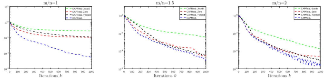
foe the CAPReaL-Jacobi algorithm (cf. [22, Lemma 2.1, Eqn 2.2]). Plotted in Figure 1 is the average of the relative error kxk−x
ok2/kxok2,1 ≤ k ≤
1000, between the reconstructed signalxkin thek-th iteration and the orig-inal sparse signalxo over 100 trials. From Table 2 and Figure 1, we observe
that the proposed CAPReaL algorithm has more favorable performance on the recovery of sparse real vectors from their quadratic measurements than the CAPReaL-Twisted, CAPReaL-Jacobi, and CAPReaL-Zero algo-rithms do.
5.3. Noiseless quadratic measurements. (Sparse) phase retrieval plays an influential role in signal/image/speech processing and it has received con-siderable attention in recent years, see [13, 14, 35] and references therein. A fundamental problem is whether and how a (sparse) vector x ∈ Rn (or
Cn) can be reconstructed from its quadratic measurements c = |Ax|2 = [|aT
0 100 200 300 400 500 600 700 800 900 1000 10-3 10-2 10-1 100 101 CAPReaL-Jocabi CAPReaL-Zero CAPReaL-Twisted CAPReaL 0 100 200 300 400 500 600 700 800 9001000 10-6 10-4 10-2 100 CAPReaL-Jocabi CAPReaL-Zero CAPReaL-Twisted CAPReaL 0 100 200 300 400 500 600 700 800 9001000 10-6 10-4 10-2 100 CAPReaL-Jocabi CAPReaL-Zero CAPReaL-Twisted CAPReaL
Figure 1. The average relative error of kxk−x0k2/kx0k2,
1≤k ≤1000, ink-th iteration over 100 trials in the imple-mentation of the proposed algorithms to reconstruct sparse signals from their quadratic measurements.
Various algorithms have been proposed to recover an (sparse) original sig-nal, up to a trivial ambiguity, from its quadratic measurements, see the survey paper [38] and references therein. By (1.8), the recovery of a signal x ∈ Rn with sparsity s from its affine quadratic measurement |Ax+b|2 reduces to finding a signal ˜xwith sparsitys+ 1 and last component 1 from its quadratic measurement |A˜˜x|2 = |Ax+b|2. Therefore we may adjust
the CPRL algorithm [46, 40], Thresholded Wirtinger flow method (TWF) [9], CoPRAM approach [39] by normalizing the last component to 1 in each iteration through dividing the last component and we denote the adjusted algorithms as CPRLr, TWFr and CoPRAMr respectively. Shown in Table 3
is the success percentage of the proposed CAPReaL algorithm and the ad-justed algorithms CPRLr, TWFr and CoPRAMrto recovers-sparse vectors
in Rn from their quadratic affine measurements of size m, over 100 trials, where s = 4, n = 64 and 1/2 ≤ m/n ≤ 2. This indicates that the pro-posal CAPReaL method has thebestperformance to recover sparse signals from their noiseless affine quadratic measurements, followed close behind by CPRLr and then by TWFr and CoPRAMr. On the other hand, our
simu-lations indicates that TWFr and CoPRAMrconsume much less time in the
implementation than CAPReaL and CPRLr do.
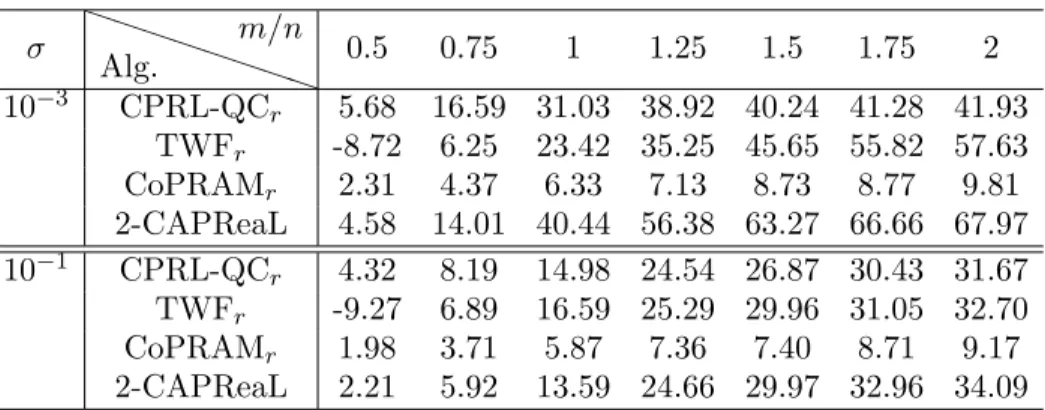
5.4. Quadratic measurements corrupted by Gaussian noises. In this subsection, we demonstrate the performance of 2-CAPReaL algorithm to recover sparse signalsxo∈Rnfrom their quadratic measurements corrupted by Gaussian white noises. For the comparison, we compare the proposed 2-CAPReaL algorithm with adjusted CPRL-QCr, TWFr and CoPRAMr.
Here CPRL-QCr is adjusted from the CPRL-QC algorithm [46],
(5.2a) min
XO tr(X) +τkXk1 subject tokA(X)−ck2 ≤ε,
by normalizing the last entries of the matrix X to 1 in each iteration by dividingXn+1,n+1, whereτ >0 is balancing parameter and ε=kek2 is the
Table 3. Success percentage of the CPRLr, TWFr,
CoPRAMr and CAPReaL algorithms to recover sparse
sig-nals with 100 repeated trials for different ratiosm/nbetween the number m of measurements and lengthn of the original sparse signal. P P P P P P PP Alg. m/n 0.5 0.75 1 1.25 1.5 1.75 2 CPRLr 1 10 62 87 93 96 100 TWFr 0 3 14 33 51 62 70 CoPRAMr 0 1 2 2 3 4 5 CAPReaL 2 19 61 95 98 100 100
Table 4. The average SNR of the CPRL-QCr, TWFr,
CoPRAMr and 2-CAPReaL algorithms to recover sparse
so-lutions over 100 trials for different ratios m/n between the numberm of measurements and the lengthnof original sig-nals and for two different Gaussian noise levelsσ.
σ P P P P P P PP Alg. m/n 0.5 0.75 1 1.25 1.5 1.75 2 10−3 CPRL-QCr 5.68 16.59 31.03 38.92 40.24 41.28 41.93 TWFr -8.72 6.25 23.42 35.25 45.65 55.82 57.63 CoPRAMr 2.31 4.37 6.33 7.13 8.73 8.77 9.81 2-CAPReaL 4.58 14.01 40.44 56.38 63.27 66.66 67.97 10−1 CPRL-QC r 4.32 8.19 14.98 24.54 26.87 30.43 31.67 TWFr -9.27 6.89 16.59 25.29 29.96 31.05 32.70 CoPRAMr 1.98 3.71 5.87 7.36 7.40 8.71 9.17 2-CAPReaL 2.21 5.92 13.59 24.66 29.97 32.96 34.09
noise bound. We use the average of the signal-to-noise ratio (SNR) in dB, (5.3) SNR(x∗,xo) = 20 log10
kxok2
kx∗−x
ok2 ,
over 100 independent trials as our performance measure, where x∗ is the reconstructed signal. Shown in Table 4 is the result of our proposed 2-CAPReaL algorithm to recover sparse signals from their quadratic affine measurements and the performance comparison with the CPRL-QCr, TWFr
and CoPRAMr, where the Gaussian white noise levelσ = 10−3,10−1. This
shows that for m/n ≥1, the proposal 2-CAPReaL is more robust against Gaussian white noises than the CPRL-QCr, TWFr and CoPRAMr do
es-pecially when the noise level is low, while form/n <1 the CPRL-QCr has
Table 5. The average SNR of the CPRL-LADCr, TWFr,
CoPRAMr and 1-CAPReaL algorithms to recover sparse
sig-nals from their quadratic affine measurements corrupted by Cauchy noises over 100 trials for different ratiosm/n and for two different Cauchy noise levels γ.
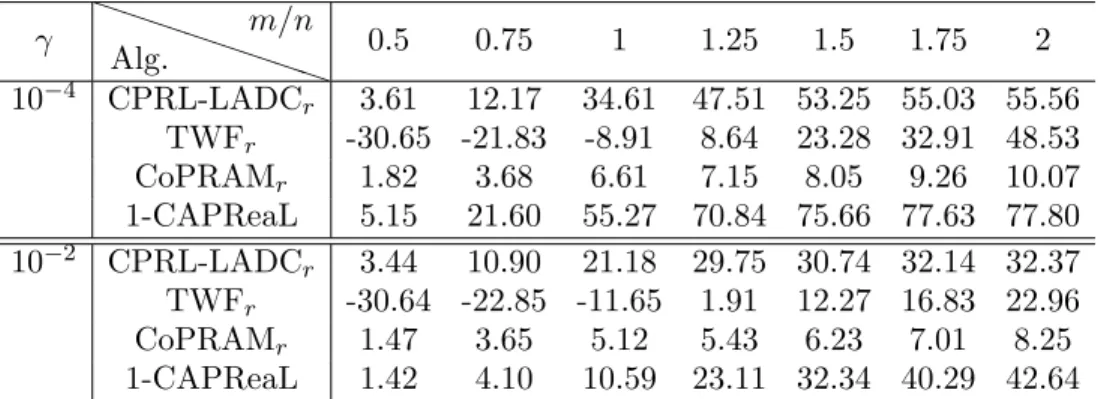
γ P P P P P P PP Alg. m/n 0.5 0.75 1 1.25 1.5 1.75 2 10−4 CPRL-LADCr 3.61 12.17 34.61 47.51 53.25 55.03 55.56 TWFr -30.65 -21.83 -8.91 8.64 23.28 32.91 48.53 CoPRAMr 1.82 3.68 6.61 7.15 8.05 9.26 10.07 1-CAPReaL 5.15 21.60 55.27 70.84 75.66 77.63 77.80 10−2 CPRL-LADCr 3.44 10.90 21.18 29.75 30.74 32.14 32.37 TWFr -30.64 -22.85 -11.65 1.91 12.27 16.83 22.96 CoPRAMr 1.47 3.65 5.12 5.43 6.23 7.01 8.25 1-CAPReaL 1.42 4.10 10.59 23.11 32.34 40.29 42.64
5.5. Quadratic measurements corrupted by impulsive noises. For the case that quadratic measurements are corrupted by the impulsive Cauchy noise, we will use the p-CAPReaL algorithm with p = 1 to recover sparse signals from their corrupted quadratic measurements. Presented in Table 5 are performances of CPRL-LADCr, TWFr, CoPRAMr and 1-CAPReaL
algorithms to recover sparse solutions for different ratios m/n between the numbermof measurements and the lengthnof original signals, and for two different Cauchy noise levels γ, where CPRL-LADCr is modified from the
CPRL-LADC algorithm, (5.4a) min
XO tr(X) +τkXk1 subject tokA(X)−ck1 ≤ε,
by adjusting the last entries of the matrix X to one in each iteration by dividing Xn+1,n+1, where τ > 0 is balancing parameter and ε = kek1 is
noise bound. Therefore for the recovery of sparse signals from their affine quadratic measurements corrupted by the impulsive noise of Cauchy type, the CPRL-LADCr and the proposed 1-CAPReaL have much better
perfor-mance than TWFr and CoPRAMr do, the CPRL-LADCr achieves higher
SNR than the 1-CAPReaL does when we have less measurements and the 1-CAPReaL does better job than CPRL-LADCr does when we have more
measurements.
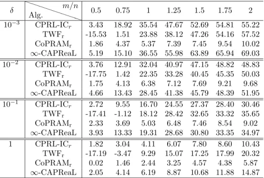
5.6. Quadratic measurements corrupted by bounded noises. In this subsection, we approximate the true sparse signal xo when its quadratic
measurements are corrupted by a uniformly distributed noise with different noise boundδ. Shown in Table 6 is the performances of CPRL-ICr, TWFr,