Pham-Meyer-2016

(1)

Study of Meta-Analysis Strategies for Network Inference using

Information-Theoretic Approaches

Ngoc Cam Pham∗, Benjamin Haibe-Kains†, Pau Bellot‡, Gianluca Bontempi§ and Patrick E. Meyer∗ ∗_{Bioinformatics and Systems Biology (BioSys) Unit, Universit´e de Li`ege, Belgium}

†_{Princess Margaret Cancer Centre, University Health Network, Toronto, Canada} ‡_{Image Processing group, Technical University of Catalonia, Spain}

§_{Machine Learning Group, Interuniversity Institute of Bioinformatics in Brussels (IB)}2_{, Universit´e Libre de Bruxelles, Belgium}

Abstract—Reverse engineering of gene regulatory networks (GRNs) from gene expression data is a classical challenge in systems biology. Thanks to high-throughput technologies, a massive amount of gene-expression data has been accumulated in the public repositories. Modelling GRNs from multiple experiments (also called integrative analysis) has; therefore, naturally become a standard procedure in modern computa-tional biology. Indeed, such analysis is usually more robust than the traditional approaches focused on individual datasets, which typically suffer from some experimental bias and a small number of samples.

To date, there are mainly two strategies for the problem of interest: the first one (”data merging”) merges all datasets together and then infers a GRN whereas the other (”networks ensemble”) infers GRNs from every dataset separately and then aggregates them using some ensemble rules (such as ranksum or weightsum). Unfortunately, a thorough comparison of these two approaches is lacking.

In this paper, we evaluate the performances of various meta-analysis approaches mentioned above with a systematic set of experiments based on in silicobenchmarks. Furthermore, we present a new meta-analysis approach for inferring GRNs from multiple studies. Our proposed approach, adapted to methods based on pairwise measures such as correlation or mutual information, consists of two steps: aggregating matrices of the pairwise measures from every dataset followed by extracting the network from the meta-matrix.

Keywords-Meta-analysis, gene regulatory networks, systems biology, gene expression, mutual information.

I. INTRODUCTION

One of the most long-standing challenges in Systems Biology is the development of methods, which are able to construct the complete set of regulatory interactions of a cell. The regulating circuitry, also called gene regulatory network (GRN), can then be used by bio-medical experts to understand key mechanisms in cells. Thanks to high-throughput technologies, a large amount of transcriptome data is now available through public repositories (e.g. NCBI GEO [1], ArrayExpress [2]), providing opportunities to study the GRNs of many organisms. In the last decade, a variety of methods have been proposed in an attempt to address this reverse engineeringproblem. The methods can

be classified into several categories [3], such as: regression-based, pairwise similarity (mutual information, correla-tion,...), Bayesian networks or even ensemble approaches (that combine several different approaches). Among those, mutual information (MI) based methods, such as CLR [4], ARACNE [5], MRNET [6], [32] and so on, gather more and more attention due to their capability to deal with up to several thousands of variables in the presence of a limited number of samples [6]. Generally, these methods first estimate a pairwise mutual information (i.e. a non-linear dependency measure) between all pairs of genes, resulting in a mutual information matrix (MIM). Afterwards, indirect interactions are eliminated from the MIM by the different methods and thus a GRN is inferred.

Since a single dataset has typically a small sample size (usually less than 200 observations) and suffers from po-tential experimental biases, classical analytical tools show their limits in unravelling reliably underlying interactions. By contrast, integrative analysis of multiple studies is able to increase significantly the statistical power and thus is becoming a standard procedure in modern computational biology [7]. However, the question of integrating all the data consistently and efficiently raises new questions [8].

(2)

model. If the problem of detecting differentially expressed genes across several studies has been intensively studied, it is, however, not yet the case when it comes to constructing GRNs.

To deal with this challenge of meta-network inference, there have been plenty of proposed methods, which can be divided into two main categories: data merging and network ensemble. In the data merging approach, datasets are integrated at the expression level into a unique dataset, from which GRNs are inferred [9]–[11]. However, one of the major problem of this approach is the removal of batch effects. Indeed, the use of different platforms, and different methodologies by different research groups introduce statistical biases (batch effects) that can lead to incorrect conclusions [12]. For example, it is known that normalization techniques, such as RMA [13], consisting in re-scaling gene expression values at the probe intensity level for Affymetrix data [14], is not able to remove batch effects. Consequently, batch removal methods, like COMBAT [15], is typically used before merging data [12]. The approach consists in merging GRNs from different datasets, for exam-ple by weighting gene-gene interactions according to their average rank in each network [3]. This approach rooted in the ”wisdoms of crowds” concept, which was first introduced in the DREAM5 challenge and then further developed by [16] with the TopkNet algorithms to produce consensus networks.

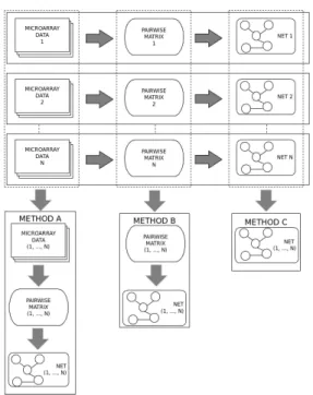
In this paper, we also introduce a new meta-analysis strategy to build a consensus network. The new strategy con-sists in aggregating matrices of pairwise mutual information with each being estimated from a gene expression dataset to produce a meta-matrix, from which a GRN is inferred using classical information-theoretic network inference al-gorithms. Additionally, the paper presents the first thorough experimental comparison of these three ”meta” approaches for the reconstruction of networks, namely data merging, network ensemble and coexpression matrices aggregation. The performances of these three sets of methods are evalu-ated using synthetic datasets from the standard Bioconductor netbenchmark package.

II. METHODS A. State-of-the-art

Mutual information is a non-linear measure of dependency between two variables (genes) X andY, defined as follow

I(X, Y) = X

x⊂X,y⊂Y

p(x, y)log p(x, y)

p(x)p(y) (1)

where p(x, y) is the joint probability distribution of X

and Y, and p(x) and p(y) are the marginal probability distributions ofX andY, respectively.

This dependency measure has been used for reconstruct-ing networks by several methods such as CLR, ARACNE or

Figure 1: Meta-network strategies: assembling datasets, pairwise matrices or networks

MRNET. The Context Likelihood or Related network (CLR) method [4] creates an edge between each pair of genesiand

jif the combined z-score of the mutual information between them is above a given threshold, where the combined z-score is defined as:

cij=qc2

i +c2j withci= max(0,

Mij−µM_i σM_i ) (2)

in which,µMi andσMi are the mean and standard deviation of the empirical distribution of the mutual information of genei.

The Algorithm for the Reconstruction of Accurate Cellu-lar Networks (ARACNE) [5], relies on the ”Data Processing Inequality” (DPI) which removes the edge with the weakest mutual information, in every triplet of genes.

Finally, the Minimum Redundancy NETworks (MRNET) [6], [32] method reconstructs a network using the feature selection technique known as Minimum Redundancy Max-imum Relevance (MRMR) [23]. The minMax-imum redundancy criterion makes the implicit assumption that variables with redundant information to the most relevant variables are indirect links.

Using those three information-theoretic network inference techniques, available in the Bioconductor Minet package, we will compare three meta-analysis approaches detailed in the next sections.

B. Data merging - A methods

(3)

named data merging and denoted here with the letter (A), were widely used in [9]–[11] to reconstruct large-scale GRNs because of their simplicity. However, since high di-mensional data often suffers from unwanted biases, a variety of techniques can be used to correct for these non-biological variations. We present in the following two classical scaling methods typically used to assemble datasets, and one batch-effect-removal method.

1) Normalization: BMC(A1) and z-score (A2): LetX be a matrix Xm×n _{denoting the dataset of gene expression}

values. In this matrix, columns represent samples and rows represent genes, and xij represents the expression value of gene i in sample j of dataset X. In [24], a normalization technique named BMC (equation 3) was applied for merging breast cancer datasets.

ˆ

xij =xij−x¯i (3)

Similarly, the z-score normalization [25] described by equa-tion 4 can be also performed.

ˆ

xij =xij−x¯i

σx_i (4)

2) Batch effects removal: COMBAT(A3): Expression datasets mostly come from different platforms and labora-tories, causing the so-called ’batch effects’. Consequently, batch removal methods, like COMBAT (also known as Empirical Bayes) [15], is often used to detect and remove this inevitable variation. COMBAT, which was shown to outperform other commonly used batch removal methods in some specific scenarios [26], uses estimations for the LS (location-scale) parameters (e.x. mean and variance) for each gene independently [27]. The gene, afterwards, is adjusted to meet the estimated model.

C. Networks ensemble - C methods

The second category of approaches for integrative analysis (networks ensemble - denoted with the letter (C) in this paper) first constructs every single transcriptional networks independently before combining them to produce a so-called community network [3]. In general, combining networks consists in two distinct steps: transformation and aggrega-tion [28]. Indeed, before assembling networks, a network-normalization step is also performed because it is common to observe networks that exhibit different distribution of edge weights.

Let eij be the weight of an edge between gene i and gene j and tn(eij) be the normalized value for eij in the networkn. In the next subsections, we discuss three different combinations of network transformation and aggregation.

1) No normalization and aggregation with the sum rule(C1): In this approach, all networks are simply com-bined together using the sum rule

aN O(eij) =

N

X

n=1

eij (5)

withaN O(eij)denoting the aggregated score in the ensem-ble network.

2) Normalization with z-score and aggregation with the sum rule(C2): Z-score transformation, the well-know nor-malization strategy for merging data mentioned in the pre-vious section, can also be applied for ensemble networks. It is worth emphasizing that datasets are normalized by vari-ables/columns whereas networks are edge lists normalized “globally”, i.e. as a single vector of weights.

tn(eij) =sn(eij) (6) Here,sn(eij)denotes the z-score transformation of the edge

eij. After normalization, all the network can be combined using the sum rule.

aZ(eij) =

N

X

n=1

tn(eij) (7)

3) Median method (C3): In [16] the median value was introduced for aggregating consensus networks. This method assigns the median value amongN values representing the confidence score of a specific edge inN different networks.

aM(eij) =median{t1(eij), ..., tN(eij)} (8) D. Coexpression matrices aggregation approaches - B meth-ods

Our new category of meta-analysis approaches (denoted with the letter (B) in this paper) aggregates mutual informa-tion matrices rather than data or networks. The idea behind assembling pairwise matrices is that, although expression data typically shows high variability due to differences in technology, samples, labels, etc., pairwise dependency measures between genes should be much less variant (i.e. dependent variables, such as a regulating variable and its regulated counterpart, should remain dependent in every platform/experiment/dataset even if ranges of values differ greatly). Thus, to infer a network from various expression data, our approach consists in combining mutual information matrices (MIMs) estimated independently from each dataset. Then a GRN network is inferred from the aggregated MIMs. In the following subsections, we compare three methods to assemble matrices of pairwise measure.

(4)

random-effects method, but using MI instead of correlations.

ˆ

IRE(X;Y) =

N

P

k=1

nkI(Xk;Yk)

N

P

k=1

nk

(9)

whereI(Xk;Yk)is the MI between two variableXk andYk

in the studykandnk is the number of samples of study k. The idea is simply that effect sizes based on large samples will be more precise than those based on small samples.

2) Median method (B2): One of the major issue of B1 is that the quality of datasets used in meta-analysis is not explicitly taken into account. Indeed, inclusion of a noisy datasets is likely to weaken statistical power [17]. Thus, an alternative schema for combining MIMs across heteroge-neous studies, namely method B2 can be proposed. Method B2 is explained by formula 10, in which the aggregated MI of a gene pairX andY is the median value of all MI values between them across all studies.

ˆ

IM(X, Y) =median(I(X1, Y1), I(X2, Y2), ...I(XN, YN)) (10) 3) Internal quality control index (B3): In [17], six quan-titative quality control measures have been proposed for the inclusion/exclusion of gene expression studies used for the meta-analysis. Among these measures, the internal quality control index will be used, as method B3 for assembling matrices. Let the similarity between two studiesmandnbe defined as

rmn=spcor((Imij; 1≤i≤j≤G),(Inij; 1≤i≤j≤G)) (11) In which rmn is the Spearman’s rank correlation of the pairwise correlation structure between study m and n and

Grepresents the total number of genes in the studies. The dissimilarity (or distance) between studymandnis defined as dmn= (1−rmn)/2. For a given studyk, a weight -wk

will be granted as the fraction between the sum of distances between study k - D_k∗ to all other studies and the sum of pairwise distances between all studies excluding the study

k- D#_k with

D_k∗={dkn}1≤n≤N;n6=k andD_k#={dmn}1≤m6=n≤N;m6=k;n6=k

(12) Afterwards, the MI between two variables (genes)X andY

is aggregated by the following equation:

ˆ

IIQC(X;Y) =

N

P

k=1

wkI(Xk;Yk)

N

P

k=1

wk

(13)

III. EXPERIMENTS A. Data collection and benchmarking process

There are two tasks one needs to consider in order to validate networks: 1) defining a ”gold standard” - which is a

set of true regulations describing the underlying interaction network, 2) selecting quantitative measures to statistically assess the quality of inferred networks. Typically, the first task is addressed by collecting well-known regulations mined from literature with strong supporting evidences. However, those regulations just cover a small part of the underlying network and hence cannot be an ideal reference network to thoroughly compare methods. Hence the latter approach is often completed byin-silico experiments.

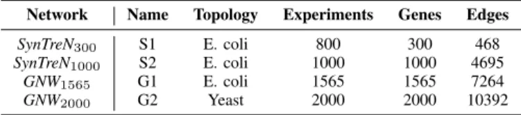
In this paper,in silicobenchmarks are selected from every one of the 4 biological networks and artificially generated datasets coming from the Netbenchmark Bioconductor pack-age [31]. The characteristics of the 4 networks are shown below in the table I.

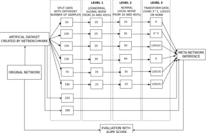
Each large dataset will be split into 6 sub-datasets with a number of experiments ranging between 30 to 300 (a number chosen randomly in order to simulate real case scenario). For example, in Figure 3, an original dataset is split into 6 sub-datasets with the following number of samples: 50, 100, 150, 120, 70 and 190. Additionally, two extremely noisy studies are added, both with a large sample size for each (between 280 and 300). Those datasets allow to test the sensitivity of meta-network methods to datasets that should typically be excluded. Indeed, a few biological studies dating back to the beginning of the microarray technology have very little information and are typically excluded from meta-analysis studies. In order to make the network inference problem

Table I: Networks used in the paper

Network Name Topology Experiments Genes Edges

SynTreN300 S1 E. coli 800 300 468

SynTreN1000 S2 E. coli 1000 1000 4695

GNW1565 G1 E. coli 1565 1565 7264 GNW2000 G2 Yeast 2000 2000 10392

more challenging and realistic, noise and transformations of data are added. In particular, we define three levels of data-distortion: i) Level 1: An independent lognormal noise call “global” noise, with intensity between 20 and50%, is added to the first 6 datasets. The standard deviation of this noise (σGlobal) is the same for the whole data set and is a percentage (κg%) of the mean variance of all the genes in the dataset(σg¯). It is defined as follows: σGlobal;κg% =

¯

σg

U(0.8κ,1.2κ)

100 .ii) Level 2: In addition to the global noise, a normally distributed “local” noise with intensity also ranging between20and50%, is added. This is an additive Gaussian noise with zero mean and a standard deviation (σLocal(g)) that is around a percentage (κ%) of the gene standard deviation (σg). Therefore, the Signal-to-Noise-Ratio(SNR) of each gene is similar. The local noise standard deviation can be formulated as follows:σLocal(g);κ%=σg

(5)

Figure 2: Framework for data collection, network predic-tion and validapredic-tion

non-linear transformation such asx2orlog(x). This random data transformation is not really meant to be realistic but rather to allow us to better assess the behaviour of each meta-method when faced with extreme distortion. It is worth emphasizing that the two non-informative studies remain un-changed across all experiments. A flowchart of this process is illustrated in Figure3.

B. Network prediction and validation

The schema for network prediction and validation is also illustrated in Figure3. Initially, all methods (three A, B and C, totalling nine) are used to construct a consensus GRN from the split datasets. All methods are assessed on 12 challenges (three levels of distortion for four datasets). Finally, the process is repeated for the three information-theoretic inference methods, hence totalling 36 challenges. This is done to make sure that our analysis is not method specific. In this study, the Area Under Precision Recall (AUPR) of each GRN is calculated for all methods in each challenge. Due to the randomization of various experimental parameters (noise intensity, number of samples), 10 repeti-tions are made. Finally, the average of the ten AUPR values, for each method on each challenge, is reported.

IV. RESULTS ANDDISCUSSION

In this section, we present the experimental results of all presented methods for reconstructing GRNs from multiple expression datasets (Table II). For the A family of methods, it can be observed that normalization using z-score transfor-mation (A2) is better than BMC (A1). This conclusion is true for all three network inference algorithms used in this paper, namely MRNET, ARACNE and CLR. Another striking fea-ture is that batch effect removal methods like COMBAT (A3) is able to increase significantly the robustness of network inference algorithms. The results reinforce the idea that normalization alone can not remove batch effects. In the

case of method C, there are no clear differences between C1, C2 or C3, except when using ARACNE-C3.

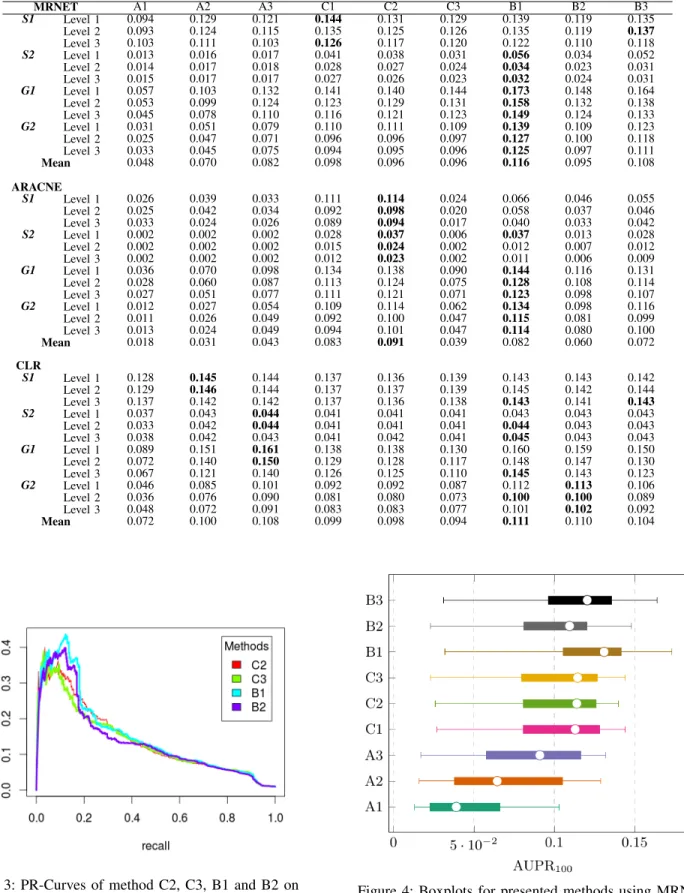
Interestingly, we can clearly observe that all three C meth-ods outperform all three A methmeth-ods suggesting that assem-bling networks is better than merging datasets. This could be explained by the fact that gene expression values are very dissimilar in various experiments due to our simulated batch effects (i.e. datasets with different global and local noise). However, the particular combination CLR - A3 offers an exception to this observation. It also should be noted that assembling mutual information matrices (B methods) surpasses the two other well-known strategies (A and C) for all datasets under every different levels of distortion, in particular for MRNET and CLR. Experimental results also suggest that MRNET benefits the most from meta-analysis and CLR appears to be the most robust. This suggests that while CLR might be a better strategy for analazing individual datasets, MRNET might be a better choice when multiple datasets are available. Although ARACNE appears to be much worse than the two other techniques, that is mainly due to a bad recall (though not visible with AUPR numbers, its precision remains quite competitive). Finally, in the B family of methods, it appears that combining MIM using random effect model (B1) is better than the two other strategies, the median method (B2) and the internal quality control index (B3).

V. CONCLUSION

(6)

Table II: Area under PR-Curves (the higher the better) for 9 methods on 4 datasets with 3 levels of increasing data-distortion.

MRNET A1 A2 A3 C1 C2 C3 B1 B2 B3

S1 Level 1 0.094 0.129 0.121 0.144 0.131 0.129 0.139 0.119 0.135 Level 2 0.093 0.124 0.115 0.135 0.125 0.126 0.135 0.119 0.137 Level 3 0.103 0.111 0.103 0.126 0.117 0.120 0.122 0.110 0.118

G1 Level 1 0.057 0.103 0.132 0.141 0.140 0.144 0.173 0.148 0.164 Level 2 0.053 0.099 0.124 0.123 0.129 0.131 0.158 0.132 0.138 Level 3 0.045 0.078 0.110 0.116 0.121 0.123 0.149 0.124 0.133

G2 Level 1 0.031 0.051 0.079 0.110 0.111 0.109 0.139 0.109 0.123 Level 2 0.025 0.047 0.071 0.096 0.096 0.097 0.127 0.100 0.118 Level 3 0.033 0.045 0.075 0.094 0.095 0.096 0.125 0.097 0.111 Mean 0.048 0.070 0.082 0.098 0.096 0.096 0.116 0.095 0.108

ARACNE

CLR

Figure 3: PR-Curves of method C2, C3, B1 and B2 on

(7)

REFERENCES

[1] R. Edgar, M. Domrachev, and A. E. Lash, “Gene expression omnibus: Ncbi gene expression and hybridization array data repository,” Nucleic acids research, vol. 30, no. 1, pp. 207– 210, 2002.

[2] A. Brazma, H. Parkinson, U. Sarkans, M. Shojatalab, J. Vilo, N. Abeygunawardena, E. Holloway, M. Kapushesky, P. Kem-meren, G. G. Lara,et al., “Arrayexpress—a public repository for microarray gene expression data at the ebi,”Nucleic acids research, vol. 31, no. 1, pp. 68–71, 2003.

[3] D. Marbach, J. C. Costello, R. K¨uffner, N. M. Vega, R. J. Prill, D. M. Camacho, K. R. Allison, M. Kellis, J. J. Collins, G. Stolovitzky, •et al., “Wisdom of crowds for robust gene network inference,”Nature methods, vol. 9, no. 8, pp. 796–804, 2012.

[4] J. J. Faith, B. Hayete, J. T. Thaden, I. Mogno, J. Wierzbowski, G. Cottarel, S. Kasif, J. J. Collins, and T. S. Gardner, “Large-scale mapping and validation of escherichia coli transcriptional regulation from a compendium of expression profiles,”PLoS biology, vol. 5, no. 1, p. e8, 2007.

[5] A. A. Margolin, I. Nemenman, K. Basso, C. Wiggins, G. Stolovitzky, R. D. Favera, and A. Califano, “Aracne: an algorithm for the reconstruction of gene regulatory networks in a mammalian cellular context,”BMC bioinformatics, vol. 7, no. Suppl 1, p. S7, 2006.

[6] P. E. Meyer, F. Lafitte, and G. Bontempi, “Minet: An open source r/bioconductor package for mutual information based network inference,”BMC Bioinformatics, vol. 9, 2008.

[7] K. G. Kugler, L. A. Mueller, A. Graber, and M. Dehmer, “In-tegrative network biology: graph prototyping for co-expression cancer networks,”PLoS One, vol. 6, no. 7, p. e22843, 2011.

[8] J. Taminau, S. Meganck, C. Lazar, D. Steenhoff, A. Coletta, C. Molter, R. Duque, V. de Schaetzen, D. Y. W. Sol´ıs, H. Bersini,et al., “Unlocking the potential of publicly avail-able microarray data using insilicodb and insilicomerging r/bioconductor packages,”BMC bioinformatics, vol. 13, no. 1, p. 335, 2012.

[9] W. Huber, A. Von Heydebreck, H. S¨ultmann, A. Poustka, and M. Vingron, “Variance stabilization applied to microarray data calibration and to the quantification of differential expression,”

Bioinformatics, vol. 18, no. suppl 1, pp. S96–S104, 2002.

[10] V. Belcastro, V. Siciliano, F. Gregoretti, P. Mithbaokar, G. Dharmalingam, S. Berlingieri, F. Iorio, G. Oliva, R. Pol-ishchuck, N. Brunetti-Pierri,et al., “Transcriptional gene net-work inference from a massive dataset elucidates transcrip-tome organization and gene function,”Nucleic acids research, vol. 39, no. 20, pp. 8677–8688, 2011.

[11] P. Adler, R. Kolde, M. Kull, A. Tkachenko, H. Peterson, J. Reimand, and J. Vilo, “Mining for coexpression across hundreds of datasets using novel rank aggregation and visu-alization methods,”Genome biology, vol. 10, no. 12, p. R139, 2009.

[12] J. T. Leek, R. B. Scharpf, H. C. Bravo, D. Simcha, B. Lang-mead, W. E. Johnson, D. Geman, K. Baggerly, and R. A. Irizarry, “Tackling the widespread and critical impact of batch effects in high-throughput data,” Nature Reviews Genetics, vol. 11, no. 10, pp. 733–739, 2010.

[13] R. A. Irizarry, B. Hobbs, F. Collin, Y. D. Beazer-Barclay, K. J. Antonellis, U. Scherf, and T. P. Speed, “Exploration, normalization, and summaries of high density oligonucleotide array probe level data,”Biostatistics, vol. 4, no. 2, pp. 249–264, 2003.

[14] L. Dyrskjøt, M. Kruhøffer, T. Thykjaer, N. Marcussen, J. L. Jensen, K. Møller, and T. F. Ørntoft, “Gene expression in the urinary bladder a common carcinoma in situ gene expression signature exists disregarding histopathological classification,”

Cancer Research, vol. 64, no. 11, pp. 4040–4048, 2004.

[15] W. E. Johnson, C. Li, and A. Rabinovic, “Adjusting batch effects in microarray expression data using empirical bayes methods,”Biostatistics, vol. 8, no. 1, pp. 118–127, 2007.

[16] T. Hase, S. Ghosh, R. Yamanaka, and H. Kitano, “Harnessing diversity towards the reconstructing of large scale gene regula-tory networks,”PLoS Comput Biol, vol. 9, no. 11, p. e1003361, 2013.

[17] D. D. Kang, E. Sibille, N. Kaminski, and G. C. Tseng, “Metaqc: objective quality control and inclusion/exclusion criteria for genomic meta-analysis,” Nucleic acids research, vol. 40, no. 2, pp. e15–e15, 2012.

[18] A. Ramasamy, A. Mondry, C. C. Holmes, and D. G. Altman, “Key issues in conducting a meta-analysis of gene expression microarray datasets,” PLoS medicine, vol. 5, no. 9, p. e184, 2008.

[19] P. Wirapati, C. Sotiriou, S. Kunkel, P. Farmer, S. Pradervand, B. Haibe-Kains, C. Desmedt, M. Ignatiadis, T. Sengstag, F. Schutz, et al., “Meta-analysis of gene expression profiles in breast cancer: toward a unified understanding of breast cancer subtyping and prognosis signatures,” Breast Cancer Res, vol. 10, no. 4, p. R65, 2008.

[20] C. Desmedt, B. Haibe-Kains, P. Wirapati, M. Buyse, D. Larsi-mont, G. Bontempi, M. Delorenzi, M. Piccart, and C. Sotiriou, “Biological processes associated with breast cancer clinical outcome depend on the molecular subtypes,”Clinical Cancer Research, vol. 14, no. 16, pp. 5158–5165, 2008.

[21] F. Hong, R. Breitling, C. W. McEntee, B. S. Wittner, J. L. Nemhauser, and J. Chory, “Rankprod: a bioconductor package for detecting differentially expressed genes in meta-analysis,”

Bioinformatics, vol. 22, no. 22, pp. 2825–2827, 2006.

[22] V. Cestarelli, G. Fiscon, G. Felici, P. Bertolazzi, and E. Weitschek, “Camur: Knowledge extraction from rna-seq cancer data through equivalent classification rules,” Bioinfor-matics, p. btv635, 2015.

(8)

[24] A. H. Sims, G. J. Smethurst, Y. Hey, M. J. Okoniewski, S. D. Pepper, A. Howell, C. J. Miller, and R. B. Clarke, “The removal of multiplicative, systematic bias allows integration of breast cancer gene expression datasets–improving meta-analysis and prediction of prognosis,”BMC medical genomics, vol. 1, no. 1, p. 1, 2008.

[25] C. Cheadle, M. P. Vawter, W. J. Freed, and K. G. Becker, “Analysis of microarray data using z score transformation,”

The Journal of molecular diagnostics, vol. 5, no. 2, pp. 73–81, 2003.

[26] C. Chen, K. Grennan, J. Badner, D. Zhang, E. Gershon, L. Jin, and C. Liu, “Removing batch effects in analysis of expression microarray data: an evaluation of six batch adjustment meth-ods,”PloS one, vol. 6, no. 2, p. e17238, 2011.

[27] C. Lazar, S. Meganck, J. Taminau, D. Steenhoff, A. Coletta, C. Molter, D. Y. Weiss-Sol´ıs, R. Duque, H. Bersini, and A. Now´e, “Batch effect removal methods for microarray gene expression data integration: a survey,” Briefings in bioinfor-matics, p. bbs037, 2012.

[28] P. Bellot Pujalte, P. J. Salembier Clairon, A. Oliveras Verg´es, and P. Meyer, “Study of normalization and aggregation ap-proaches for consensus network estimation,” in IEEE SSCI 2015: 2015 IEEE Symposium Series on Computational Intelli-gence; 7-10 December 2015, Cape Town, South Afrika, pp. 1– 6, Institute of Electrical and Electronics Engineers (IEEE), 2015.

[29] K. Wang, M. Narayanan, H. Zhong, M. Tompa, E. E. Schadt, and J. Zhu, “Meta-analysis of inter-species liver co-expression networks elucidates traits associated with common human diseases,” PLoS Comput Biol, vol. 5, no. 12, p. e1000616, 2009.

[30] F. L. Schmidt and J. E. Hunter, Methods of meta-analysis: Correcting error and bias in research findings. Sage publica-tions, 2014.

[31] P. Bellot, C. Olsen, P. Salembier, A. Oliveras-Verges, and P. E Meyer, “Netbenchmark: A bioconductor package for re-producible benchmarks of gene regulatory network inference,”

BMC bioinformatics, 16.1 (2015): 1.