Bono de Desarrollo Humano’s (BDH) Impact on School Enrollment1
1. Introduction
This note presents a preliminary analysis of BDH‘s effect on school enrollment using the propensity score matching method proposed by Dehejia and Wahba [2002]. Our results suggest that BDH had a positive statistically and economically significant effect on the percentage of 5 to 19 year olds who were enrolled in school in 2007. In particular, the estimated enrollment impact for recipient households (the average treatment effect on the treated) is about 0.04, which compares to an enrollment rate of about 78% in the comparison group. We show that the matching procedure we use is quite successful in balancing observable household characteristics that are correlated with school enrollment thus alleviating an important source of bias in our impact estimates.
Whether our estimates represent true causal effects hinges on the untestable assumption that conditional on the covariates we include in our analysis, BDH assignment is as good as random program assignment. This is a particularly strong assumption in our context because, conditional on covariates, either all households or none in a given stratum should have received the BDH according to the program‘s design. More specifically, a household with baseline covariates Xi
should have received treatment T (the BDH) if and only if the Selben score S(Xi) was below the
second quintile of the Selben score distribution S2, i.e. Ti=1[S(Xi)<S2]. Our matching procedure
therefore necessarily compares households that complied with treatment assignment to those that did not.2 If the reasons for differential compliance conditional on covariates are systematically related to enrollment outcomes, our treatment effect estimates will be biased. That is, if some unobserved household characteristic determines, after we have controlled for observable factors, both whether or not the household joins or does not join the BDH program and also whether or not the household enrolls its children in school, then the treatment effect estimated through propensity score matching cannot be said to be unique to the BDH treatment. Figure 1 illustrates the problem.
2. Data source and coding
All variables used for this analysis are constructed from the SIEH-ENEMDU 2007 survey. Because BDH assignment was based on household characteristics, rather than personal
1
Prepared by Stephan Litschig and Matthew S. Winters, Columbia University IGERT Program on International Development and Globalization.
2
characteristics, we conduct our analysis at the level of the household. In order to include personal characteristics of household members in the analysis we aggregate individual responses to the household level. Our treatment variable is coded as 1 if any household member reports to be a BDH recipient.3 Our main outcome variable of interest is the percentage of 5 to 19 year olds per household who were enrolled in school in 2007. Details of the coding procedure are found in the data appendix. Other age ranges and outcome variables such as labor market outcomes could and should be investigated in an extension of this draft.
3. Estimation approach
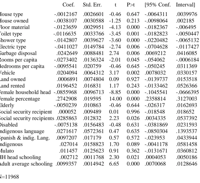
Our estimation approach is based on the algorithm proposed by Dehejia and Wahba [2002] and implemented in Stata as ‗psmatch2‘.4 We start by running a probit model on those Selben variables available in the 2007 survey that were unlikely to have changed significantly since 2003 when the Selben index was first used to target the BDH. The data appendix lists these variables and our coding of the survey data for estimation purposes. Next, we match treatment units to their closest counterpart in the comparison group based on the estimated propensity score (single nearest neighbor matching). We allow for comparison units to be used more than once (replacement). We then use t-tests to evaluate whether ―baseline‖ covariates are balanced across treatment and comparison groups in the matched sample. Although we ensure balance across all baseline covariates, we report balance only on those covariates that are correlated with school enrollment since these are most likely to bias our impact estimates if they are not balanced. (Table I provides the results of a linear regression of the outcome variable on all pre-treatment covariates.)
Balancing checks are carried out for the entire matched sample and for individual propensity score strata to ensure thorough balance. When the tests for individual strata reveal statistically significant mean differences for several strata and/or covariates we add higher order terms of significant predictors to the probit specification and re-evaluate. We also improve balance by dropping treatment units that have no ―close‖ match in the comparison group (caliper matching). In order to remove potential bias due to remaining systematic differences in observed characteristics, we also run OLS regressions with baseline covariates in the matched samples.
4. Estimation results
Table IIa presents estimation results of the average treatment effect on the treated (ATT) using the matching estimator (the average enrollment difference between matched treatment and comparison units) and then OLS with covariates in the matched sample. The probit equation includes linear and selected quadratic terms of the Selben variables. Point estimates are virtually
3
Because BDH is provided to individuals such as the mothers of school-aged children, the elderly and the disabled, it is possible for more than one individual in a household to receive the program. In the 2007 SIEH-ENEMDU survey data, there are 5,814 households receiving BDH and 13,119 households not receiving BDH. Of the 5,814 recipients, 5,250 households report receiving only one subsidy, 519 report two, 38 report three, 6 report four and 1 reports five.
4
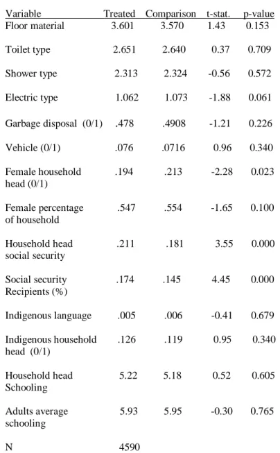
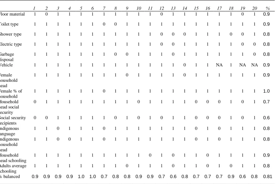
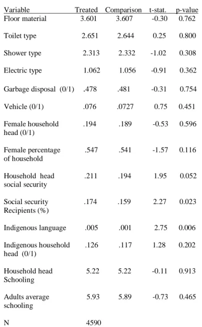
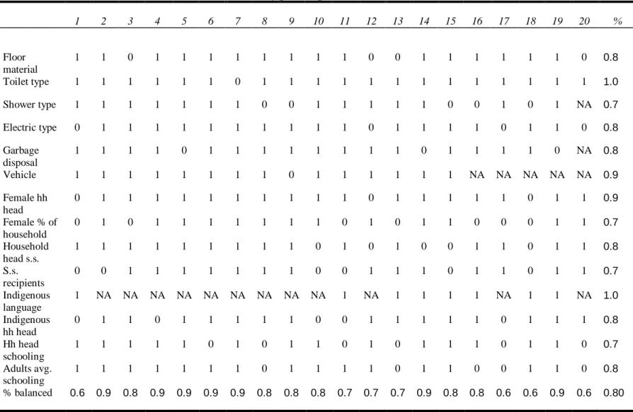
identical and suggest a statistically significant enrollment gain of about 0.05. Table IIB shows that with a few exceptions the matching procedure successfully selects matched pairs with very similar average baseline characteristics. Table IIc gives the breakdown of t-tests for each of 20 p-score quantiles and for all baseline covariates that are correlated with school enrollment. Results suggest that most variable-stratum cells (81 percent) are well balanced (i.e. produce insignificant t-tests at the 5% level) for most baseline characteristics. However, some covariates fail to balance in repeated strata, such as the percentage of social security recipients in the household. Table IIIa shows the results of a more flexible p-score specification (i.e. a probit equation that includes up to fifth-degree polynomials for some variables) which brings down the estimated ATT to about 0.04. With the exception of the adult social security recipients in the household and the propotion of household heads who only speak an indigenous language, the quintic model eliminates all average differences across baseline covariates (Table IIIb). Disaggregated balancing checks reveal that several baseline household characteristics remain unbalanced depending on the p-score stratum, and 80 percent of variable-stratum cells are balanced.
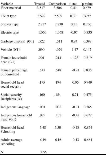
Table IVa reports results form the same quintic specification as above but excluding treatment observations which do not have a match within a 0.0001 p-score radius. This reduces the sample size by about 1500 households but impact estimates still lie between 0.04 and 0.05 and remain highly significant. The caliper restriction succeeds in balancing the remaining average difference in adult social security recipients and exclusive indigenous language prevalence. Table IVc shows that this specification also improves balance across variable-stratum cells. Overall, 87 percent of variable-stratum cells are balanced in terms of means. Adult average schooling remains unbalanced in several p-score strata, however.
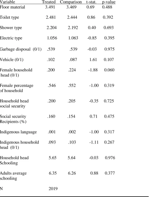
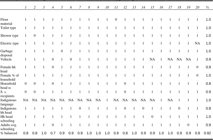
The final specification reported in table Va imposes an even closer match by dropping 2571 treated units that have no comparison units within a 0.00005 p-score radius from the estimation sample. ATT‘s are only slightly smaller in magnitude, around 0.04, and remain quite precisely estimated. Table Vc shows that balance now holds for all variables in at least 16 out of 20 p-score strata and for 92 percent of variable-stratum cells overall.
5. Conclusion
Another limitation of our analysis is that we have little to say about the effect of doubling the BDH benefits because we are comparing recipients to non-recipients, irrespective of when they entered the program. Put differently, we are unable to disentangle a medium term enrollment effect due to initial benefits from a short term enrollment effect due to the doubling of benefits in 2007. What we are estimating is the joint effect of the program‘s history, including the scaling up of benefits but excluding stricter enforcement of conditionality. One way to go about estimating the BDH effect inclusive of stricter conditionality would be to do a regression discontinuity analysis similar to Oosterbeek and Ponce based on the original Selben score but using the Selben survey as a data source for outcome measures for example (assuming that schooling is included). In order to isolate the pure effect of scaled up benefits cum conditionality under the new BDH regime we would need a new source of variation in BDH assignment, perhaps based on the updated Selben rosters, combined with another survey targeted at households around the new Selben cutoff a la Oosterbeek and Ponce.
6. References
Dehejia R. H. and S. Wahba, 2002, ―Propensity Score-Matching Methods for Nonexperimental Causal Studies‖, the Review of Economics and Statistics, 84(1), pp. 151-161
Oosterbeek, H. and Juan Ponce, 2007, ―The impact of unconditional cash transfers on school enrollment: Evidence from Ecuador‖, mimeo
Schady, N. and M. Araujo, 2006. ―Cash Transfers, Conditions and School Enrollment in Ecuador, Economia, forthcoming
T=0 T=1
Ti=1|S(Xi)
Non-complier
Tj=0|S(Xj)
Complier
.
Ts=1|S(Xs)
Complier
Tk=0|S(Xk)
Non-complier
Figure 1
Table I: Enrollment predictors
Dependent variable: Percent of 5-19 year olds enrolled in school
Coef. Std. Err. t P>t [95% Conf. Interval] House type -.0012167 .0026601 -0.46 0.647 -.0064311 .0039976 House owned -.0038107 .0030588 -1.25 0.213 -.0098064 .002185 Floor material -.0123659 .0029951 -4.13 0.000 -.0182367 -.006495 Toilet type -.0116635 .0033766 -3.45 0.001 -.0182823 -.0050447 Shower type -.0142807 .0039627 -3.60 0.000 -.0220482 -.0065132 Electric type -.0411027 .0149784 -2.74 0.006 -.0704628 -.0117427 Garbage disposal .0242649 .0088481 2.74 0.006 .0069212 .0416085 Rooms per capita -.0273402 .0136324 -2.01 0.045 -.054062 -.0006184 Bedrooms per capita -.0095541 .020759 -0.46 0.645 -.050245 .0311369 Vehicle .0204094 .0064312 3.17 0.002 .0078032 .0330157 Land owned .0006891 .0074804 0.09 0.927 -.0139737 .0153518 Land rented .0196452 .016831 1.17 0.243 -.0133462 .0526366 Female household head -.0855968 .0096713 -8.85 0.000 -.1045541 -.0666395 Female percentage .2742908 .019595 14.00 0.000 .2358814 .3127003 Elderly -.0050239 .010863 -0.46 0.644 -.026317 .0162693 Social security recipient .000052 .009489 0.01 0.996 -.018548 .018652 Social security recipients .0285863 .012832 2.23 0.026 .0034335 .0537392 Disabled -.0075138 .0156483 -0.48 0.631 -.0381869 .0231593 Indigenous language .0271617 .0572361 0.47 0.635 -.0850304 .1393537 Spanish & indig. Lang. .0097207 .017179 0.57 0.572 -.023953 .0433944 Indigenous .027014 .0158823 1.70 0.089 -.0041178 .0581458 Mulato .011457 .0125623 0.91 0.362 -.0131671 .0360812 HH head schooling .002712 .0011768 2.30 0.021 .0004053 .0050186 Adult average schooling .0099357 .0014942 6.65 0.000 .0070068 .0128646 N=11968
Table IIa (Quadratic Model)
Dependent variable: Percent of 5-19 year olds enrolled in school
Matching estimator OLS restricted to matched sample
ATT 0.049 0.049 SE 0.010 0.008
Notes: Single nearest neighbor propensity score matching with replacement. Propensity score model includes linear and quadratic terms of selected Selben variables. Comparison group observations are weighted by their matching frequency. OLS regression includes all covariates from the p-score equation in the outcome equation.
Table IIb (Quadratic Model): Mean differences in covariates
Variable Treated Comparison t-stat. p-value Floor material 3.601 3.570 1.43 0.153
Toilet type 2.651 2.640 0.37 0.709
Shower type 2.313 2.324 -0.56 0.572
Electric type 1.062 1.073 -1.88 0.061
Garbage disposal (0/1) .478 .4908 -1.21 0.226
Vehicle (0/1) .076 .0716 0.96 0.340
Female household .194 .213 -2.28 0.023 head (0/1)
Female percentage .547 .554 -1.65 0.100 of household
Household head .211 .181 3.55 0.000 social security
Social security .174 .145 4.45 0.000 Recipients (%)
Indigenous language .005 .006 -0.41 0.679
Indigenous household .126 .119 0.95 0.340 head (0/1)
Household head 5.22 5.18 0.52 0.605 Schooling
Adults average 5.93 5.95 -0.30 0.765 schooling
Table IIc (Quadratic Model): Mean differences in covariates by p-score quantile
1 2 3 4 5 6 7 8 9 10 11 12 13 14 15 16 17 18 19 20 %
Floor material 1 0 1 1 1 1 1 1 1 1 1 0 1 1 1 1 1 1 0 1 0.9
Toilet type 1 1 1 1 1 1 0 0 1 1 1 1 1 1 1 1 1 1 1 1 0.9
Shower type 1 1 1 1 1 1 1 1 1 1 1 0 0 0 1 1 1 0 0 1 0.8
Electric type 1 1 1 1 1 1 1 1 1 1 1 0 0 1 1 1 1 1 0 0 0.8
Garbage disposal
1 1 1 1 1 1 1 0 0 1 1 1 0 1 1 1 1 1 1 0 0.8
Vehicle 1 1 1 1 1 1 1 1 1 1 1 1 1 0 1 1 NA 1 NA NA 0.9
Female household head
1 1 1 1 1 1 1 1 0 1 1 1 1 0 1 1 1 1 1 1 0.9
Female % of household
1 1 1 1 1 1 0 1 1 1 1 1 1 1 1 1 1 1 1 1 1.0
Household head social security
0 1 1 1 1 1 1 1 1 0 1 1 1 1 0 0 0 1 0 1 0.7
Social security recipients
0 0 1 1 1 1 1 0 1 0 1 0 1 1 0 0 0 1 0 1 0.6
Indigenous language
1 1 0 1 1 1 0 1 1 1 1 1 1 1 0 1 0 1 1 1 0.8
Indigenous household head
1 1 0 0 1 1 0 1 1 1 1 1 1 1 0 1 0 1 1 1 0.8
Household head schooling
1 1 1 1 1 1 1 1 1 1 0 1 0 1 1 0 1 1 1 1 0.9
Adults average schooling
1 1 1 1 1 1 1 1 0 1 1 1 0 1 1 0 1 0 1 1 0.8
% balanced 0.9 0.9 0.9 0.9 1.0 1.0 0.7 0.8 0.8 0.9 0.9 0.7 0.6 0.8 0.7 0.7 0.7 0.9 0.6 0.8 0.81
Table IIIa (Quintic Model)
Dependent variable: Percent of 5-19 year olds enrolled in school
Matching estimator OLS restricted to matched sample
ATT 0.051 0.043 SE 0.010 0.008
Notes: Single nearest neighbor propensity score matching with replacement. Propensity score model includes linear and up to quintic terms of selected Selben variables. Comparison group observations are weighted by their matching frequency. OLS regression includes all covariates from the p-score equation in the outcome equation.
Table IIIb (Quintic Model): Mean differences in covariates
Variable Treated Comparison t-stat. p-value Floor material 3.601 3.607 -0.30 0.762
Toilet type 2.651 2.644 0.25 0.800
Shower type 2.313 2.332 -1.02 0.308
Electric type 1.062 1.056 -0.91 0.362
Garbage disposal (0/1) .478 .481 -0.31 0.754
Vehicle (0/1) .076 .0727 0.75 0.451
Female household .194 .189 -0.53 0.596 head (0/1)
Female percentage .547 .541 -1.57 0.116 of household
Household head .211 .194 1.95 0.052 social security
Social security .174 .159 2.27 0.023 Recipients (%)
Indigenous language .005 .001 2.75 0.006
Indigenous household .126 .117 1.28 0.202 head (0/1)
Household head 5.22 5.22 -0.11 0.913 Schooling
Adults average 5.93 5.89 -0.73 0.465 schooling
Table IIIc (Quintic Model): Mean differences in covariates by p-score quantile
1 2 3 4 5 6 7 8 9 10 11 12 13 14 15 16 17 18 19 20 %
Floor material
1 1 0 1 1 1 1 1 1 1 1 0 0 1 1 1 1 1 1 0 0.8
Toilet type 1 1 1 1 1 1 0 1 1 1 1 1 1 1 1 1 1 1 1 1 1.0
Shower type 1 1 1 1 1 1 1 0 0 1 1 1 1 1 0 0 1 0 1 NA 0.7
Electric type 0 1 1 1 1 1 1 1 1 1 1 0 1 1 1 1 0 1 1 0 0.8
Garbage disposal
1 1 1 1 0 1 1 1 1 1 1 1 1 0 1 1 1 1 0 NA 0.8
Vehicle 1 1 1 1 1 1 1 1 0 1 1 1 1 1 1 NA NA NA NA NA 0.9
Female hh head
0 1 1 1 1 1 1 1 1 1 1 0 1 1 1 1 1 0 1 1 0.9
Female % of household
0 1 0 1 1 1 1 1 1 1 0 1 0 1 1 0 0 0 1 1 0.7
Household head s.s.
1 1 1 1 1 1 1 1 1 0 1 0 1 0 0 1 1 0 1 1 0.8
S.s. recipients
0 0 1 1 1 1 1 1 1 0 0 1 1 1 0 1 1 0 1 1 0.7
Indigenous language
1 NA NA NA NA NA NA NA NA NA 1 NA 1 1 1 1 NA 1 1 NA 1.0
Indigenous hh head
0 1 1 0 1 1 1 1 1 0 0 1 1 1 1 1 0 1 1 1 0.8
Hh head schooling
1 1 1 1 1 0 1 0 1 1 0 1 0 1 1 1 0 1 1 0 0.7
Adults avg. schooling
1 1 1 1 1 1 1 0 1 1 1 1 0 1 1 0 0 1 1 0 0.8
% balanced 0.6 0.9 0.8 0.9 0.9 0.9 0.9 0.8 0.8 0.8 0.7 0.7 0.7 0.9 0.8 0.8 0.6 0.6 0.9 0.6 0.80
Table IVa (Quintic Model, caliper =0.0001)
Dependent variable: Percent of 5-19 year olds enrolled in school
Matching estimator OLS restricted to matched sample
ATT 0.047 0.042 SE 0.010 0.009
Notes: Single nearest neighbor propensity score matching with replacement.
Propensity score model includes linear and quintic terms of selected Selben variables. 1535 treated units that have no comparison units within a 0.0001 p-score radius are dropped from the sample. Comparison group observations are weighted by their matching frequency. OLS regression includes all covariates from the p-score equation in the outcome equation.
Table IVb (Quintic Model, caliper =0.0001): Mean differences in covariates
Variable Treated Comparison t-stat. p-value Floor material 3.517 3.506 0.41 0.679
Toilet type 2.522 2.509 0.39 0.699
Shower type 2.237 2.230 0.31 0.756
Electric type 1.060 1.068 -0.97 0.330
Garbage disposal (0/1) .522 .511 0.84 0.398
Vehicle (0/1) .090 .079 1.47 0.142
Female household .201 .214 -1.23 0.219 head (0/1)
Female percentage .547 .548 -0.21 0.836 of household
Household head .195 .194 0.06 0.949 social security
Social security .160 .154 0.71 0.475 Recipients (%)
Indigenous language .001 .002 -0.91 0.365
Indigenous household .099 .103 -0.42 0.672 head (0/1)
Household head 5.48 5.50 -0.18 0.854 Schooling
Table IVc (Quintic Model, caliper =0.0001): Mean differences in covariates by p-score quantile
1 2 3 4 5 6 7 8 9 10 11 12 13 14 15 16 17 18 19 20 %
Floor material
1 0 1 1 1 1 1 0 1 0 1 1 1 1 1 1 1 1 1 1 0.9
Toilet type 1 1 1 1 0 1 1 1 1 1 1 1 1 1 1 1 1 1 1 1 1.0
Shower type 1 0 1 1 0 1 1 1 1 1 1 1 0 1 1 1 1 0 1 1 0.8
Electric type 1 1 1 1 1 1 1 1 1 0 1 1 1 1 1 1 1 1 1 1 1.0
Garbage disposal
1 1 1 1 0 1 1 1 1 1 1 1 0 1 1 1 1 0 1 1 0.9
Vehicle 1 1 1 1 1 1 1 1 1 1 1 0 1 1 1 1 NA NA NA NA 0.9
Female hh head
1 1 1 0 0 1 1 1 1 1 1 1 1 1 1 1 0 1 1 1 0.9
Female % of household
1 1 1 0 1 1 1 1 1 0 1 1 1 1 1 1 1 1 1 1 0.9
Household head s.s.
0 0 0 1 1 1 1 1 1 1 1 1 1 1 1 1 1 1 0 0 0.8
S.s. recipients
0 0 1 1 1 1 0 1 1 1 0 1 1 1 1 1 1 1 1 0 0.8
Indigenous language
NA NA NA NA NA NA NA NA 1 NA NA NA NA NA 1 1 NA 1 1 1 1.0
Indigenous hh head
1 1 1 1 1 1 1 1 1 1 1 1 0 1 1 1 1 1 1 1 1.0
Hh head schooling
1 1 1 1 1 1 1 1 1 1 1 1 1 1 1 1 0 1 1 1 1.0
Adults avg. schooling
0 1 1 0 0 1 1 1 1 0 1 1 1 1 1 1 0 1 0 1 0.7
% balanced 0.8 0.7 0.9 0.8 0.6 1.0 0.9 0.9 1.0 0.7 0.9 0.9 0.8 1.0 1.0 1.0 0.8 0.8 0.8 0.8 0.87
Table Va: Percent of 5-19 year olds enrolled in school
Dependent variable: Percent of 5-19 year olds enrolled in school
Matching estimator OLS restricted to matched sample
ATT 0.037 0.040 SE 0.012 0.010
Notes: Single nearest neighbor propensity score matching with replacement. Propensity score model includes linear and quintic terms of selected Selben variables. 2571 treated units that have no comparison units within a 0.00005 p-score radius are dropped from the sample. Comparison group observations are weighted by their matching frequency. OLS regression includes all covariates from the p-score equation in the outcome equation.
Table Vb (Quintic Model, caliper =0.00005): Mean differences in covariates
Variable Treated Comparison t-stat. p-value Floor material 3.491 3.469 0.69 0.488
Toilet type 2.481 2.444 0.86 0.392
Shower type 2.204 2.192 0.40 0.693
Electric type 1.056 1.063 -0.85 0.395
Garbage disposal (0/1) .539 .539 -0.03 0.975
Vehicle (0/1) .102 .087 1.61 0.107
Female household .200 .224 -1.88 0.060 head (0/1)
Female percentage .546 .552 -1.00 0.319 of household
Household head .200 .205 -0.35 0.725 social security
Social security .160 .154 0.71 0.475 Recipients (%)
Indigenous language .001 .002 -1.00 0.317
Indigenous household .093 .103 -1.11 0.267 head (0/1)
Household head 5.65 5.64 -0.03 0.976 Schooling
Adults average 6.35 6.26 0.88 0.377 schooling
Table Vc (Quintic Model, caliper =0.00005): Mean differences in covariates by p-score quantile
1 2 3 4 5 6 7 8 9 10 11 12 13 14 15 16 17 18 19 20 %
Floor material
1 1 1 1 1 1 1 1 1 1 0 1 1 1 1 1 1 1 1 1 1.0
Toilet type 1 1 1 1 1 1 1 1 1 1 1 1 1 1 1 1 1 1 1 1 1.0
Shower type 1 0 1 1 1 1 1 1 1 1 1 1 1 1 1 1 1 1 1 1 1.0
Electric type 1 1 1 1 1 1 1 1 1 1 1 1 1 1 1 1 1 1 1 NA 1.0
Garbage disposal
1 1 1 1 0 1 1 1 1 1 1 1 1 1 1 1 1 1 1 1 1.0
Vehicle 1 1 1 0 1 0 1 1 1 1 1 1 1 1 NA 1 NA NA NA 1 0.9
Female hh head
1 1 1 0 1 1 1 1 1 1 1 1 1 1 1 1 1 1 1 0 0.9
Female % of household
1 1 1 1 1 1 1 1 1 1 1 1 1 1 1 1 1 1 1 0 1.0
Household head ss
0 0 1 0 1 1 1 1 1 1 1 0 1 1 1 1 1 1 1 1 0.8
S. s. recipients
0 0 1 1 1 1 1 1 1 1 1 0 1 1 1 1 1 1 1 1 0.9
Indigenous language
NA NA NA NA NA NA NA NA NA 1 NA NA NA NA NA 1 NA 1 1 1 1.0
Indigenous hh head
1 1 1 1 1 1 0 1 1 1 1 0 1 0 1 1 1 0 1 1 0.8
Hh head schooling
1 1 1 1 1 1 1 1 1 1 1 1 1 1 0 1 1 1 1 1 1.0
Adults avg. schooling
1 1 1 0 1 1 1 1 1 1 1 1 1 1 1 1 1 1 0 1 0.9
% balanced 0.8 0.8 1.0 0.7 0.9 0.9 0.9 1.0 1.0 1.0 0.9 0.8 1.0 0.9 0.9 1.0 1.0 0.9 0.9 0.8 0.92
Data Appendix
Variable
SIEH-ENEMDU Question Corresponding 2003 Selben Question Coding
House Type 1-1 1 1 – 6 descending scale
Ownership 1-2 2 1 – 3 descending scale
Floor Material 1-3 3 1 – 6 descending scale
Toilet type 1-7 4 1 – 5 descending scale
Shower type 1-9 5 1 – 3 descending scale
Electricity/Lighting 1-10 7 1 – 3 descending scale Garbage Disposal 1-11 8 1 if public or private service
Rooms per capita 1-4 9 Number of rooms per capita in house Bedrooms per
capita
1-5 10 Number of bedrooms per capita in
house
Vehicle 1-14 11 1 if household member owns a car or
motorcylce Own Land for
Agriculture
1-12 14/15 1 if household owns land for agricultural use
Rent/Share Land for Agriculture
1-13 14/15 1 if household rents land for agricultural use
Household Head Social Security
2-5 8 1 if household head has social
security (IESS, Military/Police, Private Insurance or Communal) Percent of Adults
with Social Security
2-5 8 Percent of adults in the household with social security
Disabled Adult 2-15D 9 1 if there is a disabled adult in the household
Elderly 2-3 1 if there is an adult over age 70 in
the household Indigenous
Language
2-14 10 1 if the household head speaks only an indigenous language
Indigenous and Spanish Language
2-14 10 1 if the household head speaks both Spanish and an indigenous language Indigenous Head 2-15 11 1 if household head describes
ethnicity as indigenous
Mulato Head 2-15 11 1 if household head describes
ethnicity as black or mulato Head Years of
Education
2-10 15 Household head‘s years of education Adults Years of
Education
2-10 15 Average number of years of