TE
AM
FL
Y
3D Math Primer for
Graphics and Game
Development
Fletcher Dunn
and Ian Parberry
Library of Congress Cataloging-in-Publication Data Dunn, Fletcher.
3D math primer for graphics and game development / by Fletcher Dunn and Ian Parberry. p. cm.
ISBN 1-55622-911-9
1. Computer graphics. 2. Computer games--Programming. 3. Computer science--Mathematics. I. Parberry, Ian. II. Title.
T385 .D875 2002
006.6--dc21 2002004615
CIP
© 2002, Wordware Publishing, Inc. All Rights Reserved 2320 Los Rios Boulevard
Plano, Texas 75074
No part of this book may be reproduced in any form or by any means without permission in writing from
Wordware Publishing, Inc.
Printed in the United States of America
ISBN 1-55622-911-9 10 9 8 7 6 5 4 3 2 1 0205
Product names mentioned are used for identification purposes only and may be trademarks of their respective companies.
All inquiries for volume purchases of this book should be addressed to Wordware Publishing, Inc., at the above address. Telephone inquiries may be made by calling:
Acknowledgments . . . xi
Chapter 1 Introduction . . . 1
1.1 What is 3D Math? . . . 1
1.2 Why You Should Read This Book . . . 1
1.3 What You Should Know Before Reading This Book . . . 3
1.4 Overview . . . 3
Chapter 2 The Cartesian Coordinate System . . . 5
2.1 1D Mathematics . . . 6
2.2 2D Cartesian Mathematics . . . 9
2.2.1 An Example: The Hypothetical City of Cartesia . . . 9
2.2.2 Arbitrary 2D Coordinate Spaces . . . 10
2.2.3 Specifying Locations in 2D Using Cartesian Coordinates . . . 13
2.3 From 2D to 3D . . . 14
2.3.1 Extra Dimension, Extra Axis . . . 15
2.3.2 Specifying Locations in 3D . . . 15
2.3.3 Left-handed vs. Right-handed Coordinate Spaces . . . 16
2.3.4 Some Important Conventions Used in This Book . . . 19
2.4 Exercises. . . 20
Chapter 3 Multiple Coordinate Spaces . . . 23
3.1 Why Multiple Coordinate Spaces? . . . 24
3.2 Some Useful Coordinate Spaces . . . 25
3.2.1 World Space . . . 25
3.2.2 Object Space . . . 26
3.2.3 Camera Space . . . 27
3.2.4 Inertial Space . . . 28
3.3 Nested Coordinate Spaces. . . 30
3.4 Specifying Coordinate Spaces . . . 31
3.5 Coordinate Space Transformations . . . 31
3.6 Exercises. . . 34
Chapter 4 Vectors . . . 35
4.1 Vector — A Mathematical Definition . . . 36
4.1.1 Vectors vs. Scalars . . . 36
4.1.2 Vector Dimension . . . 36
4.1.3 Notation . . . 36
4.2 Vector — A Geometric Definition . . . 37
4.2.1 What Does a Vector Look Like? . . . 37
4.2.2 Position vs. Displacement . . . 38
4.2.3 Specifying Vectors . . . 38
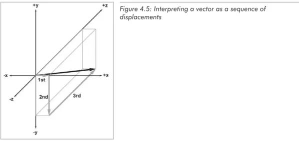
4.2.4 Vectors as a Sequence of Displacements . . . 39
4.3 Vectors vs. Points . . . 40
4.3.1 Relative Position . . . 41
4.3.2 The Relationship Between Points and Vectors . . . 41
4.4 Exercises. . . 42
Chapter 5 Operations on Vectors . . . 45
5.1 Linear Algebra vs. What We Need . . . 46
5.2 Typeface Conventions . . . 46
5.3 The Zero Vector . . . 47
5.4 Negating a Vector . . . 48
5.4.1 Official Linear Algebra Rules . . . 48
5.4.2 Geometric Interpretation . . . 48
5.5 Vector Magnitude (Length) . . . 49
5.5.1 Official Linear Algebra Rules . . . 49
5.5.2 Geometric Interpretation . . . 50
5.6 Vector Multiplication by a Scalar . . . 51
5.6.1 Official Linear Algebra Rules . . . 51
5.6.2 Geometric Interpretation . . . 52
5.7 Normalized Vectors . . . 53
5.7.1 Official Linear Algebra Rules . . . 53
5.7.2 Geometric Interpretation . . . 53
5.8 Vector Addition and Subtraction . . . 54
5.8.1 Official Linear Algebra Rules . . . 54
5.8.2 Geometric Interpretation . . . 55
5.8.3 Vector from One Point to Another . . . 57
5.9 The Distance Formula . . . 57
5.10 Vector Dot Product . . . 58
5.10.1 Official Linear Algebra Rules . . . 58
5.10.2 Geometric Interpretation . . . 59
5.10.3 Projecting One Vector onto Another . . . 61
5.11 Vector Cross Product. . . 62
5.11.1 Official Linear Algebra Rules . . . 62
5.11.2 Geometric Interpretation . . . 62
5.12 Linear Algebra Identities . . . 65
5.13 Exercises . . . 67
Chapter 6 A Simple 3D Vector Class . . . 69
6.1 Class Interface . . . 69
6.2 Class Vector3 Definition . . . 70
6.3 Design Decisions . . . 73
6.3.1 Floats vs. Doubles . . . 73
6.3.2 Operator Overloading . . . 73
iv
6.3.3 Provide Only the Most Important Operations . . . 74
6.3.4 Don’t Overload Too Many Operators . . . 74
6.3.5 Use Const Member Functions . . . 75
6.3.6 Use Const & Arguments . . . 75
6.3.7 Member vs. Nonmember Functions . . . 75
6.3.8 No Default Initialization . . . 77
6.3.9 Don’t Use Virtual Functions . . . 77
6.3.10 Don’t Use Information Hiding . . . 77
6.3.11 Global Zero Vector Constant . . . 78
6.3.12 No “point3” Class. . . 78
6.3.13 A Word on Optimization . . . 78
Chapter 7 Introduction to Matrices . . . 83
7.1 Matrix — A Mathematical Definition . . . 83
7.1.1 Matrix Dimensions and Notation . . . 83
7.1.2 Square Matrices . . . 84
7.1.3 Vectors as Matrices. . . 85
7.1.4 Transposition . . . 85
7.1.5 Multiplying a Matrix with a Scalar . . . 86
7.1.6 Multiplying Two Matrices . . . 86
7.1.7 Multiplying a Vector and a Matrix. . . 89
7.1.8 Row vs. Column Vectors . . . 90
7.2 Matrix — A Geometric Interpretation . . . 91
7.2.1 How Does a Matrix Transform Vectors? . . . 92
7.2.2 What Does a Matrix Look Like?. . . 93
7.2.3 Summary . . . 97
7.3 Exercises. . . 98
Chapter 8 Matrices and Linear Transformations . . . 101
8.1 Transforming an Object vs. Transforming the Coordinate Space . . . 102
8.2 Rotation . . . 105
8.2.1 Rotation in 2D . . . 105
8.2.2 3D Rotation about Cardinal Axes . . . 106
8.2.3 3D Rotation about an Arbitrary Axis. . . 109
8.3 Scale . . . 112
8.3.1 Scaling along Cardinal Axes . . . 112
8.3.2 Scale in an Arbitrary Direction . . . 113
8.4 Orthographic Projection . . . 115
8.4.1 Projecting onto a Cardinal Axis or Plane. . . 116
8.4.2 Projecting onto an Arbitrary Line or Plane. . . 117
8.5 Reflection . . . 117
8.6 Shearing . . . 118
8.7 Combining Transformations . . . 119
8.8 Classes of Transformations . . . 120
8.8.1 Linear Transformations . . . 121
8.8.2 Affine Transformations . . . 122
8.8.3 Invertible Transformations . . . 122
8.8.4 Angle-preserving Transformations . . . 122
8.8.5 Orthogonal Transformations . . . 122
8.8.6 Rigid Body Transformations . . . 123
8.8.7 Summary of Types of Transformations . . . 123
8.9 Exercises . . . 124
Chapter 9 More on Matrices . . . 125
9.1 Determinant of a Matrix . . . 125
9.1.1 Official Linear Algebra Rules . . . 125
9.1.2 Geometric Interpretation . . . 129
9.2 Inverse of a Matrix . . . 130
9.2.1 Official Linear Algebra Rules . . . 130
9.2.2 Geometric Interpretation . . . 132
9.3 Orthogonal Matrices . . . 132
9.3.1 Official Linear Algebra Rules . . . 132
9.3.2 Geometric Interpretation . . . 133
9.3.3 Orthogonalizing a Matrix . . . 134
9.4 4×4 Homogenous Matrices . . . 135
9.4.1 4D Homogenous Space . . . 136
9.4.2 4×4 Translation Matrices . . . 137
9.4.3 General Affine Transformations . . . 140
9.4.4 Perspective Projection . . . 141
9.4.5 A Pinhole Camera. . . 142
9.4.6 Perspective Projection Using 4×4 Matrices . . . 145
9.5 Exercises . . . 146
Chapter 10 Orientation and Angular Displacement in 3D . . . . 147
10.1 What is Orientation? . . . 148
10.2 Matrix Form . . . 149
10.2.1 Which Matrix? . . . 150
10.2.2 Advantages of Matrix Form . . . 150
10.2.3 Disadvantages of Matrix Form . . . 151
10.2.4 Summary . . . 152
10.3 Euler Angles . . . 153
10.3.1 What are Euler Angles? . . . 153
10.3.2 Other Euler Angle Conventions . . . 155
10.3.3 Advantages of Euler Angles. . . 156
10.3.4 Disadvantages of Euler Angles . . . 156
10.3.5 Summary . . . 159
10.4 Quaternions . . . 159
10.4.1 Quaternion Notation . . . 160
10.4.2 Quaternions as Complex Numbers . . . 160
10.4.3 Quaternions as an Axis-Angle Pair . . . 162
10.4.4 Quaternion Negation . . . 163
10.4.5 Identity Quaternion(s) . . . 163
vi
10.4.6 Quaternion Magnitude. . . 163
10.4.7 Quaternion Conjugate and Inverse . . . 164
10.4.8 Quaternion Multiplication (Cross Product) . . . 165
10.4.9 Quaternion “Difference” . . . 168
10.4.10 Quaternion Dot Product . . . 169
10.4.11 Quaternion Log, Exp, and Multiplication by a Scalar. . . 169
10.4.12 Quaternion Exponentiation . . . 171
10.4.13 Quaternion Interpolation — aka “Slerp” . . . 173
10.4.14 Quaternion Splines — aka “Squad” . . . 177
10.4.15 Advantages/Disadvantages of Quaternions . . . 178
10.5 Comparison of Methods . . . 179
10.6 Converting between Representations . . . 180
10.6.1 Converting Euler Angles to a Matrix . . . 180
10.6.2 Converting a Matrix to Euler Angles . . . 182
10.6.3 Converting a Quaternion to a Matrix . . . 185
10.6.4 Converting a Matrix to a Quaternion . . . 187
10.6.5 Converting Euler Angles to a Quaternion . . . 190
10.6.6 Converting a Quaternion to Euler Angles . . . 191
10.7 Exercises . . . 193
Chapter 11 Transformations in C++ . . . 195
11.1 Overview . . . 196
11.2 Class EulerAngles . . . 198
11.3 Class Quaternion . . . 205
11.4 Class RotationMatrix . . . 215
11.5 Class Matrix4×3 . . . 220
Chapter 12 Geometric Primitives . . . 239
12.1 Representation Techniques . . . 239
12.1.1 Implicit Form . . . 239
12.1.2 Parametric Form . . . 240
12.1.3 “Straightforward” Forms . . . 240
12.1.4 Degrees of Freedom . . . 241
12.2 Lines and Rays . . . 241
12.2.1 Two Points Representation . . . 242
12.2.2 Parametric Representation of Rays . . . 242
12.2.3 Special 2D Representations of Lines . . . 243
12.2.4 Converting between Representations . . . 245
12.3 Spheres and Circles . . . 246
12.4 Bounding Boxes . . . 247
12.4.1 Representing AABBs . . . 248
12.4.2 Computing AABBs . . . 249
12.4.3 AABBs vs. Bounding Spheres . . . 250
12.4.4 Transforming AABBs . . . 251
12.5 Planes . . . 252
12.5.1 Implicit Definition — The Plane Equation . . . 252
12.5.2 Definition Using Three Points . . . 253
12.5.3 “Best-fit” Plane for More Than Three Points . . . 254
12.5.4 Distance from Point to Plane . . . 256
12.6 Triangles . . . 257
12.6.1 Basic Properties of a Triangle . . . 257
12.6.2 Area of a Triangle . . . 258
12.6.3 Barycentric Space . . . 260
12.6.4 Special Points . . . 267
12.7 Polygons . . . 269
12.7.1 Simple vs. Complex Polygons . . . 269
12.7.2 Self-intersecting Polygons . . . 270
12.7.3 Convex vs. Concave Polygons . . . 271
12.7.4 Triangulation and Fanning . . . 274
12.8 Exercises . . . 275
Chapter 13 Geometric Tests . . . 277
13.1 Closest Point on 2D Implicit Line . . . 277
13.2 Closest Point on Parametric Ray . . . 278
13.3 Closest Point on Plane . . . 279
13.4 Closest Point on Circle/Sphere . . . 280
13.5 Closest Point in AABB . . . 280
13.6 Intersection Tests . . . 281
13.7 Intersection of Two Implicit Lines in 2D . . . 282
13.8 Intersection of Two Rays in 3D . . . 283
13.9 Intersection of Ray and Plane . . . 284
13.10 Intersection of AABB and Plane . . . 285
13.11 Intersection of Three Planes . . . 286
13.12 Intersection of Ray and Circle/Sphere . . . 286
13.13 Intersection of Two Circles/Spheres . . . 288
13.14 Intersection of Sphere and AABB . . . 291
13.15 Intersection of Sphere and Plane . . . 291
13.16 Intersection of Ray and Triangle . . . 293
13.17 Intersection of Ray and AABB . . . 297
13.18 Intersection of Two AABBs . . . 297
13.19 Other Tests. . . 299
13.20 Class AABB3 . . . 300
13.21 Exercises. . . 316
Chapter 14 Triangle Meshes . . . 319
14.1 Representing Meshes . . . 320
14.1.1 Indexed Triangle Mesh . . . 320
14.1.2 Advanced Techniques . . . 322
14.1.3 Specialized Representations for Rendering . . . 322
14.1.4 Vertex Caching . . . 323
14.1.5 Triangle Strips . . . 323
14.1.6 Triangle Fans . . . 327
viii
14.2 Additional Mesh Information . . . 328
14.2.1 Texture Mapping Coordinates. . . 328
14.2.2 Surface Normals . . . 328
14.2.3 Lighting Values . . . 330
14.3 Topology and Consistency . . . 330
14.4 Triangle Mesh Operations . . . 331
14.4.1 Piecewise Operations . . . 331
14.4.2 Welding Vertices. . . 331
14.4.3 Detaching Faces . . . 334
14.4.4 Edge Collapse . . . 335
14.4.5 Mesh Decimation . . . 335
14.5 A C++ Triangle Mesh Class . . . 336
Chapter 15 3D Math for Graphics . . . 345
15.1 Graphics Pipeline Overview . . . 346
15.2 Setting the View Parameters . . . 349
15.2.1 Specifying the Output Window . . . 349
15.2.2 Pixel Aspect Ratio . . . 350
15.2.3 The View Frustum . . . 351
15.2.4 Field of View and Zoom. . . 351
15.3 Coordinate Spaces . . . 354
15.3.1 Modeling and World Space . . . 354
15.3.2 Camera Space . . . 354
15.3.3 Clip Space . . . 355
15.3.4 Screen Space . . . 357
15.4 Lighting and Fog . . . 358
15.4.1 Math on Colors . . . 359
15.4.2 Light Sources . . . 360
15.4.3 The Standard Lighting Equation — Overview . . . 361
15.4.4 The Specular Component . . . 362
15.4.5 The Diffuse Component . . . 365
15.4.6 The Ambient Component . . . 366
15.4.7 Light Attenuation . . . 366
15.4.8 The Lighting Equation — Putting It All Together . . . 367
15.4.9 Fog . . . 368
15.4.10 Flat Shading and Gouraud Shading . . . 370
15.5 Buffers . . . 372
15.6 Texture Mapping . . . 373
15.7 Geometry Generation/Delivery . . . 374
15.7.1 LOD Selection and Procedural Modeling. . . 375
15.7.2 Delivery of Geometry to the API . . . 375
15.8 Transformation and Lighting . . . 377
15.8.1 Transformation to Clip Space . . . 378
15.8.2 Vertex Lighting . . . 378
15.9 Backface Culling and Clipping. . . 380
15.9.1 Backface Culling . . . 380
15.9.2 Clipping . . . 381
15.10 Rasterization. . . 383
Chapter 16 Visibility Determination . . . 385
16.1 Bounding Volume Tests . . . 386
16.1.1 Testing Against the View Frustum . . . 387
16.1.2 Testing for Occlusion . . . 390
16.2 Space Partitioning Techniques . . . 390
16.3 Grid Systems . . . 392
16.4 Quadtrees and Octrees . . . 393
16.5 BSP Trees . . . 398
16.5.1 “Old School” BSPs . . . 400
16.5.2 Arbitrary Dividing Planes . . . 401
16.6 Occlusion Culling Techniques . . . 402
16.6.1 Potentially Visible Sets . . . 402
16.6.2 Portal Techniques . . . 403
Chapter 17 Afterword . . . 407
Appendix A Math Review. . . 409
Summation Notation . . . 409
Angles, Degrees, and Radians . . . 409
Trig Functions . . . 410
Trig Identities . . . 413
Appendix B References . . . 415
Index . . . 417
x
Contents
TE
AM
FL
Y
Fletcher would like to thank his high school senior English teacher. She provided constant encour-agement and help with proofreading, even though she wasn’t really interested in 3D math. She is also his mom. Fletcher would also like to thank his dad for calling him every day to check on the progress of the book or just to talk. Fletcher would like to thank his boss, Mark Randel, for being an excellent teacher, mentor, and role model. Thanks goes to Chris DeSimone and Mario Merino as well, who (unlike Fletcher) actually have artistic ability and helped out with some of the more tricky diagrams in 3D Studio Max. A special thanks to Allen Bogue, Jeff Mills, Jeff Wilkerson, Matt Bogue, Todd Poynter, and Nathan Peugh for their opinions and feedback.
Ian would like to thank his wife for not threatening to cause him physical harm when he took mul-tiple weekends away from his family duties to work on this book. He would like to thank his children for not whiningtoo loudly. Also, thanks to the students of his Advanced Game Pro-gramming class at the University of North Texas in Spring 2002 for commenting on parts of this book in class. Oh, and thanks to Keith Smiley for the dead sheep.
Both authors would like to extend a very special thanks to Jim and Wes at Wordware for being very patient and providingmultipleextensions when it was inconvenient for them to do so.
Introduction
1.1 What is 3D Math?
This book is about 3D math, the study of the mathematics behind the geometry of a 3D world. 3D math is related to computational geometry, which deals with solving geometric problems algorith-mically. 3D math and computational geometry have applications in a wide variety of fields that use computers to model or reason about the world in 3D, such as graphics, games, simulation, robotics, virtual reality, and cinematography.
This book covers theory and practice in C++. The “theory” part is an explanation of the rela-tionship between math and geometry in 3D. It also serves as a handy reference for techniques and equations. The “practice” part illustrates how these concepts can be applied in code. The program-ming language used is C++, but in principle, the theoretical techniques from this book can be applied in any programming language.
This bookis notjust about computer graphics, simulation, or even computational geometry. However, if you plan to study those subjects, you will definitely need the information in this book.
1.2 Why You Should Read This Book
If you want to learn about 3D math in order to program games or graphics, then this book is for you. There are many books out there that promise to teach you how to make a game or put cool pictures up on the screen, so why should you readthisparticular book? This book offers several unique advantages over other books about games or graphics programming:
n A unique topic. This book fills a gap that has been left by other books on graphics, linear algebra, simulation, and programming. It is anintroductorybook, meaning we have focused our efforts on providing thorough coverage on fundamental 3D concepts — topics that are normally glossed over in a few quick pages or relegated to an appendix in other publications (because, after all, you already know all this stuff). Our book is definitely the book you should readfirst, before buying that “Write a 3D Video Game in 21 Days” book. This book is not only an introductory book, it is also a reference book — a “toolbox” of equations and techniques that you can browse through on a first reading and then revisit when the need for a specific tool arises.
n A unique approach. We take a three-pronged approach to the subject matter:math, geome-try, andcode. Themathpart is the equations and numbers. This is where most books stop. Of course, the math is important, but to make it powerful, you have to have good intuition about how the math connects with thegeometry. We will show you not just one butmultipleways to relate the numbers with the geometry on a variety of subjects, such as orientation in 3D, matrix multiplication, and quaternions. After the intuition comes the implementation; the codepart is the practical part. We show real usable code that makes programming 3D math as easy as possible.
n Unique authors. Our combined experience brings together academic authority with in-the-trenches practical advice. Fletcher Dunn has six years of professional game program-ming experience and several titles under his belt on a variety of gaprogram-ming platforms. He is cur-rently employed as the principal programmer at Terminal Reality and is the lead programmer onBloodRayne. Dr. Ian Parberry has 18 years of experience in research and teaching in acade-mia. This is his sixth book, his third on game programming. He is currently a tenured full pro-fessor in the Department of Computer Sciences at the University of North Texas. He is nationally known as one of the pioneers of game programming in higher education and has been teaching game programming to undergraduates at the University of North Texas since 1993.
n Unique pictures. You cannot learn about a subject like 3D by just reading text or looking at equations. You need pictures, and this book has plenty of them. Flipping through, you will notice that in many sections there is one on almost every page. In other words, we don’t just tellyou something about 3D math, weshowyou. You’ll also notice that pictures often appear beside equations or code. Again, this is a result of our unique approach that combines mathe-matical theory, geometric intuition, and practical implementation.
n Unique code. Unlike the code in some other books, the classes in this book are not designed to provide every possible operation you could ever want. Theyaredesigned to perform spe-cific functions very well and to be easy to understand and difficult to misuse. Because of their simple and focused semantics, you can write a line of code and have it work thefirsttime, without twiddling minus signs, swapping sines and cosines, transposing matrices, or other-wise employing “random engineering” until it looks right. Many other books exhibit a com-mon class design flaw of providingeverypossible operation when only a few are actually useful.
n A unique writing style. Our style is informal and entertaining, but formal and precise when clarity is important. Our goal is not to amuse you with unrelated anecdotes, but to engage you with interesting examples.
n A unique web page. This book does not come with a CD. CDs are expensive and cannot be updated once they are released. Instead, we have created a companion web page,
gamemath.com. There you will be able to experience interactive demos of some of the con-cepts that are the hardest to grasp from text and diagrams. You can also download the code (including any bug fixes!) and other useful utilities, find the answers to the exercises, and check out links to other sites concerning 3D math, graphics, and programming.
1.3 What You Should Know Before Reading
This Book
Thetheorypart of this book assumes a prior knowledge of basic algebra and geometry, such as:
n Manipulating algebraic expressions
n Algebraic laws, such as the associative and distributive laws
n Functions and variables
n Basic 2D Euclidian geometry
In addition, some prior exposure to trigonometry is useful, but not required. A brief review of some key mathematical concepts is included in Appendix A.
For thepracticepart, you need to understand some basics of programming in C++:
n Program flow control constructs
n Functions and parameters
n Object-oriented programming and class design
No specific compiler or target platform is assumed. No “advanced” C++ language features are used. The few language features that you may be unfamiliar with, such as operator overloading and reference arguments, will be explained as they are needed.
1.4 Overview
n Chapter 1 is the introduction, which you have almost finished reading. Hopefully, it has explained for whom this book is written and why we think you should read the rest of it.
n Chapter 2explains the Cartesian coordinate system in 2D and 3D and discusses how the Car-tesian coordinate system is used to locate points in space.
n Chapter 3discusses examples of coordinate spaces and how they are nested in a hierarchy.
n Chapter 4introduces vectors and explains the geometric and mathematical interpretations of vectors.
n Chapter 5discusses mathematical operations on vectors and explains the geometric interpre-tation of each operation.
n Chapter 6provides a usable C++ 3D vector class.
n Chapter 7 introduces matrices from a mathematical and geometric perspective and shows how matrices can be used to perform linear transformations.
n Chapter 8discusses different types of linear transformations and their corresponding matri-ces in detail.
n Chapter 9covers a few more interesting and useful properties of matrices.
n Chapter 11provides C++ classes for performing the math from Chapters 7 to 10.
n Chapter 12introduces a number of geometric primitives and discusses how to represent and manipulate them mathematically.
n Chapter 13 presents an assortment of useful tests that can be performed on geometric primitives.
n Chapter 14discusses how to store and manipulate triangle meshes and presents a C++ class designed to hold triangle meshes.
n Chapter 15is a survey of computer graphics with special emphasis on key mathematical points.
n Chapter 16discusses a number of techniques for visibility determination, an important issue in computer graphics.
n Chapter 17 reminds you to visit our web page and gives some suggestions for further reading.
The Cartesian
The Cartesian
Coordinate System
Coordinate System
3D math is all about measuring locations, distances, and angles precisely and mathematically in 3D space. The most frequently used framework to perform such measurements is called the Carte-sian coordinate system. Cartesian mathematics was invented by, and named after, a brilliant French philosopher, physicist, physiologist, and mathematician named René Descartes who lived
5
This chapter describes the basic concepts of 3D math. It is divided into three main sections.
n Section 2.1 is about 1D mathematics, the mathematics of counting and measuring. The main concepts introduced are:
u The math concepts of natural numbers, integers, rational numbers, and real numbers.
u The relationship between the naturals, integers, rationals and reals on one hand and the programming language concepts ofshort,int,float, anddoubleon the other hand.
u The First Law of Computer Graphics.
n Section 2.2 introduces 2D Cartesian mathematics, the mathematics of flat surfaces. The main concepts introduced are:
u The 2D Cartesian plane
u The origin
u Thex- andy-axes
u Orienting the axes in 2D
u Locating a point in 2D space using Cartesian (x,y) coordinates
n Section 2.3 extends 2D Cartesian math into 3D. The main concepts introduced are:
u Thez-axis
u Thexy,xz, andyzplanes
u Locating a point in 3D space using Cartesian (x,y,z) coordinates
from 1596 to 1650. Descartes is not just famous for inventing Cartesian mathematics, which at the time was a stunning unification of algebra and geometry. He is also well known for taking a pretty good stab at answering the question “How do I know something is true?” This question has kept generations of philosophers happily employed and does not necessarily involve dead sheep (which will disturbingly be a central feature of the next section), unless you really want it to. Des-cartes rejected the answers proposed by the ancient Greeks, which areethos(roughly, “because I told you so”),pathos(“because it would be nice”), andlogos(“because it makes sense”), and set about figuring it out for himself with a pencil and paper.
2.1 1D Mathematics
You’re reading this book because you want to know about 3D mathematics, so you’re probably wondering why we’re bothering to talk about 1D math. Well, there are a couple of issues about number systems and counting that we would like to clear up before we get to 3D.
Natural numbers, often calledcounting numbers, were invented millennia ago, probably to keep track of dead sheep. The concept of “one sheep” came easily (see Figure 2.1), then “two sheep” and “three sheep,” but people very quickly became convinced that this was too much work. They gave up counting at some point and invariably began using “many sheep.” Different cultures gave up at different points, depending on their threshold of boredom. Eventually, civilization expanded to the point where we could afford to have people sitting around thinking about numbers instead of doing more survival-oriented tasks, such as killing sheep and eating them. These savvy thinkers immortalized the concept of zero (no sheep), and while they didn’t get around to namingallof the natural numbers, they figured out various systems whereby we couldname them if we really wanted to, using digits such as “1”, “2”, etc. (or if you were Roman, “M”, “X”, “I,” etc.). Mathe-matics was born.
6
Chapter 2: The Cartesian Coordinate SystemFigure 2.1: One dead sheep
The habit of lining sheep up in a row so that they can easily be counted leads to the concept of anumber line, that is, a line with the numbers marked off at regular intervals, as in Figure 2.2. This line can, in principle, go on for as long as we wish, but to avoid boredom we have stopped at five sheep and put on an arrowhead to let you know that the line can continue. Clear thinkers can visu-alize it going off to infinity, but historical purveyors of dead sheep probably gave this concept little thought, outside of their dreams and fevered imaginings.
At some point in history it was probably realized that you can sometimes, if you are a particu-larly fast talker, sell a sheep that you don’t actually own, thus, simultaneously inventing the important concepts ofdebtandnegative numbers. Having sold this putative sheep, you would in fact own “negative one” sheep. This would lead to the discovery ofintegers, which consist of the natural numbers and their negative counterparts. The corresponding number line for integers is shown in Figure 2.3.
The concept of poverty probably predated that of debt, leading to a growing number of people who could afford to purchase only half a dead sheep, or perhaps only a quarter. This lead to a burgeon-ing use of fractional numbers, consistburgeon-ing of one integer divided by another, such as 2/3 or 111/27. Mathematicians called these rational numbers, and they fit in the number line in the obvious places between the integers. At some point, people became lazy and invented decimal notation, like writing “3.1415” instead of the longer and more tedious 31415/10000.
After a while, it was noticed that some numbers that appear to turn up in everyday life are not expressible as rational numbers. The classic example is the ratio of the circumference of a circle to its diameter, usually denoted asp (pronounced “pi”). These are the so-calledreal numbers, which include rational numbers and numbers such asp that would, if expressed in decimal form, require an infinite number of decimal places. The mathematics of real numbers is regarded by many to be the most important area of mathematics, and since it is the basis for most forms of engineering, it can be credited with creating much of modern civilization. The cool thing about real numbers is that while rational numbers are countable (that is, placed into one-to-one correspondence with the natural numbers), real numbers are uncountable. The study of natural numbers and integers is calleddiscrete mathematics, and the study of real numbers is calledcontinuous mathematics.
The truth is, however, that real numbers are nothing more than a polite fiction. They are a rela-tively harmless delusion, as any reputable physicist will tell you. The universe seems to be not only discrete, but also finite. If there are a finite amount of discrete things in the universe, as cur-rently appears to be the case, then it follows that we can only count to a certain fixed number. Thereafter, we run out of things to count — not only do we run out of dead sheep, but toasters, mechanics, and telephone sanitizers also. It follows that we can describe the universe using only
discrete mathematics, and requiring the use of only a finite subset of the natural numbers at that. (Large, yes, but finite.) Somewhere there may be an alien civilization with a level of technology exceeding ours that has never heard of continuous mathematics, the Fundamental Theorem of Calculus, or even the concept of infinity; even if we persist, they will firmly but politely insist on having no truck withp , being perfectly happy to build toasters, bridges, skyscrapers, mass transit, and starships using 3.14159 (or perhaps 3.1415926535897932384626433832795, if they are fas-tidious) instead.
So why do we use continuous mathematics? It is a useful tool that allows us to do engineering, but the real world is, despite the cognitive dissonance involved in using the term “real,” discrete. How does that affect you, the designer of a 3D computer-generated virtual reality? The computer is by its very nature discrete and finite, and you are more likely to run into the consequences of the discreteness and finiteness during its creation that you are likely to in the real world. C++ gives you a variety of different number forms that you can use for counting or measuring in your virtual world. These are theshort, theint, thefloatand thedouble, which can be described as follows (assuming the current PC technology). Theshortis a 16-bit integer that can store 65,536 different values, which means that “many sheep” for a 16-bit computer is 65,537. This sounds like a lot of sheep, but it isn’t adequate for measuring distances inside any reasonable kind of virtual reality that take people more than a few minutes to explore. Theintis a 32-bit integer that can store up to 4,294,967,296 different values, which is probably enough for your purposes. Thefloatis a 32-bit value that can store a subset of the rationals — 4,294,967,296 of them, the details not being impor-tant here. The double is similar, though using 64 bits instead of 32. We will return to this discussion in Section 6.3.1.
The bottom line in choosing to count and measure in your virtual world usingints,floats, or doubles is not, as some misguided people would have it, a matter of choosing between discrete shorts andints versus continuousfloats anddoubles. It is more a matter of precision. They are all discrete in the end. Older books on computer graphics will advise you to use integers because floating-point hardware is slower than integer hardware, but this is no longer the case. So which should you choose? At this point, it is probably best to introduce you to the First Law of Computer Graphics and leave you to think about it:
The First Law of Computer Graphics: If it looks right, itisright.
We will be doing a large amount of trigonometry in this book. Trigonometry involves real numbers, such asp , and real-valued functions, such as sine and cosine (which we’ll get to later). Real numbers are a convenient fiction, so we will continue to use them. How do you know this is true? You know because, Descartes notwithstanding, we told you so, because it would be nice, and because it makes sense.
8
Chapter 2: The Cartesian Coordinate SystemTE
AM
FL
Y
2.2 2D Cartesian Mathematics
You have probably used 2D Cartesian coordinate systems even if you have never heard the term Cartesianbefore.Cartesianis mostly just a fancy word for rectangular. If you have ever looked at the floor plans of a house, used a street map, seen a football game, or played chess, you have been exposed to 2D Cartesian coordinate space.
2.2.1 An Example: The Hypothetical City of Cartesia
Let’s imagine a fictional city named Cartesia. When the Cartesia city planners were laying out the streets, they were very particular, as illustrated in the map of Cartesia in Figure 2.4.
As you can see from the map, Center Street runs east-west through the middle of town. All other east-west streets (parallel to Center Street) are named based on whether they are north or south of Center Street and how far away they are from Center Street. Examples of streets which run east-west are North 3rd Street and South 15th Street.
The other streets in Cartesia run north-south. Division Street runs north-south through the middle of town. All other north-south streets (parallel to Division Street) are named based on whether they are east or west of Division street, and how far away they are from Division Street. So we have streets such as East 5th Street and West 22nd Street.
The naming convention used by the city planners of Cartesia may not be creative, but it cer-tainly is practical. Even without looking at the map, it is easy to find the doughnut shop at North 4th and West 2nd. It’s also easy to determine how far you will have to drive when traveling from one place to another. For example, to go from that doughtnut shop at North 4th and West 2nd to the police station at South 3rd and Division, you would travel seven blocks south and two blocks east.
2.2.2 Arbitrary 2D Coordinate Spaces
Before Cartesia was built, there was nothing but a large flat area of land. The city planners arbi-trarily decided where the center of town would be, which direction to make the roads run, how far apart to space the roads, etc. Much like the Cartesia city planners laid down the city streets, we can establish a 2D Cartesian coordinate system anywhere we want — on a piece of paper, a chess-board, a chalkchess-board, a slab of concrete, or a football field.
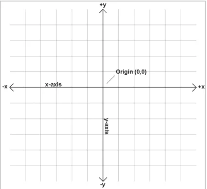
Figure 2.5 shows a diagram of a 2D Cartesian coordinate system.
10
Chapter 2: The Cartesian Coordinate SystemAs illustrated in Figure 2.5, a 2D Cartesian coordinate space is defined by two pieces of information:
n Every 2D Cartesian coordinate space has a special location, called theorigin, which is the “center” of the coordinate system. The origin is analogous to the center of the city in Cartesia.
n Every 2D Cartesian coordinate space has two straight lines that pass through the origin. Each line is known as anaxisand extends infinitely in two opposite directions. The two axes are perpendicular to each other. (Actually, they don’thaveto be, but most of the coordinate sys-tems we will look at will have perpendicular axes.) The two axes are analogous to Center and Division streets in Cartesia. The grid lines in the diagram are analogous to the other streets in Cartesia.
At this point, it is important to highlight a few significant differences between Cartesia and an abstract mathematical 2D space:
n The city of Cartesia has official city limits. Land outside of the city limits is not considered part of Cartesia. A 2D coordinate space, however, extends infinitely. Even though we usually only concern ourselves with a small area within the plane defined by the coordinate space, this plane, in theory, is boundless. In addition, the roads in Cartesia only go a certain distance (per-haps to the city limits), and then they stop. Our axes and grid lines, on the other hand, each extend potentially infinitely in two directions.
n In Cartesia, the roads have thickness. Lines in an abstract coordinate space have location and (possibly infinite) length, but no real thickness.
n In Cartesia, you can only drive on the roads. In an abstract coordinate space,everypoint in the plane of the coordinate space is part of the coordinate space, not just the area on the “roads.” The grid lines are only drawn for reference.
In Figure 2.5, the horizontal axis is called thex-axis, with positivexpointing to the right. The ver-tical axis is they-axis, with positiveypointing up. This is the customary orientation for the axes in a diagram. Note that “horizontal” and “vertical” are terms that are inappropriate for many 2D spaces that arise in practice. For example, imagine the coordinate space on top of a desk — both axes are “horizontal,” and neither axis is really “vertical.”
Unfortunately, when Cartesia was being laid out, the only mapmakers were in the neighboring town of Dyslexia. The minor-level functionary who sent the contract out to bid neglected to take into account that the dyslexic mapmaker was equally likely to draw his maps with north pointing up, down, left, or right; although he always drew the east-west line at right angles to the north-south line, he often got east and west backward. When his boss realized that the job had gone to the lowest bidder, who happened to live in Dyslexia, many hours were spent in committee meetings trying to figure out what to do. The paperwork had been done, the purchase order had been issued, and bureaucracies being what they are, it would be too expensive and time-consuming to cancel the order. Still, nobody had any idea what the mapmaker would deliver. A committee was hastily formed.
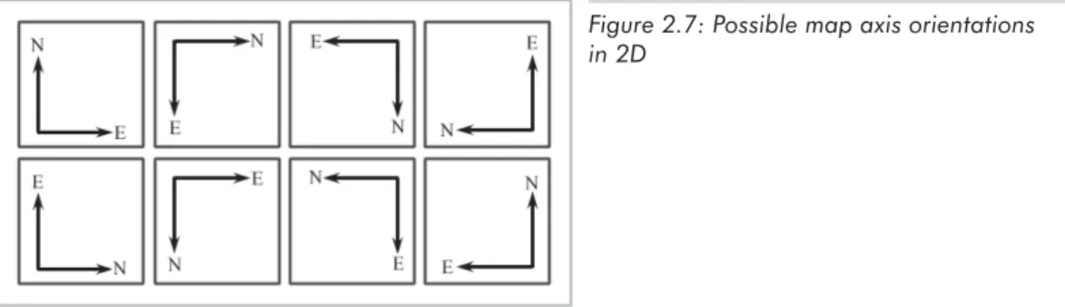
The committee quickly decided that there were only eight possible orientations that the mapmaker could deliver, shown in Figure 2.7. In the best of all possible worlds, he would deliver a map ori-ented as shown in the top-left rectangle, with north pointing to the top of the page and east to the right, which is what people usually expect. A subcommittee decided to name this the normal orientation.
After the meeting had lasted a few hours and tempers were beginning to fray, it was decided that the other three variants shown in the top row of Figure 2.7 were probably acceptable too, because they could be transformed to the normal orientation by placing a pin in the center of the page and rotating the map around the pin. (You can do this too by placing this book flat on a table
12
Chapter 2: The Cartesian Coordinate SystemFigure 2.6: Screen coordinate space
and turning it.) Many hours were wasted by tired functionaries putting pins into various places in the maps shown in the second row of Figure 2.7, but no matter how fast they twirled them, they couldn’t seem to transform them to the normal orientation. It wasn’t until everybody important had given up and gone home that a tired intern, assigned to clean up the used coffee cups, noticed that the maps in the second row could be transformed into the normal orientation by holding them up against a light and viewing them from the back. (You can do this too by holding Figure 2.7 up to the light and viewing it from the back. You’ll have to turn it too of course.) The writing was back-ward too, but it was decided that if Leonardo da Vinci (1452-1519) could handle backback-ward writing in the 15th century, then the citizens of Cartesia, though by no means his intellectual equivalent (probably due to daytime TV), could probably handle it in the 21st century also.
In summary, no matter what orientation we choose for thexandyaxes, we can always rotate the coordinate space around so that +xpoints to our right, and +ypoints up. For our example of screen-space coordinates, imagine turning upside down and looking at the screen from behind the monitor. In any case, these rotations do not distort the original shape of the coordinate system (even though we may be looking at it upside down or reversed). So in one particular sense, all 2D coordinate systems are “equal.” Later, we will discover the surprising fact that this is not the case in 3D.
2.2.3 Specifying Locations in 2D Using Cartesian
Coordinates
A coordinate space is a framework for specifying location precisely and mathematically. To define the location of a point in a Cartesian coordinate space, we use Cartesiancoordinates. In 2D, two numbers are used to specify a location. (The fact that we use two numbers to describe the location of a point is the reason it’s calledtwo-dimensional space. In 3D, we will use three numbers.) These two numbers are namedxandy. Analogous to the street names in Cartesia, each number specifies which side of the origin the point is on, and how far away the point is from the origin in a given direction. More precisely, each number is thesigned distance(that is, positive in one direction and negative in the other) to one of the axes, measured along a line parallel to the other axis. This may sound complicated, but it’s really very simple. Figure 2.8 shows how points are located in 2D Car-tesian space.
As shown in Figure 2.8, the xcoordinate designates the signed distance from the point to the y-axis, measured along a line parallel to the x-axis. Likewise, the y coordinate designates the signed distance from the point to the x-axis, measured along a line parallel to the y-axis. By “signed distance,” we mean that distance in one direction is considered positive, and distance in the opposite direction is considered negative.
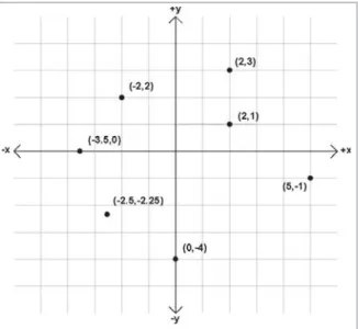
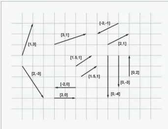
The standard notation that is used when writing a pair of coordinates is to surround the numbers in parentheses, with thexvalue listed first, like (x,y). Figure 2.9 shows several points and their Car-tesian coordinates. Notice that the points to the left of they-axis have negativexvalues, while those to the right of they-axis have positivexvalues. Likewise, points with positiveyare located above thex-axis, and points with negativeyare below thex-axis. Also notice thatanypoint can be specified, not just the points at grid line intersections. You should study this figure until you are sure that you understand the pattern.
2.3 From 2D to 3D
Now that we understand how Cartesian space works in 2D, let’s leave the flat 2D world and begin to think about 3D space. It might seem at first that 3D space is only 50 percent more complicated than 2D. After all, it’s justonemore dimension, and we already hadtwo. Unfortunately, this is not the case. For a variety of reasons, 3D space ismorethan incrementally more difficult for humans to visualize and describe than 2D space. (One possible reason for this difficulty could be that our physical world is 3D, while illustrations in books and on computer screens are 2D.) It is frequently the case that a problem that is “easy” to solve in 2D is much more difficult or even undefined in 3D. Still, many concepts in 2D do extend directly into 3D, and we will frequently use 2D to estab-lish an understanding of a problem and develop a solution, and then extend that solution into 3D.
14
Chapter 2: The Cartesian Coordinate System2.3.1 Extra Dimension, Extra Axis
In 3D, we require three axes to establish a coordinate system. The first two axes are called the x-axis andy-axis, just as in 2D. (However, it is not accurate to say that these are thesameas the 2D axes. We will discuss this more later.) We call the third axis (predictably) thez-axis. Usually, we set things up so that all axes are mutually perpendicular. That is, each one is perpendicular to the others. Figure 2.10 shows an example of a 3D coordinate space:
As discussed in Section 2.2.2, it is customary in 2D for +xto point to the right and +yto point up. (Sometimes +ymay point down, but in either case, thex-axis is horizontal and they-axis is verti-cal.) These are fairly standard conventions. However, in 3D, the conventions for arrangement of the axes in diagrams and the assignment of the axes onto physical dimensions (left, right, up, down, forward, back) are not very standardized. Different authors and fields of study have differ-ent convdiffer-entions. In Section 2.3.4 we will discuss the convdiffer-entions used in this book.
As mentioned earlier, it is not entirely appropriate to say that thex-axis andy-axis in 3D are the “same” as thex-axis andy-axis in 2D. In 3D, any pair of axes defines a plane that contains the two axes and is perpendicular to the third axis. (For example, the plane containing thex- and y-axes is thexyplane, which is perpendicular to thez-axis. Likewise, thexzplane is perpendicular to they-axis, and theyzplane is perpendicular to thex-axis.) We can consider any of these planes a 2D Cartesian coordinate space in its own right. For example, if we assign +x, +y, and +zto point right, up, and forward, respectively, then the 2D coordinate space of the “ground” is thexzplane.
2.3.2 Specifying Locations in 3D
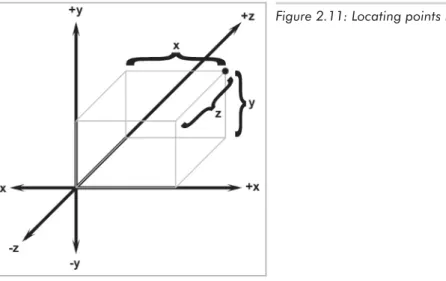
In 3D, points are specified using three numbers,x,y, andz, which give the signed distance to the yz,xz, andxyplanes, respectively. This distance is measured along a line parallel to the axis. For example, thex-value is the signed distance to theyzplane, measured along a line parallel to the
x-axis. Don’t let this precise definition of how points in 3D are located confuse you. It is a straight-forward extension of the process for 2D, as shown in Figure 2.11:
2.3.3 Left-handed vs. Right-handed Coordinate Spaces
As we discussed in Section 2.2.2, all 2D coordinate systems are “equal” in the sense that for any two 2D coordinate spaces A and B, we can rotate coordinate space A so that +xand +ypoint in the same direction as they do in coordinate space B. (We are assuming perpendicular axes.) Let’s examine this idea in more detail.
Figure 2.5 shows the “standard” 2D coordinate space. Notice that the difference between this coordinate space and “screen” coordinate space shown in Figure 2.6 is that they-axis points in opposite directions. However, imagine rotating Figure 2.6 clockwise 180°so that +ypoints up and +xpoints to the left. Now rotate it by “turning the page” and viewing the diagram from behind. Notice that now the axes are oriented in the “standard” directions like in Figure 2.5. No matter how many times we flip an axis, we can always find a way to rotate things back into the standard orientation.
Let’s see how this idea extends into 3D. Examine Figure 2.10 once more. Notice that +zpoints into the page. Does it have to be this way? What if we made +zpoint out of the page? This is cer-tainly allowed, so let’s flip thez-axis.
Now can we rotate the coordinate system around so that things line up with the original coor-dinate system? As it turns out, we cannot. We can rotate things to line uptwoaxes at a time, but the third axis always points in the wrong direction! (If you have trouble visualizing this, don’t worry. In a moment we will illustrate this principle in more concrete terms.)
All 3D coordinate spaces arenotequal; some pairs of coordinate systems cannot be rotated to line up with each other. There are exactly two distinct types of 3D coordinate spaces:left-handed coordinate spaces and right-handedcoordinate spaces. If two coordinate spaces have the same
16
Chapter 2: The Cartesian Coordinate Systemhandedness, then they can be rotated such that the axes are aligned. If they are of opposite handed-ness, then this is not possible.
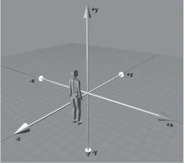
What exactly do “left-handed” and “right-handed” mean? First, let’s look at a simple and intu-itive way to identify the handedness of a particular coordinate system. The easiest and most illustrative way to identify the handedness of a particular coordinate system is to use, well, your hands! With your left hand, make an “L” with your thumb and index finger. (You may have to put the book down. . . .) Your thumb should be pointing to your right, and your index finger should be pointing up. Now extend your third finger so it points directly forward. (This may require some dexterity — don’t do this in public or you may offend someone!) You have just formed a left-handed coordinate system. Your thumb, index finger, and third finger point in the +x, +y, and +zdirections, respectively. This is shown in Figure 2.12.
Now perform the same experiment with your right hand. Notice that your index finger still points up, and your third finger points forward. However, with your right hand, your thumb will point to theleft. This is a right-handed coordinate system. Again, your thumb, index finger, and third fin-ger point in the +x, +y, and+zdirections, respectively. A right-handed coordinate system is shown in Figure 2.13.
Figure 2.12: Left-handed coordinate space
Try as you might, you cannot rotate your hands into a position so that all three fingers simulta-neously point the same direction on both hands. (Bending your fingers is not allowed. . . .)
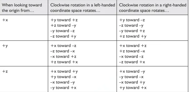
When looking toward the origin from…
Clockwise rotation in a left-handed coordinate space rotates…
Clockwise rotation in a right-handed coordinate space rotates…
+x +y toward +z
+z toward –y –y toward –z –z toward +y
+y toward –z –z toward –y –y toward +z +z toward +y
+y +x toward –z
–z toward –x –x toward +z +z toward +x
+x toward +z +z toward –x –x toward –z –z toward +x
+z +x toward +y
+y toward –x –x toward –y –y toward +x
+x toward –y –y toward –x –x toward +y +y toward +x
Now that we have discussed the intuitive definition of left- and right-handed coordinate systems, let’s discuss a more technical one based on clockwise rotation. Study the table shown in Figure 2.14. To understand how to read this table, examine the first row. Imagine that you are looking at the origin from the positive end of thex-axis. (You are facing the –xdirection.) Now imagine rotat-ing they-andz-axes clockwise about thex-axis. In a left-handed coordinate system, the positive end of they-axis rotates toward the positive end of thez-axis and the positive end of thez-axis rotates toward the negative end of they-axis, etc. This situation is illustrated in Figure 2.15.
18
Chapter 2: The Cartesian Coordinate SystemFigure 2.14: Comparison of left- and right-handed coordinate systems
Figure 2.15: Viewing a left-handed coordinate space from the positive end of the x-axis
TE
AM
FL
Y
In a right-handed coordinate system, the opposite occurs: the positive end of they-axis rotates toward the negative end of thez-axis, etc. The difference lies in which directions are considered “positive.” We are performing the same rotation in both cases.
Any left-handed coordinate system can be transformed into a right-handed coordinate system, or vice versa. The easiest way to do this is by swapping the positive and negative ends of one axis. Notice that if we fliptwoaxes, it is the same as rotating the coordinate space 180°about the third axis, which does not change the handedness of the coordinate space.
Both left-handed and right-handed coordinate systems are perfectly valid, and despite what you might read in other books, neither is “better” than the other. People in various fields of study certainly have preferences for one or the other depending on their backgrounds. For example, tra-ditional computer graphics literature typically uses left-handed coordinate systems, whereas the more math-oriented linear algebra people tend to prefer right-handed coordinate systems. Of course, these are gross generalizations, so always check to see what coordinate system is being used. The bottom line, however, is that it’s just a matter of a negative sign in thezcoordinate. So, appealing to the First Law of Computer Graphics in Section 2.1, if you apply a tool, technique, or resource from another book, web page, or article and it doesn’t look right, try flipping the sign on thezaxis.
2.3.4 Some Important Conventions Used in This Book
When designing a 3D virtual world, there are several design decisions that we have to make beforehand, such as left-handed or right-handed coordinate system, which direction is +y, etc. The mapmakers from Dyslexia had to choose from among eight different ways to assign the axes in 2D (see Figure 2.7). In 3D, we have a total of 48 different combinations to choose from. Twenty-four of these combinations are left-handed, and 24 are right-handed.
Different situations can call for different conventions in the sense that certain things can be easier if you adopt the right ones. Usually, however, it is not a major deal as long as you establish the conventions early in your design process and stick to them. All of the basic principles dis-cussed in this book are applicable, regardless of the conventions used. For the most part, all of the equations and techniques given are applicable regardless of convention as well. However, in some cases there are some slight, but critical, differences in application dealing with left-handed versus right-handed coordinate spaces. When those differences arise, they will be pointed out.
In situations where “right” and “forward” are not appropriate terms (for example, when we dis-cuss the world coordinate space), we will assign +xto “east” and +zto “north.”
2.4 Exercises
1. Give the coordinates of the following points:
20
Chapter 2: The Cartesian Coordinate SystemFigure 2.16: The left-handed coordinate system conventions used in this book
2. List the 48 different possible ways that the 3D axes may be assigned to the directions “north,” “east,” and “up.” Identify which of these combinations are left-handed and which are right-handed.
Multiple Coordinate
Multiple Coordinate
Spaces
In Chapter 2, we discussed how we can establish a coordinate space anywhere we want simply by picking a point to be the origin and deciding on the directions we want the axes to be oriented. We usually don’t make these decisions arbitrarily; we form coordinate spaces for specific reasons (one might say “different spaces for different cases”). This chapter gives some examples of com-mon coordinate spaces that are used for graphics and games. We will then discuss how coordinate spaces are nested within other coordinate spaces.
23
This chapter introduces the idea of multiple coordinate systems. It is divided into five main sections.
n Section 3.1 justifies the need for multiple coordinate systems.
n Section 3.2 introduces some common coordinate systems. The main concepts intro-duced are:
u World space
u Object space
u Camera space
u Inertial space
n Section 3.3 discusses nested coordinate spaces, commonly used for animating hier-archically segmented objects in 3D space.
n Section 3.4 describes how to specify one coordinate system in terms of another.
n Section 3.5 describes coordinate space transformations. The main concepts are:
u Transforming between object space and inertial space
3.1 Why Multiple Coordinate Spaces?
Why do we need more than one coordinate space? After all, anyone3D coordinate system extends infinitely and thus contains all points in space. So we could just pick a coordinate space, declare it to be the “world” coordinate space, and all points could be located using this coordinate space. Wouldn’t that be easier? In practice, the answer to this is “no.” Most people find it more conve-nient to use different coordinate spaces in different situations.
The reason multiple coordinate spaces are used is that certain pieces of information are only known in the context of a particular reference frame. It is true that, theoretically, all points could be expressed using a single “world” coordinate system. However, for a certain pointa, we may not know the coordinates ofain the “world” coordinate system. However, we may be able to express ausing someothercoordinate system. For example, the residents of Cartesia (see Section 2.2.1) use a map of their city with the origin centered, quite sensibly, at the center of town and the axes directed along the cardinal points of the compass. The residents of Dyslexia use a map of their city with the coordinates centered at an arbitrary point and the axes running in some arbitrary direction that probably seemed like a good idea at the time. The citizens of both cities are quite happy with their respective maps, but the State Transportation Engineer assigned the task of running up a bud-get for the first highway between Cartesia and Dyslexia needs a map showing the details of both cities, which introduces a third coordinate system that is superior tohim, though not necessarily to anybody else. The major points on both maps need to be translated from the local coordinates of the respective city to the new coordinate system to make the new map.
The concept of multiple coordinate systems has historical precedent. While Aristotle (384-322 BCE), in his booksOn the HeavensandPhysics, proposed ageocentricuniverse with the Earth at the origin, Aristarchus (ca. 310-230 BCE) proposed aheliocentricuniverse with the Sun at the origin. So we can see that more than two millennia ago the choice of coordinate system was already a hot topic for discussion. The issue wasn’t settled for another couple of millennia until Nicholas Copernicus (1473-1543) observed in his book De Revolutionibus Orbium Coelestium (“On the Revolutions of the Celestial Orbs”) that the orbits of the planets can be explained more simply in a heliocentric universe without all the mucking about with wheels within wheels in a geocentric universe. Of course, not everybody could appreciate the math, which is what got Galileo Galilei (1520-1591) in so much trouble during the Inquisition, since the church had reasons of its own (having little if anything to do with math) for believing in a geocen-tric universe.
In Sand-Reckoner,Archimedes (d. 212 BCE), perhaps motivated by some of the concepts
introduced in Section 2.1, developed a notation for writing down very large numbers, numbers much larger than anybody had ever counted to at that time. Instead of choosing to count dead sheep as in Section 2.1, he chose to count the number of grains of sand that it would take to fill the universe. (He estimated that it would take 8x1063grains of sand, but he did not, however, address the question of where we would get the sand from.) In order to make the numbers larger, he chose Aristarchus’ revolutionary new heliocentric universe rather than the geocentric universe generally accepted at the time. In a heliocentric universe, the Earth orbits the Sun, in which case the fact that the stars show no parallax means that they must be much farther away than Aristotle could ever
have imagined. To make his life more difficult, Archimedes deliberately chose the coordinate sys-tem that would produce larger numbers. We will use the direct opposite of his approach. In creating our virtual universe inside the computer, we will choose coordinate systems that make our liveseasier, notharder.
In today’s enlightened times, we are accustomed to hearing in the media aboutcultural rela-tivism, which promotes the idea that it is incorrect to consider one culture or belief system or national agenda to be superior to another. It’s not too great a leap of the imagination to extend this to what we might call “transformational relativism,” that no place, orientation, or coordinate sys-tem can be considered superior to others. In a certain sense, that’s true, but to paraphrase George Orwell inAnimal Farm, “All coordinate systems are considered equal, but some are more equal than others.” Let’s look at some examples of common coordinate systems that you will meet in 3D graphics.
3.2 Some Useful Coordinate Spaces
Different coordinate spaces are needed because some information is only meaningful in a particu-lar context.
3.2.1 World Space
One of the authors of this book wrote in Lewisville, Texas (near Dallas and Fort Worth). More pre-cisely, his location is:
n Latitude: 33° 01’ North
n Longitude: 96° 59’ West
The other author wrote in Denton, Texas, at:
n Latitude: 33° 11’ North
n Longitude: 97° 07’ West
These values express our “absolute” position in the world. You don’t need to know where Denton, Lewisville, Texas, or even the United States is to use this information because the position is abso-lute. (The astute reader will note that these coordinates are not Cartesian coordinates, but rather, they arepolarcoordinates. That is not significant for this discussion — we live in a flat 2D world wrapped around a sphere, a concept that supposedly eluded most people until Christopher Colum-bus verified it experimentally.) The origin, or (0,0) point in the world, was decided for historical reasons to be located on the equator at the same longitude as the Royal Observatory in the town of Greenwich, England.
Theworld coordinate systemis a special coordinate system that establishes the “global” refer-ence frame for all other coordinate systems to be specified. In other words, we can express the position of other coordinate spaces in terms of the world coordinate space, but we cannot express the world coordinate space in terms of any larger, outer coordinate space.
example, if we wanted to render a view of Cartesia, for all practical purposes Cartesia would be “the world,” since we wouldn’t care where Cartesia is located (or even if it exists at all). In differ-ent situations, your world coordinate space will define a differdiffer-ent “world.” In Section 4.3.1 we will discuss how “absolute position” is technically undefined. In this book, we will use the term “absolute” to mean “absolute with respect to the largest coordinate space we care about.” In other words, “absolute” to us will mean “expressed in the world coordinate space.”
The world coordinate space is also known for obvious reasons as theglobaloruniversal coor-dinate space.
Some examples of questions that are typically asked in world space include questions about initial conditions and the environment, such as:
n What is the position and orientation of each object?
n What is the position and orientation of the camera?
n What is the terrain like in each position in the world? (For example, hills, mountains, build-ings, lakes.)
n How does each object get from where it is to where it wants to be? (Motion planning for nonplayer characters.)
3.2.2 Object Space
Object space is the coordinate space associated with a particular object. Every object has its own independent object space. When an object moves or changes orientation, the object coordinate space associated with that object is carried along with it, so it moves or changes orientation too. For example, we all carry our own personal coordinate system around with us. If we were to ask you to “take one step forward,” we are giving you an instruction in your object space. (Please for-give us for referring to you as an object.) We have no idea which way you will move in absolute terms. Some of you will move north, some south, and others in different directions. Concepts such as “forward,” “back,” “left,” and “right” are meaningful in object coordinate space. When some-one gives you driving directions, sometimes you are told to “turn left” and other times you are told to “go east.” “Turn left” is a concept that is expressed in object space, and “east” is expressed in world space.
Locations can be specified in object space as well as directions. For example, if I asked you where the muffler on your car was located, you wouldn’t tell me “in Chicago,” even if you lived in Chicago. I’m asking where it iswithin your car. In other words, I want you to express the location of your muffler in the object space of your car.
In certain contexts, object space is also known asmodeling space, since the coordinates for the vertices of a model are expressed in modeling space. It is also known asbody space.
Some examples of questions that can be asked in object space are:
n Is there another object near me that I need to interact with? (Do I need to kill it?)
n In what direction is it? Is it in front of me? Slightly to my left? To my right? (So I can shoot at it or run in the opposite direction.)
3.2.3 Camera Space
Camera space is the coordinate space associated with an observer. Camera space is similar to screen space except that camera space is a 3D space, whereas screen space is a 2D space. Camera space can be considered a special object space, where the “object” that defines the coordinate space is the camera defining the viewpoint for the scene. In camera space, the camera is at the ori-gin with +xpointing to the right, +zpointing forward (into the screen, or the direction the camera is facing), and +ypointing “up” (not “up” with respect to the world, but “up” with respect to the top of the camera). Figure 3.1 shows a diagram of camera space.
Note that other books may use different conventions for the orientation of the axes in camera space. In particular, many graphics books that use a right-handed coordinate system point –zinto the screen, with +zcoming out of the screen toward the viewer.
Typical questions asked in camera space include queries about what is to be drawn on the screen (graphics questions), such as:
n Is a given point in 3D space in front of the camera?
n Is a given point in 3D space on screen, or is it off to the left, right, top, or bottom edges of the camera frustum? (Thefrustumis the pyramid of space that can be seen by the camera.)
n Is an object completely on screen, partially on screen, or completely off screen?
n Which of the two objects is in front of the other? (This is calledocclusioninformation.) Notice that the answers to these questions are critical if we wish to render anything. In Section 15.3 we will learn how 3D camera space is related to 2D screen space through a process known as projection.

![Figure 4.7 illustrates how the point (x, y) is related to the vector [x, y], given arbitrary values for x and y.](https://thumb-us.123doks.com/thumbv2/123dok_us/8182744.2169214/54.810.166.446.629.876/figure-illustrates-point-related-vector-given-arbitrary-values.webp)
