IN THE PURSUIT OF SONS:
SEX-SELECTIVE ABORTION AND DIFFERENTIAL STOPPING IN PAKISTAN
Batool Zaidi
A thesis submitted to the faculty at the University of North Carolina at Chapel Hill in partial fulfillment of the requirements for the degree of Master of Arts in the Department of Sociology
in the College of Arts and Sciences.
Chapel Hill 2013
iii ABSTRACT
Batool Zaidi: In the Pursuit of Sons: Sex-Selective Abortion and Differential Stopping in Pakistan (Under the direction of S. Philip Morgan)
iv
ACKNOWLEDGEMENTS
v
TABLE OF CONTENTS
LIST OF TABLES ... vii
LIST OF FIGURES ... viii
LIST OF ABBREVIATIONS ... ix
CHAPTER 1: INTRODUCTION ... 1
CHAPTER 2: THE FERTILITY TRANSITION AND SEX PREFERENCE ... 3
CHAPTER 3: THE PAKISTANI EXPERIENCE ... 6
3.1 Fertility Squeeze ... 6
3.2 Son Preference ... 6
3.3 Availability of Technology ... 7
CHAPTER 4: DATA ... 10
CHAPTER 5: METHODS AND MEASURES ... 11
CHAPTER 6: RESULTS ... 13
6.1 Expected Probabilities ... 13
6.2 Evidence of Sex Selection ... 15
vi
CHAPTER 7: DISCUSSION ... 30
vii
LIST OF TABLES
Table 1: Probability of achieving compositional fertility goals
and the actual proportions of various compositions at each parity over time ... 14
Table 2: Sex ratios at births for women in the five years prior
to the survey, by background characteristics ... 16
Table 3: Sex ratios at births in the five years prior to the survey,
by number of previous siblings that are boys (2007) ... 18
Table 4: Calculation for number of sex-selective abortions for
different levels of sex ratios at birth ... 19
Table 5: Parity progression ratios for currently married women
with no birth in the last five years, by parity and gender composition of previous children ... 20
Table 6: Odds ratios for progressing to next birth ... 22
Table 7: Current Use of contraception, by gender composition
of children ... 24
Table 8: Logistic regression coefficients for current use of
contraception ... 25
Table 9: Intention to have no more children, by gender
composition of previous children ... 27
Table 10: Logistic regression coefficients for intention to stop
viii
LIST OF FIGURES
Figure 1: Expected patterns of sex ratios over the course
of the transition in son preference ... 3
Figure 2: Possible responses to conflicting pressures of
smaller family size and bearing a male offspring ... 8
Figure 3: Difference between expected and observed
ix
LIST OF ABBREVIATIONS
CI confidence interval
CPR contraceptive prevalence rate
DHS Demographic Health Survey
DSRB desired sex ratio at birth
EFB expected female births
FB female births
LB live births
MB male births
NIPS National Institute of Population Studies
PDHS Pakistan Demographic Health Survey
SRB sex ratio at birth
SRLB sex ratio at last birth
SSA sex-selective abortion
TFR total fertility rate
1
CHAPTER 1: INTRODUCTION
Given Pakistan’s geo-political importance, the future of its population is of great interest to academics as well as policymakers. Even if Pakistan’s fertility continues to decline and
reaches replacement level in the next 30 years, its population will have increased by a 100 million to around 275 million. This growth will make it the fifth most populous nation in the world (United Nations [UN], Department of Economic and Social Affairs, Population Division 2011). If son preference continues to be a strong determinant of fertility behavior, fertility levels will be increased by the pursuit of a male birth, making it harder for Pakistan to reach replacement fertility. Alternatively, if couples respond by using sex-selective abortion, Pakistan will experience skewed sex ratios possibly leading to additional social problems. A continuingly low contraceptive prevalence rate (CPR) of 35 percent (National Institute of Population Studies [NIPS] and Macro International 2013) and an elevated sex ratio at birth (SRB) (Guilmoto 2009) suggest both scenarios are unfolding.
2
3
CHAPTER 2: THE FERTILITY TRANSITION AND SEX PREFERENCE
The link between fertility and son preference changes over the course of the
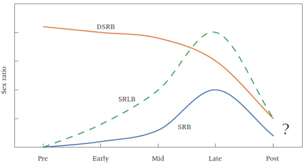
demographic transition. At the beginning of the transition when fertility control is low and women are having a large number of children, son preference is not a strong determinant of fertility behavior, even in patriarchal societies. As contraceptive technology becomes widely available and fertility starts declining, the preference for sons becomes an increasingly central factor in couples’ fertility decisions in such societies. This has been referred to by some as the “intensification effect” of fertility decline on gender bias – when the fertility starts to decline “the total number of children couples desire falls more rapidly than the total number of desired sons” (Das Gupta and Bhat 1997). Bongaarts’ (2013) paper shows the changing relationship between the fertility transition and the desire and observed preference for sons (see Figure 1).
Figure 1: Expected patterns of sex ratios over the course of the transition in son preference
4
At higher parities, the probability of having at least one son is very high (Dyson 2012). However, as family size gets smaller, the probability of having a son gets smaller. When the average family size is six children, the probability of being sonless is one percent. However, when the average family size falls to three children, the probability of being sonless increases to 12 percent (Bongaarts and Potter 1983). The probability of being sonless doubles with every one child reduction in the average family size (Guilmoto 2009). In other words, in order to ensure at least one son, women would need to have 1.94 births on average, and in order to have at least two sons, they would need to have 4.38 births on average (Bongaarts and Potter 1983). Guilmoto (2009) argues that as low fertility norms set deeper into society the marginal costs of additional children become increasingly untenable. In order to ensure both size and
compositional goals couples resort to sex-selective abortion.
Higher than normal sex ratios at birth are “unambiguous evidence” that couples are practicing sex-selective abortions (Bongaarts 2013). Note that differential stopping behavior – when women stop childbearing through contraceptive use if they have achieved the desired number of sons or continue childbearing till they have the desired number of sons– does not translate to skewed sex ratios at birth. This is because the probability of having a son or daughter remains largely fixed, regardless of parity.1In contrast, sex-selective abortion alters the number of boys being born, thus producing skewed sex ratios at birth.
Over the last decade and half skewed sex ratios at birth have been reported in several Asian countries. Much of the research on sex ratio imbalances focused on South Korea, India and China where national sex ratios at birth deviated from normal levels of 106 to as high as 115, 119, and 110, respectively, (Hesketh and Xing 2006). Since then, elevated sex ratios have been reported in other Asian countries including Vietnam (Guilmoto 2012), Azerbaijan,
Armenia, Georgia, and Albania (Duthé et al. 2012). All countries experiencing elevated sex ratios at birth have low fertility and abortion technology widely available.
1There is evidence of a slight dependence of sex of birth to sex composition of previous births – this is
5
Even though Pakistan continues to be a highly patriarchal society, it has not featured prominently in studies focusing on son preference and sex ratios at birth because, until
6
CHAPTER 3: THE PAKISTANI EXPERIENCE 3.1 Fertility Squeeze
While most of its neighboring countries began experiencing fertility decline before the 1980s, fertility rates in Pakistan remained above six births per woman until the late 1980s/early 1990s. It is widely accepted that the fertility transition in Pakistan began at this point (Sathar and Casterline 1998). Despite a significant drop after the onset, overall fertility in Pakistan declined slowly throughout the 1990s, and reached 4.8 births per woman by 2000–01.
Given the high number of children women were having, it is not surprising that son-preference did not translate into high sex ratios at birth (Hesketh and Xing 2006) during this time period. In the last decade however, Pakistan’s total fertility rate (TFR) has declined further and is estimated to be around 3.8 births per woman, and is as low as 3.2 in urban areas (NIPS and Macro International 2013). Women in Pakistan are now facing the fertility squeeze that makes achieving sex preferences difficult without preferential behavior.
3.2 Son Preference
7
Using data from the Pakistan Demographic Health Survey (PDHS), Bharadwaj and Lakdawala (2013) find that women are more likely to get prenatal checkups and take iron pills when pregnant with a boy. The magnitude of discrimination is larger in areas with more son preference.
It is not surprising then, that of 61 countries, Pakistan has the second highest desired sex ratio at birth (DSRB), a measure of the preference for sons calculated using reported ideal number of male and female offspring by couples in Demographic and Health Surveys
(Bongaarts 2013).
3.3 Availability of Technology
For the high DSRB to translate into high SRB, couples need to have the means to identify the sex of a fetus and have access to abortion services (Bongaarts 2013). Contrary to
expectations, abortion rates in Pakistan are unexpectedly high for an Islamic country that forbids abortion under all, but extreme circumstances. A national study found abortion rates in Pakistan to be much higher than expected; an estimated 890,000 abortions took place in 2002 – amounting to 29 abortions per 1,000 women of reproductive age (Sathar, Singh, and Fikree 2007). According to a study of women hospitalized for post-abortion complications, 20 percent of women who had an abortion had 0–2 children, and another 30 percent had 3–4 children (Vlassoff, Singh, and Suarez 2009). Given that the ideal family size was close to four children, it is likely that not all of these abortions were for limiting family size.
The 2007 PDHS shows that ultrasound technology is widely available in urban and rural areas – 66 percent of women had an ultrasound check during antenatal checkup for their last pregnancy (NIPS and Macro International 2008). These findings indicate both the availability of services and women’s willingness to seek abortions despite cultural taboos – a trend that is likely to have increased over the last decade.
8
prerequisites do not guarantee sex-selective abortions; it is possible that Pakistani women may be differentially choosing to continue childbearing in order to achieve compositional goals.
According to Bongaarts’ study (2013), Pakistan also had the fifth highest sex ratio at last birth (SRLB). A high SRLB is a very sensitive indicator of differential stopping behavior, and can be explained entirely by differential contraceptive use. The CPR increased rapidly from around 11 percent in 1991 to 33 percent by 2003. But by 2007, it had not increased further and had in fact declined slightly to 29 percent. The latest round of the DHS (2012–13) reports a CPR of 35 percent. Stalling CPRs and the consequent slowdown of fertility decline indicate that women may be continuing childbearing in the pursuit of sons.
As fertility continues to fall and women get closer to achieving their desired family size but son preference remains pervasive, the role of compositional goals in fertility decisions is expected to continue to increase. So in the face of persistent son preference, but changing family size norms, are Pakistani women ignoring cultural pressures and compositional goals, having more children, or getting an abortion to meet both size and compositional fertility goals (Figure 2)?
Figure 2: Possible responses to conflicting pressures of smaller family size and bearing a male offspring
Son Preference Smaller Family Size
Additional births till son Sex selective abortion Change sex preference
Skewed sex-ratios at birth
9
10 CHAPTER 4: DATA
In the absence of recent census data, I study these questions by using data from two rounds (1990–91 and 2006–07) of the PDHS. Data from demographic and health surveys has been used in several international research studies on son preference and prenatal sex selection (Arnold, Kishor, and Roy 2002; Ebenstein 2007; Garenne 2008; Bongaarts 2013).
The demographic and health surveys collect data on the reproductive history, behavior, and intentions for women of reproductive age (15–49). The PDHS sample for 1990–91
comprised of 6,611 ever-married women (15–49) and their birth history data for 27,369 births2. The 2006–07 sample was larger, containing information on 10,032 ever-married women (15–49) and all their births (39,049).
The birth history data provide the gender and birth order of each birth allowing for the estimation of parity progression ratios by gender composition of previous births. The data on intentions allow for a more prospective analysis of the relationship between son-preference and fertility. The detailed background indicators collected in the PDHS provide an opportunity to study these patterns across various population subgroups. And importantly, the two rounds of the survey allow for a comparison of these measures over the time Pakistan has experienced the fertility transition.3
2The 1990–91 DHS data was argued to have severely underestimated fertility rates (Juarez and Sathar
2001). The re-interview survey conducted to check data reliability did find evidence of underreporting of births, but none for sex differentials in consistency of reporting (Curtis and Arnold 1994). These problems suggest caution in interpreting the 1990–91 results but do not suggest a particular bias in key results presented here.
3Fieldwork for another round of the PDHS has reached completion and findings/data will be made
11 CHAPTER 5: METHODS AND MEASURES
The bulk of the analysis in the paper is based on the sex of a child being a random event with relatively fixed probabilities of being a boy (0.512) or a girl (0.488)4. I use Bongaarts and Potter’s (1983) work on expected probabilities of achieving particular compositional fertility goals in the absence of pre-selection to test whether the observed compositional (based on gender) distribution at each parity is different from the expected distribution, and whether these differences have changed over time. I use the binomial test to check for statistical
significance of the differences between observed and expected. The binomial test is appropriate with small samples where approximations of continuous distribution breakdown. Differences in the expected and observed proportions could be a result of either sex-selective stopping
behavior or sex-selective abortions, or both; I measure these responses next.
I calculate sex ratios at birth by education, rural-urban residence, household wealth status, and birth parity for all births in the five years previous to the survey for both time periods.5 These differentials help highlight the prevalence of sex ratio imbalances in groups most at risk of practicing prenatal sex-selection, as shown in previous studies on countries with high sex ratios (Guilmoto 2007; Filmer, Friedman, and Schady 2009). Comparing the sex ratios across the two survey rounds helps determine whether sex ratios are increasing or not, thereby offering evidence for, or against the use of sex-selective abortion.
4In the initial analyses, I made use of the slight dependency for the sex of the next birth to be like that of
prior births (i.e., Ps= 51.45+ 0.3Ns - 0.5Nd, where Ps = percent sons; Ns = number of prior sons; Nd=number of prior daughters, see Bongaarts and Potter 1983: 204). However, because the probabilities under the assumption of independence lead to more conservative estimate of preferential treatment than those under the assumption of slight dependency, we only present the results for the former.
5Similar to other studies (Guilmoto 2007; 2009), I limit the calculation to births five years before the
12
Estimating the SRB can be difficult due to this statistical indicator’s sensitivity to sample size (Guilmoto 2009). The SRB needs to be calculated using a large number of births to avoid fluctuations within large confidence intervals. A sex ratio of 106 calculated using survey data with a sample of 10,000 has a 95 percent confidence interval of 102–110 (Arnold, Kishor, and Roy 2002). The confidence intervals for a normal sex ratio of 106, given the sample size, are calculated for each subsample to check whether the estimated SRB is outside this range. I also used the alternative approach – the one-tailed binomial test – for testing whether the calculated sex ratios at births are significantly different from 106. Even though my hypotheses are
directional in nature (more boys than girls, i.e. higher than normal SRBs) and thus subject to one-tailed tests, only confidence intervals are presented in this paper because they offer a more conservative estimate of significance. Additionally, chi-square tests are applied to test whether the elevated SRBs were statistically different from other SRBs across different parities.
The second part of the analysis focuses on measuring differential stopping. I look at how the gender composition of previous children influences the probability of continuing childbearing (parity progression ratios) as well as the probability of using contraception. Alongside this, I include a more prospective approach similar to that of Pollard and Morgan (2002) for analyzing the link between son-preference and fertility outcomes by studying fertility intentions.
Logistic regression models are used to statistically test the effect of sex composition of previous siblings/children on fertility behavior (progression and contraceptive use) and
13 CHAPTER 6: RESULTS
6.1 Expected Probabilities
14
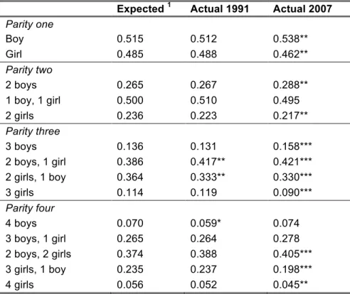
Table 1: Probability of achieving compositional fertility goals and the actual proportions of various compositions at each parity over
time
Expected 1 Actual 1991 Actual 2007
Parity one
Boy 0.515 0.512 0.538**
Girl 0.485 0.488 0.462**
Parity two
2 boys 0.265 0.267 0.288**
1 boy, 1 girl 0.500 0.510 0.495 2 girls 0.236 0.223 0.217**
Parity three
3 boys 0.136 0.131 0.158***
2 boys, 1 girl 0.386 0.417** 0.421*** 2 girls, 1 boy 0.364 0.333** 0.330*** 3 girls 0.114 0.119 0.090***
Parity four
4 boys 0.070 0.059* 0.074
3 boys, 1 girl 0.265 0.264 0.278 2 boys, 2 girls 0.374 0.388 0.405*** 3 girls, 1 boy 0.235 0.237 0.198*** 4 girls 0.056 0.052 0.045**
1 Assuming the probability of a boy is 0.5145 and independent of gender
composition of previous births.
Table 1 shows the proportions of women with specific gender compositions across parities one to four over time. We find that while most of the observed proportions were not statistically different from the expected probabilities in 1991, the situation changes
dramatically in 2007. In the later time period, the proportion of women having all, or a majority of daughters within each family size is significantly lower than would be expected, given the fixed probabilities of having a girl or a boy6. The differences between expected and observed proportions is highest at parity three and parity 4 four. The proportion of women with three children who have only daughters is expected to be 0.114; in 1991, the observed proportion is 0.119, very close to the proportion (and not statistically different). However, by 2007, this proportion has decreased to 0.09. The difference is even more pronounced for women who
15
have two girls and one boy – 0.330 compared to the expected 0.366. For women with four children, once again, there are fewer women with a majority of girls (three or more) than expected in 2007. These differences can be seen more clearly in Figure 3.
Figure 3: Difference between expected and observed distribution gender composition by parity
* p < 0.1; ** p < 0.05 ; *** p < 0.01
While the disproportionate small proportion of families with no or one son point towards some sort of sex preferential behavior, it does not tell us whether this is a result of differential stopping behavior or sex selective abortion. For example, it may be that couples with no sons go on to the next parity while those two sons stop. This would lead a fewer two daughter families and more two son families among two children families. I present evidence on both responses in the following sections.
6.2 Evidence of Sex Selection
Table 2 shows that the SRB for the five years preceding the survey increased from 101 in 1991 to 110 in 2007. The shift from normal to elevated SRB corresponds to the timing of the decline in fertility rates – as noted in the introduction, fertility decline in Pakistan began in the early 1990s and had declined dramatically by 2007. It should be noted that I find no clear
* ** * ** *** *** *** *** ** ** *** ** -0.06 -0.05 -0.04 -0.03 -0.02 -0.01 0.00 0.01 0.02 0.03 0.04 0.05
3B 2B,1G 2G,1B 3G 4B 3B,1G 2B,2G 3G,1B 4G
1991 2007
16
evidence of elevated sex ratios for any sub-population (e.g., by region, parity, or education) in 1991. Even though most of the elevated SRBs in 2007 are not significant due to small Ns, the uniform increase is consistent with the emergence of sex-selective abortion.
Table 2: Sex ratios at births for women in the five years prior to the survey, by background characteristics
1991 2007
n SRB 95% CI for 106 n SRB 95% CI for 106
Overall 6,426 101 100.9 111.3 9,112 110 101.7 110.4
Region
Urban 3,373 100 99.1 113.4 3,116 115** 98.8 113.7
Rural 3,053 104 98.7 113.8 5,996 108 100.7 111.5
Mother’s education
None 4,878 102 100.2 112.1 6,178 112** 100.8 111.4
Primary 1–5
634 95 90.7 123.9 1,224 102 94.7 118.6
Secondary 6–10
828 104 92.5 121.5 1,163 104 94.5 118.9
Higher 10+
86 (-) 69.2 163.2 547 118 89.6 125.4
Birth order
1 1,126 115 94.3 119.2 1,880 108 96.8 116.0 2 1,021 106 93.7 119.9 1,673 110 96.3 116.7 3 944 99 93.3 120.5 1,397 125** 95.4 117.7 4 817 94 92.4 121.6 1,165 113 94.5 118.9 5+ 2,518 97 98.0 114.6 2,997 105 98.7 113.9
CI = confidence interval
Assuming independence p (boy) = 0.5145
*p<0.1; **p<0.05 à 106 significantly different from SRB
17
106, the SRB of 118 for women with higher education is not. This is due to the smaller sample size of the higher education group.
Looking at sex ratio by birth-order provides stronger evidence of sex-selection in Pakistan. While sex ratios have remained largely unchanged for lower parities (one or two) and high parities (five or more), sex ratios have increased substantially at third and fourth births, coinciding with the reported ideal number of children. Even with a sample size of less than 1,400 births, a SRB of 125 at third births is significantly higher than normal levels. And although the SRB of 113 at parity four in 2007 is not statistically different from 106, it is substantially larger than the SRB of 94 in 1991.
In Table 3, I calculate SRB by birth-order and the number of previous sons. These calculations allow us to look for evidence of elevated sex ratios where one would most expect to find them – among those with several children but no sons. The estimates in Table 3 confirm our suspicion in the 2006–07 data. The sex ratio is significantly different from 106 and highest (134) for those with three children but no previous sons. Depending on how significance is calculated, SRBs are significantly elevated at parity two and three births with one previous son7. This again hints at a preference for two boys among Pakistani couples. A chi-square statistic of 12.4 indicates that the SRB of 134 is also significantly different from the sex ratio for all other parities combined.
7Had I assumed that the probability of a male birth was dependent on sex of previous births, the elevated
18
Table 3: Sex ratios at births in the five years prior to the survey, by number of previous siblings that are boys (2007)
Birth order n SRB 95% CI for 106
No previous sons
1 1,880 108 96.8 116.0 2 810 100 92.3 121.7 3 346 134** 85.8 131.0 4+ 230 98 81.8 137.6
1 previous son
2 863 119 92.7 121.2 3 662 121 91.0 123.5 4+ 878 117 92.8 121.0
2 or more previous sons 3 389 125 86.9 129.4 4+ 3,054 105 92.7 121.2
Assuming independence p (boy)=0.5145
*p<0.1; **p<0.05à 106 significantly different from SRB
19
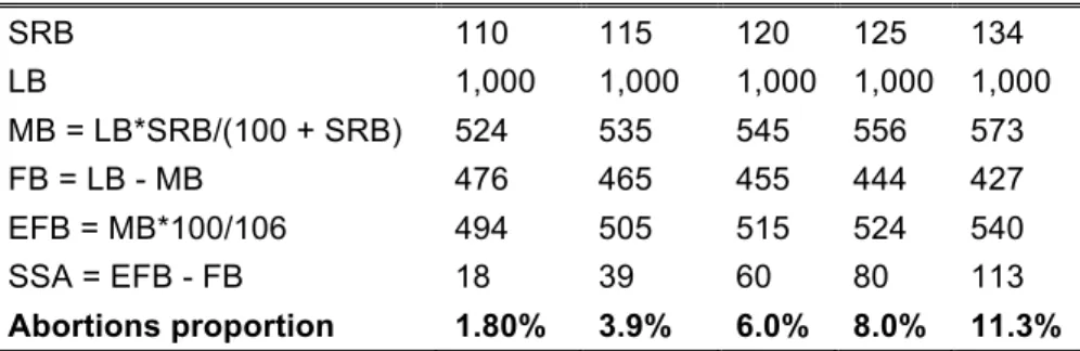
Table 4: Calculation for number of sex-selective abortions for different levels of sex ratios at birth
SRB 110 115 120 125 134
LB 1,000 1,000 1,000 1,000 1,000 MB = LB*SRB/(100 + SRB) 524 535 545 556 573 FB = LB - MB 476 465 455 444 427 EFB = MB*100/106 494 505 515 524 540 SSA = EFB - FB 18 39 60 80 113
Abortions proportion 1.80% 3.9% 6.0% 8.0% 11.3%
SRB = Sex ratio at birth; LB = live births; MB = male births; FB = female births; EFB = Expected female births; SSA = sex-selective abortions
6.3 Evidence of Stopping Behavior
6.3.1 Parity progression
In order to assess the level of stopping behavior I turn to an analysis of parity
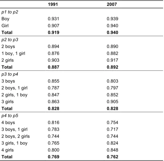
progression ratios. I limit my sample to women who have had no birth in the last five years so that the progression ratios reflect fertility behavior of women who have likely completed their desired family8.
The differences in parity progression ratios by sex composition of previous births for the two time periods are presented in Table 5. Three interesting patterns emerge from this table. First, progression ratios among women with all or majority daughters are higher than for those with all or majority sons. In 1991, the ratio of moving from parity two to parity three was .894 for women with only boys and .903 for those with only girls (a ratio of 1.01), these ratios changed to .890 and .917 in 2007 (1.03 ratio).
8Analysis is limited to women with no births in the last five years in order to capture women who have
20
Table 5: Parity progression ratios for currently married women with no birth in the last five years, by parity and gender composition of
previous children
1991 2007
p1 to p2
Boy 0.931 0.939
Girl 0.907 0.940
Total 0.919 0.940
p2 to p3
2 boys 0.894 0.890
1 boy, 1 girl 0.876 0.882
2 girls 0.903 0.917
Total 0.887 0.892
p3 to p4
3 boys 0.855 0.803
2 boys, 1 girl 0.787 0.797 2 girls, 1 boy 0.847 0.852
3 girls 0.863 0.905
Total 0.828 0.828
p4 to p5
4 boys 0.816 0.754
3 boys, 1 girl 0.783 0.717 2 boys, 2 girls 0.744 0.744 3 girls, 1 boy 0.765 0.824
4 girls 0.800 0.848
Total 0.769 0.762
This brings us to the second interesting pattern; differences in parity progression by gender composition have become more acute over the two time periods. While the difference was less than 0.009 in 1991, it increased to 0.023 in 2007. The increase in son preference over time is seen in progression from three to four children even more starkly; in 1991, the
21
22
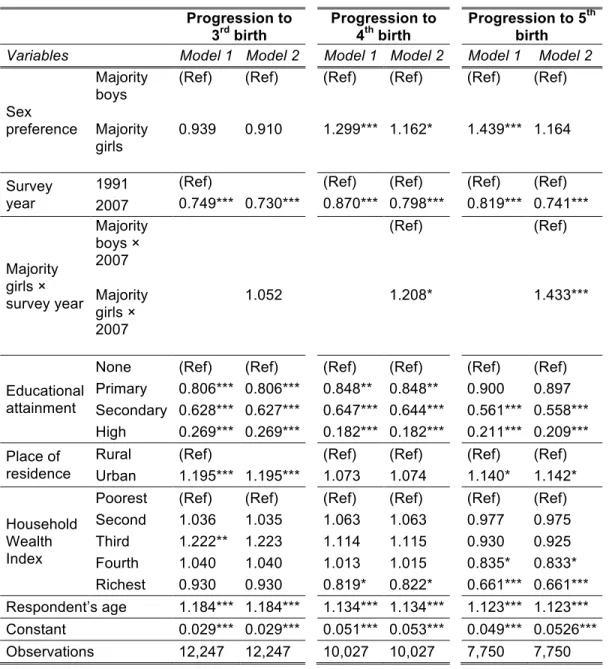
Table 6: Odds ratios for progressing to next birth
Progression to 3rd birth
Progression to 4th birth
Progression to 5th
birth
Variables Model 1 Model 2 Model 1 Model 2 Model 1 Model 2
Sex preference
Majority boys
(Ref) (Ref) (Ref) (Ref) (Ref) (Ref)
Majority girls
0.939 0.910 1.299*** 1.162* 1.439*** 1.164
Survey year
1991 (Ref) (Ref) (Ref) (Ref) (Ref) 2007 0.749*** 0.730*** 0.870*** 0.798*** 0.819*** 0.741***
Majority girls × survey year Majority boys × 2007
(Ref) (Ref)
Majority girls × 2007
1.052 1.208* 1.433***
Educational attainment
None (Ref) (Ref) (Ref) (Ref) (Ref) (Ref) Primary 0.806*** 0.806*** 0.848** 0.848** 0.900 0.897 Secondary 0.628*** 0.627*** 0.647*** 0.644*** 0.561*** 0.558*** High 0.269*** 0.269*** 0.182*** 0.182*** 0.211*** 0.209*** Place of
residence
Rural (Ref) (Ref) (Ref) (Ref) (Ref) Urban 1.195*** 1.195*** 1.073 1.074 1.140* 1.142*
Household Wealth Index
Poorest (Ref) (Ref) (Ref) (Ref) (Ref) (Ref) Second 1.036 1.035 1.063 1.063 0.977 0.975 Third 1.222** 1.223 1.114 1.115 0.930 0.925 Fourth 1.040 1.040 1.013 1.015 0.835* 0.833* Richest 0.930 0.930 0.819* 0.822* 0.661*** 0.661*** Respondent’s age 1.184*** 1.184*** 1.134*** 1.134*** 1.123*** 1.123*** Constant 0.029*** 0.029*** 0.051*** 0.053*** 0.049*** 0.0526*** Observations 12,247 12,247 10,027 10,027 7,750 7,750
23
I ran models that tested for interaction between having majority girls (measure of son preference) and year, respondents’ education and place of residence. However, there was no significant interaction between number of previous sons and respondent’s education or place of residence – the effect of gender composition of previous children did not differ for urban and rural residents or for women with varying education levels. But the effect of son preference on progression to next birth is higher in 2007 than 1991 when progressing from three to four births (at the 90 percent significance level only) and four to five births (model 2s in Table 6).
6.3.2 Current use
If women are using sex preferential stopping behavior to achieve their desired
compositional goals then there should be differentials in contraceptive use by sex composition of previous births. Table 7 shows current use of contraception by gender composition of
previous births for 1991 and 2007. The differentials are as expected; contraceptive use is higher for women with all or majority sons than for women with all or majority daughters. While contraceptive use rates increase substantially over time, the differentials in use are strong for both years. Once again, there is evidence of a slight preference for boys with at least one
24
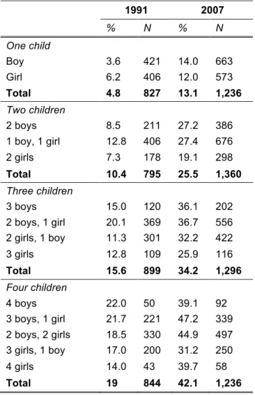
Table 7: Current Use of contraception, by gender composition of children
1991 2007
% N % N
One child
Boy 3.6 421 14.0 663 Girl 6.2 406 12.0 573
Total 4.8 827 13.1 1,236
Two children
2 boys 8.5 211 27.2 386 1 boy, 1 girl 12.8 406 27.4 676 2 girls 7.3 178 19.1 298
Total 10.4 795 25.5 1,360
Three children
3 boys 15.0 120 36.1 202 2 boys, 1 girl 20.1 369 36.7 556 2 girls, 1 boy 11.3 301 32.2 422 3 girls 12.8 109 25.9 116
Total 15.6 899 34.2 1,296
Four children
4 boys 22.0 50 39.1 92 3 boys, 1 girl 21.7 221 47.2 339 2 boys, 2 girls 18.5 330 44.9 497 3 girls, 1 boy 17.0 200 31.2 250 4 girls 14.0 43 39.7 58
Total 19 844 42.1 1,236
The results of the logistic regression analysis in Table 8 show that this differential stopping behavior persists even when controlling for other characteristics. Model 1 shows that the odds of using contraception with only one son or two or more sons are 1.28 (e0.249) and 1.87
(e0.628) times the odds with no sons, when controlling for year, parity, place of residence,
25
Table 8: Logistic regression coefficients for current use of contraception
Variables Model 1 Model 2
Number of sons
0 sons (Ref) (Ref) 1 son 0.249*** 0.0987
(0.0889) (0.164) 2+ sons 0.628*** 0.368** (0.0926) (0.152)
Survey year
1991 (Ref) (Ref)
2007 1.158*** 0.853*** (0.0495) (0.163)
No. of sons × survey year
0 sons × 2007 (ref)
1 son × 2007 0.211
(0.192) 2+ sons × 2007 0.368** (0.172)
Total number of children
One (Ref) (Ref)
Two 0.667*** 0.660*** (0.101) (0.101) Three 1.045*** 1.032***
(0.105) (0.105) Four 1.426*** 1.415***
(0.110) (0.109) Five 1.504*** 1.496***
(0.112) (0.111)
Educational attainment
None (Ref) (Ref)
Primary 0.453*** 0.456*** (0.0659) (0.0660) Secondary 0.736*** 0.739*** (0.0684) (0.0684) High 0.936*** 0.946*** (0.103) (0.103)
Place of residence
Rural (Ref) (Ref)
Urban 0.274*** 0.275*** (0.0523) (0.0524)
Household Wealth Index
Poorest (Ref) (Ref) Second 0.521*** 0.523***
(0.0847) (0.0848) Third 0.834*** 0.838*** (0.0834) (0.0835) Fourth 1.205*** 1.208*** (0.0855) (0.0856) Richest 1.564*** 1.567*** (0.0942) (0.0943)
Respondent’s age -0.00650* (0.00338) -0.00667** (0.00338)
Constant -4.496*** -4.268***
(0.146) (0.183)
Observations 13,836 13,836
26
Similar to progression results, I found an interaction effect between number of previous sons and year (model 2, Table 8): even though women in 2007 were more likely to be using contraception than those in 1991 (e0.853 = odds ratio of 2.3), the effect of having sons (versus having no sons) on the odds of contraceptive use was greater in 2007. These results are in the expected direction – as family size gets smaller, the preference for sons becomes harder to realize and there is greater pressure for preferential behavior.
6.3.3 Intentions
27
Table 9: Intention to have no more children, by gender composition of previous children
1991 2007
% N % N
One child
Boy 6.7 405 10.7 653
Girl 6.1 395 4.9 566
Total 6.4 800 8.0 1,219
Two children
2 boys 23.3 206 33.2 376
1 boy, 1 girl 25.6 383 36.7 660
2 girls 8.3 168 12.2 287
Total 21.1 757 30.4 1,323
Three children
3 boys 38.8 116 58.6 198
2 boys, 1 girl 47.0 349 66.6 539 2 girls, 1 boy 29.6 294 47.1 414
3 girls 21.1 104 18.3 115
Total 36.8 863 54.6 1,266
Four children
4 boys 57.1 49 65.2 89
3 boys, 1 girl 59.5 215 84.1 333 2 boys, 2 girls 57.5 320 82.6 483 3 girls, 1 boy 43.7 192 63.5 241
4 girls 15.0 40 28.6 56
Total 52.7 816 75.4 1,202
This table also demonstrates the overall decrease in desired family size – at all parity levels in 2007, a larger proportion of women intend to stop childbearing than their
28
Table 10: Logistic regression coefficients for intention to stop (have no more) childbearing
Variables Model 1 Model 2
Number of sons
0 sons (Ref) (Ref) 1 son 1.166*** 1.278***
(0.0962) (0.153) 2+ sons 1.846*** 1.278***
(0.0973) (0.146)
Survey year
1991 (Ref) (Ref) 2007 0.887*** 0.134
(0.0485) (0.175)
No. of sons × survey year
0 sons × 2007 (Ref) 1 son × 2007 0.530***
(0.195) 2+ sons × 2007 0.920***
(0.184)
Total number of children
One (Ref) (Ref) Two 1.003*** 0.979***
(0.108) (0.108) Three 1.547*** 1.506***
(0.109) (0.109) Four 2.154*** 2.119***
(0.114) (0.114) Five 2.564*** 2.541***
(0.115) (0.115)
Educational attainment
None (Ref) (Ref) Primary 0.322*** 0.330***
(0.0767) (0.0770) Secondary 0.593*** 0.604*** (0.0822) (0.0822) High 0.232* 0.262**
(0.120) (0.121)
Place of residence
Rural (Ref) (Ref) Urban 0.191*** 0.189***
(0.0572) (0.0574)
Household Wealth Index
Poorest (Ref) (Ref) Second 0.291*** 0.298***
(0.0721) (0.0724) Third 0.409*** 0.416*** (0.0750) (0.0753) Fourth 0.748*** 0.753*** (0.0821) (0.0824) Richest 0.918*** 0.921*** (0.0962) (0.0963)
Respondent’s age 0.0853*** 0.0855*** (0.00365) (0.00365)
Constant -7.023*** (0.172) -6.524*** (0.198)
Observations 13,381 13,381
29
30 CHAPTER 7: DISCUSSION
Son preference serves as an indirect measure of gender discrimination in a society. When fertility falls son preference is more visible and becomes a useful indicator of gender discrimination as well as an important factor affecting contraceptive uptake, fertility levels, and thereby sex ratios. The findings of this paper indicate that in Pakistan evidence of gender discrimination is unmistakable and is playing an increasingly important role in fertility behavior and in altering sex ratios.
Overall, the analysis presented provides strong evidence that women are using selective stopping behavior to achieve their desired compositional goals. Pakistani women are more likely to intend to go on to have another child and/or be a non-user of contraception if they do not have the desired number of sons (one or two). Moreover, the abnormally high SRB for those with no or one son (shown in Table 3) is as Bongaarts says “unambiguous evidence” of sex selective abortion taking place. An abnormal SRB of 110 implies that of the 140 abortions for every 1,000 pregnancies that take place in Pakistan (Vlassoff et al. 2009), 13 percent are sex-selective abortions to achieve desired gender composition (see Table 4 for calculation of the number of sex-selective abortions).
This evidence holds strong implications for future challenges facing Pakistan’s
31
Moreover, differential stopping will intensify gender inequality because girls will belong to larger households disproportionately because families with girls are the ones that continue childbearing until a son is born. The reduction in resources available to each child in larger families will thus affect girls more.
The results of this paper are relevant not only for Pakistan’s future but also for other patriarchal societies, especially those currently experiencing fertility declines. The strong evidence of skewed sex ratios at birth suggests that lack of legal and safe abortion services are not sufficient in protecting against the practice of sex-selective abortions. Patriarchal
32 REFERENCES
Arnold, Fred, Sunita Kishor, and T. K. Roy. 2002. “Sex-Selective Abortions in India.” Population and Development Review 28(4): 759–85. doi: 10.1111/j.1728-4457.2002.00759.x.
Bharadwaj, Prashant and Leah K. Lakdawala. 2013. “Discrimination Begins in the Womb:
Evidence of Sex-Selective Prenatal Investments.” Journal of Human Resources 48:71–113.
Bongaarts, John and Robert G. Potter. 1983. Fertility, Biology, and Behavior: An Analysis of the Proximate Determinants. New York: Academic Press.
Bongaarts, John B. 2013. “Implementation for Preferences for Male Offspring.” Population and Development Review 39(2): 185–208. doi: 10.1111/j.1728-4457.2013.00588.x.
Das Gupta, Monica and P. N. Mari Bhat. 1997. “Fertility Decline and Increased Manifestation of Sex Bias in India.” Population Studies 51(3): 307–15. Retrieved November 12, 2013 (http://www.jstor.org/stable/2952474).
Davis, Kingsley and Judith Blake. 1956. “Social Structure and Fertility: An Analytic Framework.” Economic Development and Cultural Change 4(3): 211–35. Retrieved November 12, 2013 (http://www.jstor.org/stable/1151774).
Duthé, Géraldine, France Meslé, Jacques Vallin, Irina Badurashvili, and Karine Kuyumjyan. 2012. “High Sex Ratios at Birth in the Caucasus: Modern Technology to Satisfy Old Desires.” Population and Development Review 38(3): 487–501. doi:
10.1111/j.1728-4457.2012.00513.x.
Dyson, Tim. 2012. “Causes and Consequences of Skewed Sex Ratios.” Annual Review of Sociology 38: 443–61. Retrieved November 12, 2013
(http://www.annualreviews.org/doi/abs/10.1146/annurev-soc-071811-145429).
Ebenstein, Avraham Y. 2007. “Fertility Choices and Sex Selection in Asia: Analysis and Policy.” Working Paper. Social Science Research Network (SSRN), Rochester, NY. Retrieved November 12, 2013 (http://papers.ssrn.com/sol3/papers.cfm?abstract_id=965551).
Filmer, Deon, Jed Arnold Friedman, and Norbert Schady. 2009. “Development, Modernization, and Childbearing: The Role of Family Sex Composition.” World Bank Economic Review 23(3): 371–98. doi: 10.1093/wber/lhp009.
Garenne, Michel. 2008. “Situations of Fertility Stall in Sub-Saharan Africa.” African Population Studies 23(2): 173–88. Retrieved November 12, 2013
33
Guilmoto, Christophe Z. 2007. “Characteristics of Sex Ratio Imbalance in India and Future Scenarios.” Paper presented at the Fourth Asia and Pacific Conference on Sexual and Reproductive Health and Rights, October, Hyderabad, India. Retrieved November 12, 2013 (http://www.unfpa.org/gender/docs/studies/india.pdf).
---. 2009. “The Sex Ratio Transition in Asia.” Population and Development Review 35(3): 519– 549. doi: 10.1111/j.1728-4457.2009.00295.x.
---. 2012. “Son Preference, Sex Selection, and Kinship in Vietnam.” Population and Development Review 38(1): 31–54. doi: 10.1111/j.1728-4457.2012.00471.x.
Hesketh, Therese and Zhu Wei Xing. 2006. “Abnormal Sex Ratios in Human Populations: Causes and Consequences.” Proceedings of the National Academy of Sciences of the United States of America 103(36): 13271–5. Retrieved November 12, 2013
(http://www.pnas.org/content/103/36/13271.full).
Kulkarni, P. M. 2007. “Estimation of Missing Girls at Birth and Juvenile Ages in India.”United Nations Population Fund (UNFPA)-India, New Delhi, India. Retrieved November 12, 2013 (http://india.unfpa.org/drive/MissingGirlsatBirthpaper-August2007Kulkarni.pdf).
National Institute of Population Studies (NIPS) (Pakistan) and Macro International Inc. 2008. Pakistan Demographic and Health Survey 2006–07. Islamabad: National Institute of Population Studies and Macro International Inc. Retrieved November 12, 2013 (http://www.measuredhs.com/pubs/pdf/FR200/FR200.pdf).
---. 2013. Pakistan Demographic and Health Survey 2012–13 Preliminary Report. Islamabad: National Institute of Population Studies and Macro International Inc. Retrieved
November 12, 2013 (http://www.measuredhs.com/pubs/pdf/PR35/PR35.pdf).
Pollard, Michael S. and S. Philip Morgan. 2002. “Emerging Parental Gender Indifference? Sex Composition of Children and the Third Birth.” American Sociological Review 67(4): 600– 13. Retrieved November 12, 2013 (http://www.jstor.org/stable/3088947).
Sathar, Zeba A. and John B. Casterline. 1998. “The Onset of Fertility Transition in Pakistan.” Population and Development Review 24(4): 773–96. Retrieved November 12, 2013 (http://www.popcouncil.org/pdfs/councilarticles/pdr/PDR244Sathar.pdf).
Sathar, Zeba A., Susheela Singh, and Fariyal F. Fikree. 2007. “Estimating the Incidence of Abortion in Pakistan.” Studies in Family Planning 38(1): 11–22. Retrieved November 12, 2013 (http://www.jstor.org/stable/20454380).
34
ST/ESA/SER.A/313. Retrieved November 12, 2013
(http://esa.un.org/wpp/Documentation/pdf/WPP2010_Volume-I_Comprehensive-Tables.pdf).
Vlassoff, Michael, Susheela Singh, and Gustavo Suarez. 2009. Abortion in Pakistan. In Brief No. 2. New York: Guttmacher Institute. Retrieved November 12, 2013
(http://www.guttmacher.org/pubs/IB_Abortion-in-Pakistan.pdf).
Zaidi, Batool, Zeba Sathar, Minhaj ul Haque, and Fareeha Zafar. 2012. The Power of Girls’ Schooling for Young Women’s Empowerment and Reproductive Health. Islamabad: Population Council. Retrieved November 12, 2013