EQUITY RISK PREMIUM: EXPECTATIONS GREAT

AND

S

MALL

Richard A. Derrig* and Elisha D. Orr

A

The equity risk premium (ERP) is an essential building block of the market value of risk. In theory, the collective action of all investors results in an equilibrium expectation for the return on the market portfolio excess of the risk-free return, the ERP. The ability of the valuation actuary to choose a sensible value for the ERP, whether as a required input to capital asset pricing model valuation, or any of its descendants, is as important as choosing risk-free rates and risk relatives (betas) to the ERP for the asset at hand.

The historical realized ERP for the stock market appears to be at odds with pricing theory parameters for risk aversion. Since 1985, there has been a constant stream of research, each of which reviews theories of estimating market returns, examines historical data periods, or both. Those ERP value estimates varywidelyfrom about ⫺1% to about 9%, based on a geometric or arithmetic averaging, short or long horizons, short- or long-run expectations, unconditional or conditional distributions, domestic or international data, data periods, and real or nominal returns. This paper examines the principal strains of the recent research on the ERP and catalogues the empirical values of the ERP implied by that research. In addition, the paper supplies several time series analyses of the standard Ibbotson Associates 1926 –2002 ERP data using short Treasuries for the risk-free rate. Recommendations for ERP values to use in common actuarial valuation problems also are offered.

“What I actually think is that our prey, called the equity risk premium, is extremely elusive.”

—Stephen A. Ross (2002, p. 22)

1. I

The equity risk premium (ERP) is an essential building block of the market value of risk. In theory, the collective action of all investors re-sults in an equilibrium expectation for the return on the market portfolio excess of the risk-free return, the ERP. The ability of the valuation ac-tuary to choose a sensible value for the ERP— whether as a required input to capital asset pric-ing model (CAPM) valuation or any of its descendants1—is as important as choosing

risk-free rates and risk relatives (betas) to the ERP for the asset at hand. Risky discount rates, asset allocation models, and project costs of capital are common actuarial uses of ERP as a benchmark rate. The ERP should be of particular interest to actu-aries. For pensions and annuities backed by bonds and stocks, the actuary needs to have an under-standing of the ERP and its variability compared to fixed-horizon bonds. Variable products, including guaranteed minimum death benefits, require accu-rate projections of returns to ensure adequate fu-ture assets. With the latest research producing a relatively low ERP, the rationale for including equi-ties in insurers’ asset holdings is being tested.

In describing individual investment account guarantees, LaChance and Mitchell (2003) point out an underlying assumption of pension asset investing that, based only on the historical record, future equity returns will continue to out-perform bonds; they clarify that those higher ex-* Richard A. Derrig is Senior Vice President, Automobile Insurers

Bureau of Massachusetts, 101 Arch Street, Boston, MA 02110, e-mail: [email protected].

†

Elisha D. Orr is a Research Assistant, Automobile Insurers Bureau of Massachusetts, 101 Arch Street, Boston, MA 02110, e-mail: [email protected].

1

The multifactor arbitrage pricing theory of Ross (1976), the three-factor model of Fama and French (1992) and the recent Mamaysky

(2002) five-factor model for stocks and bonds are all examples of enhanced CAPM models.

pected equity returns come with the additional higher risk of equity returns. Ralfe et al. (2003) support the risky equity view and discuss their pension experience with an all-bond portfolio. Recent projections in some literature of a zero or negative ERP challenge the assumptions underly-ing these views.

By reviewing some of the most recent and rel-evant work on the issue of the ERP, actuaries will have a better understanding of how these values were estimated, critical assumptions that allowed for such a low ERP, and the time period for the projection (see Appendix B). Actuaries can then make informed decisions for expected investment results going forward.

In 1985, Mehra and Prescott published their work on theequity risk premium puzzle: the fact that the historical realized ERP for the stock mar-ket from 1889 –1978 appeared to be at odds with and, relative to Treasury bills, far in excess of asset pricing theory values based on investors with reasonable risk aversion parameters. Since then, there has been a constant stream of re-search, each of which reviews theories of estimat-ing market returns, examines historical data pe-riods, or both (for example, see Cochrane 1997, Cornell 1999, or Equity Risk Premium Forum 2002). Those ERP value estimates vary widely, from about⫺1% to about 9%, based on geometric or arithmetic averaging, short or long horizons, short-or long-run means, unconditional short-or conditional expectations, using domestic or international data, differing data periods, and real or nominal returns. Brealey and Myers (2000), in the sixth edition of their standard corporate finance text-book, believe a range of 6 – 8.5% for the U.S. ERP is reasonable for practical project valuation. Is that a fair estimate?

Current research on the ERP is plentiful. This paper covers a selection of mainstream articles and books that describe different approaches to estimating theex ante ERP. We select examples of the research that cover the most important approaches to the ERP. We begin by describing the methodology of using historical returns to predict future estimates. We identify the many varieties of ERPs in order to alert the reader to the fact that numerical estimates of the ERP that appear different may instead be about the same under a common definition. We examine the well-known Ibbotson Associates 1926 –2002 data

se-ries for stationarity, that is, time invariance of the mean ERP. We show by several statistical tests that stationarity cannot be rejected and the best estimate going forward, ceteris paribus, is the realized mean. This paper will examine the prin-cipal strains of the recent research on the ERP and catalogue the empirical values of the ERP implied by that research (see Appendix B).

We first discuss how the Social Security Admin-istration derives estimates of the ERP. Then, we survey the puzzle research, that is, the literature written in response to the equity premium puzzle suggested by Mehra and Prescott (1985). We cover five major approaches from the literature. Next, we report from two surveys of “experts” on the ERP. Finally, after describing the main strains of research, we explore some of the implications for practicing actuaries.

We do not discuss the important companion problem of estimating the risk relationship of an individual company, line of insurance, or project with the overall market. Within a CAPM or Fama-French framework, the problem is estimating a market beta.2 _{Actuaries should be aware,}

how-ever, that simple 60-month regression betas are biased low where size or nonsynchronous trading is a substantial factor (Kaplan and Peterson 1998, Pratt 1998, p. 86). Adjustments are made to his-torical betas in order to remove the bias and derive more accurate estimates. Elton and Gru-ber (1995, p. 148) explain that by testing the relationship of beta estimates over time, empiri-cal studies have shown that an adjustment toward the mean should be made to project future betas.

2. T

E

R

P

Based on the definition in Brealey and Myers (2000), the ERP is the “expected additional re-turn for making a risky investment rather than a safe one” (p. 1071). In other words, the ERP is the difference between the market return and a risk-free return. Market returns include both divi-dends and capital gains. Because both the histor-ical ERP and the prospective ERP have been

2_{According to CAPM, investors are compensated only for}

nondiver-sifiable, or market, risk. The market beta becomes the measurement of the extent to which returns on an individual security co-vary with the market. The market beta times the ERP represents the nondiver-sifiable expected return from an individual security.

referred to simply as the ERP, the terms ex post and ex ante are used to differentiate between them but are often omitted. Table 1 shows the historical annual average returns from 1926 to 2002 for large company equities (S&P 500), Treasury bills and bonds, and their arithmetic differences using data from Ibbotson Associates (2003a,b); the entire series is shown in Appendix A.

In 1985, Mehra and Prescott introduced the idea of the ERP puzzle. The puzzling result is that the historical realized ERP for the stock market using 1889 –1978 data appeared to be at odds with and, relative to Treasury bills, far in excess of asset pricing theory values based on normal parametrizations of risk aversion. When using standard frictionless return models and historical growth rates in consumption, the real risk-free rate, and the ERP, the resulting relative risk aver-sion parameter appears too high. By choosing a maximum relative risk aversion parameter to be 10 and using the growth in consumption, Mehra and Prescott’s model produces an ERP much lower than the historical premium.3

Their result inspired a stream of finance liter-ature that attempts to solve the puzzle. Two dif-ferent research threads have emerged. One thread, including behavioral finance, attempts to explain the historical returns with new models and different assumptions about investors (see, e.g., Benartzi and Thaler 1995 and Mehra 2002). A second thread is from a group that provides estimates of the ERP that are derived from his-torical data and/or standard economic models. Some in this latter group argue that historical returns may have been higher than those that should be required in the future. In a curiously asymmetric way, there are no serious studies yet concluding that the historical results are too low to serve asex ante estimates.

Although both groups have made substantial and provocative contributions, the behavioral models do not give any ex ante ERP estimates other than explaining and supporting the histor-ical returns. We presume, until results show oth-erwise, that the behaviorists support the histori-cal average as theex anteunconditional long-run

expectation. Therefore, we focus on the latter to catalogue ERP estimates other than those based on the historical approach,4 but we will discuss both as important strains for puzzle research.

3. ERP T

Many different types of ERP estimates can be given, even though they are labeled by the same general term. These estimates vary widely; cur-rently the estimates range from about 9% to a small negative. When ERP estimates are given, one should determine the type before comparing to other estimates. Here are seven important types to look for when given an ERP estimate:

● Geometric versus arithmetic averaging.

● Short versus long investment horizon.

● Short- versus long-run expectation.

● Unconditional versus conditional on some re-lated variable.

● Domestic United States versus international market data.

● Data sources and periods.

● Real versus nominal returns.

The average market return and ERP can be stated as a geometric or arithmetic mean return. Anarithmetic mean returnis a simple average of a series of returns. Thegeometric mean returnis the compound rate of return; it is a measure of the actual average performance of a portfolio over a given time period. Arithmetic returns are the same or higher than geometric returns, so it is not appropriate to make a direct comparison between an arithmetic estimate and a geometric estimate. However, those two returns can be transformed one to the other. For example, arithmetic returns

3_{Campbell, Lo, and MacKinlay (1997, pp. 307–308) performed a}

similar analysis and found a risk-aversion coefficient of 19, larger than

the reasonable level suggested in Mehra and Prescott’s paper. 4_{See Appendix C.}

Table 1

U.S. Equity Risk Premia 1926 –2002 Annual Equity Returns and Premia versus Treasury Bills,

Intermediate, and Long-Term Bonds

Horizon Equity Returns Risk-Free Return ERP Short 12.20% 3.83% 8.37% Intermediate 12.20 4.81 7.40 Long 12.20 5.23 6.97

Source: Authors’ calculations using Ibbotson Associates (2003a, p. 38 –39, 177, 238 –39, 246 – 47).

can be approximated from geometric returns by the formula

AR⫽GR⫹␴

2

2, ␴

2 _{the variance of the}

(arithmetic) return process (see Welch 2000, Dimson et al. 2002, and Ibbot-son and Chen 2003). Arithmetic averages of pe-riodic returns are to be preferred when estimating next period returns since they, not geometric averages, reproduce the proper probabilities and means of expected returns.5 ERPs can be gener-ated by arithmetic differences (Equity ⫺ Risk Free) or by geometric differences ([(1⫹Equity)/ (1⫹Risk Free)]⫺1). Usually, the arithmetic and geometric differences produce similar estimates.6 A second important difference in ERP estimate types is the horizon. Thehorizonindicates the total investment or planning period under consideration. For estimation purposes, the horizon relates to the term or maturity of the risk-free instrument that is used to determine the ERP. Ibbotson Associates (2003a, p. 177) provides definitions for three differ-ent horizons. The short-horizon expected ERP is defined as “the large company stock total returns minus U.S. Treasury bill total returns.” Note, the income return and total return are the same for U.S. Treasury bills. Theintermediate-horizon expected ERP is “the large company stock total returns mi-nus intermediate-term government bond income returns.” Finally, thelong-horizonexpected ERP is “the large company stock total returns minus long-term government bond incomereturns.” (Table 1 displays the short-horizon ERP.)

For the Ibbotson data, Treasury bills have a maturity of approximately one month, intermedi-ate-term government bonds have a maturity around five years, and long-term government bonds have a maturity of about 20 years. Although the Ibbotson definitions may not apply to other research, we will classify ERP estimates based on these guidelines to establish some consistency among the current re-search. The reader should note that Ibbotson Asso-ciates recommends the income return (or the yield)

when using a bond as the risk-free rate rather than the total return.7

A third type is the length of time of the ERP forecast. We distinguish between short-run and long-run expectations.Short-runexpectations re-fer to the current ERP or, for this paper, a pre-diction of up to 10 years. In contrast, the long-run expectation is a forecast over 10 years to as many as 75 years for social security purposes. Ten years appears an appropriate breaking point based on the current literature surveyed.

The next difference is whether the ERP esti-mate is unconditional or conditionedon one or more related variables. In defining this type, we refer to an admonition by Constantinides (2002) of the differences in these estimates:

“First, I draw a sharp distinction between condi-tional, short-term forecasts of the mean equity return and premium andestimates of the uncon-ditional mean.I argue that the currently low con-ditional short-term forecasts of the return and premium do not lessen the burden on economic theory to explain the large unconditional mean equity return and premium, as measured by their sample average over the past one hundred and thirty years” (p. 1568).

Many of the estimates we catalogue below will be conditional ones, conditional on dividend yield, expected earnings, capital gains, or other assump-tions about the future.

ERP estimates can also exhibit aU.S. versus in-ternational market type depending on the data used for estimation purposes and the ERP being estimated. Dimson et al. (2002) notes that, at the start of 2000, the U.S. equity market, while domi-nant, was slightly less than one-half (46.1%) of the total international market for equities, capitalized at $52.7 trillion. Table 2 shows a comparison of historical ERP values for the United States and the world. Data from the non-U.S. equity markets are clearly different from those of U.S. markets and, hence, will produce different estimates for returns

5_{For a complete discussion of the arithmetic/geometric choice, see}

Ibbotson Associates (2003b, pp. 71–3). See also Dimson et al. (2002, p. 35), and Brennan and Schwartz (1985).

6

The arithmetic difference is the geometric difference multiplied by 1⫹Risk Free.

7_{The reason for this is two-fold. First, when issued, the yield is the}

expected market return for the entire horizon of the bond. No net capital gains are expected for the market return for the entire horizon of the bond. No capital gains are expected at the default-free matu-rity. Second, historical annual capital gains on long-term government bonds average near zero (0.4%) over the 1926 –2002 period (Ibbot-son Associates 2003a, tables 6 –7).

and ERP.8Results for the entire world equity mar-ket will, of course, be a weighted average of the U.S. and non-U.S. estimates.

The next type is thedata source and periodused for the market and ERP estimates. Whether given an historical average of the ERP or an estimate from a model using various historical data, the ERP esti-mate will be influenced by the length, timing, and source of the underlying data used. The time series compilations are primarily annual or monthly re-turns. Occasionally, daily returns are analyzed, but not for the purpose of estimating an ERP. Some researchers use as much as 200 years of history; the Ibbotson data currently uses S&P 500 returns from 1926 to the present.9

As an example, Siegel (2002) examined a series of real U.S. returns beginning in 1802.10 He used three sources to obtain the data. For the first period, 1802–1870, characterized by stocks of financial or-ganizations involved in banking and insurance, he cites Schwert (1990). The second period, 1871– 1925, incorporates Cowles stock indexes compiled in Shiller (1989). The last period, beginning in 1926, uses data from the Center for Research in Security Prices (CRSP), University of Chicago Graduate School of Business; these are the same data underlying Ibbotson Associates calculations.

Goetzmann et al. (2001) constructed an NYSE data series for 1815–1925 to add to the 1926 – 1999 Ibbotson series. They concluded that the pre-1926 and post-1926 data periods show differ-ences in both risk and reward characteristics. They highlighted the fact that inclusion of pre-1926 data will generally produce lower estimates of ERPs than relying exclusively on the Ibbotson post-1926 data, similar to that shown in Appendix A. Several studies that rely on pre-1926 data, catalogued in Appendix B, show the magnitudes of these lower estimates.11 Table 3 displays

Sie-gel’s ERPs for three subperiods. He notes that subperiod III, 1926 –2001, shows a larger ERP (4.7%), or a smaller real risk-free mean (2.2%), than the prior subperiods.12

Smaller subperiods will show much larger vari-ations in equity, bill, and ERP returns. Table 4 displays the Ibbotson returns and short-horizon risk premia for subperiods as small as five years. The scatter of results is indicative of the under-lying large variation (20% std dev) in annual data. In calculating an expected equity risk premium by averaging historical data, projecting historical data using growth models, or even conducting a survey, one must determine a proxy for the “mar-ket.” Common proxies for the U.S. market include the S&P 500, the NYSE index, and the NYSE, AMEX, and NASDAQ index (Ibbotson Associates 2003b, p. 92). For the purpose of this paper, we use the S&P 500 and its antecedents as the market. However, in the various research surveyed, many different market proxies were assumed. We have already discussed using international versus ERP domestic data when describing different MRP types. With international data, different proxies for other country, region, or world markets are used. For example, Dimson (2002) and Claus and Thomas (2001) use international market data.

8_{One qualitative difference can arise from the collapse of equity}

markets during war time.

9_{For the Ibbotson analysis of the small stock premium, the NYSE/}

AMEX/NASDAQ combined data are used, with the S&P 500 data falling within deciles 1 and 2 (Ibbotson Associates 2003b, pp. 66 and Chapter 7.)

10_{A more recent alternative is Wilson and Jones (2002), as cited by}

Dimson et al. (2002, p. 39).

11_{Using Wilson and Jones’ 1871–2002 data series, time series}

anal-yses show no significant ERP difference between the 1871–1925 period and the 1926 –2002 period; one cannot distinguish the old

from the new. The overall average is lower with the additional 1871–1925 data, but on a statistical basis, they are not significantly different. Assuming the equivalency of the two data series for 1871– 1925 (Goetzmann et al. 2001 and Wilson and Jones 2002), the risk difference found by Goetzmann et al. must be determined by a significantly different ERP in the pre-1871 data. The 1871–1913 return that is prior to personal income tax and that appears to be about 35% lower than the 1926 –2002 period average of 11.8%, might simply reflect a zero valuation for income taxes in the pre-1914 returns. Adjusting the pre-1914 data for taxes would most likely make the ERP for the entire period (1871–2002) approximately equal to 7.5%, the 1926 –2002 average.

12

The low risk-free return is indicative of the “risk-free rate puzzle,” the twin of the ERP puzzle. For details see Weil (1989).

Table 2

Worldwide Equity Risk Premia, 1900 –2000 Annual Equity Risk Premium Relative to

Treasury Bills

Country Geometric Mean Arithmetic Mean

United States 5.8% 7.7%

World 4.9 6.2

For domestic data, different proxies have been used over time as stock market exchanges have expanded. (For a data series that is a mixture of the NYSE exchange, NYSE, AMEX, and NASDAQ stock exchange, and the Wilshire 5000, see Dim-son 2002, p. 306.) Fortunately, as shown by Ib-botson Associates (2003b), the issue of a U.S. market proxy does not have a large effect on the ERP estimate because the various indices are highly correlated. For example, the S&P 500 and the NYSE have a correlation of 0.95, the S&P 500

and NYSE/AMEX/NASDAQ 0.97, and the NYSE and NYSE/AMEX/NASDAQ 0.90 (Ibbotson Associ-ates 2003b, p. 93, using data from October 1997– September 2002). Therefore, the equity proxy selected is one reason for slight differences in the estimates of the market risk premium.

As a final note, stock returns and risk-free rates can be stated innominal orrealterms. Nominal includes inflation; real removes inflation. The ERP should not be affected by inflation because either the stock return and risk-free rate both Table 3

Short-Horizon Equity Risk Premium by Subperiods

Subperiod I Subperiod II Subperiod III

1802–1870 1871–1925 1926–2001

Real Geometric Stock Returns 7.0% 6.6% 6.9%

Real Geometric Long-Term Governments 4.8 3.7 2.2

Equity Risk Premium 2.2 2.9 4.7

Source:Siegel (2002, pp. 13 and 15).

Table 4

Average Short-Horizon Risk Premium over Various Time Period

Year

Common stocks U.S. Treasury Bills Short-Horizon

Total Annual Returns Total Annual Returns Risk Premium

All Data 1926–2002 12.20% 3.83% 8.37% 50-year 1953–2002 12.50 5.33 7.17 40-year 1963–2002 11.80 6.11 5.68 30-year 1943–1972 14.55 2.54 12.02 1973–2002 12.21 6.61 5.60 15-year 1928–1942 5.84 0.95 4.89 1943–1957 17.14 1.20 15.94 1958–1972 11.96 3.87 8.09 1973–1987 11.42 8.20 3.22 1988–2002 13.00 5.03 7.97 10-year 1933–1942 12.88 0.15 12.73 1943–1952 17.81 0.81 17.00 1953–1962 15.29 2.19 13.11 1963–1972 10.55 4.61 5.94 1973–1982 8.67 8.50 0.17 1983–1992 16.80 6.96 9.84 1993–2002 11.17 4.38 6.79 5-year 1928–1932 ⫺8.25 2.55 ⫺10.80 1933–1937 19.82 0.22 19.60 1938–1942 5.94 0.07 5.87 1943–1947 15.95 0.37 15.57 1948–1952 19.68 1.25 18.43 1953–1957 15.79 1.97 13.82 1958–1962 14.79 2.40 12.39 1963–1967 13.13 3.91 9.22 1968–1972 7.97 5.31 2.66 1973–1977 2.55 6.19 ⫺3.64 1978–1982 14.78 10.81 3.97 1983–1987 16.93 7.60 9.33 1988–1992 16.67 6.33 10.34 1993–1997 21.03 4.57 16.46 1998–2002 1.31 4.18 ⫺2.88

include the effects of inflation (both stated in nominal terms) or neither have inflation (both stated in real terms). If both returns are nominal, the difference in the returns is generally assumed to remove inflation. Otherwise, both terms are real, so inflation is removed prior to finding the ERP. While numerical differences in the real and nominal approaches may exist, their magnitudes are expected to be small.

4. E

R

P

1926 –2002

As an example of the importance of knowing the types of ERP estimates under consideration, Ta-ble 5 displays ERP returns that each use the same historical data, but are based on arithmetic or geometric returns and the type of horizon. The ERP estimates are quite different.13

5. H

M

The historical methodology uses averages of past returns to forecast future returns. Different time periods may be selected, but the two most com-mon periods arise from data provided by either Ibbotson or Siegel. The Ibbotson series begins in 1926 and is updated each year. The Siegel series begins in 1802, with the most recent compilation using returns through 2001.

Appendix A provides ERP estimates using Ib-botson data for the 1926 –2002 period that we use

in this paper for most illustrations. We begin with a look at the ERP history through a time series analysis of the Ibbotson data.

6. T

S

A

Much of the analysis addressing the ERP puzzle relies on the annual time series of market, risk-free and risk premium returns. Two opposite views can be taken of these data. One view would have the 1926 –2002 Ibbotson data or the 1802– 2001 Siegel data represent one data point; that is, we have observed one path for the ERP through time from the many possible 77- or 200-year paths. This view rests upon the existence or as-sumption of a stochastic process with (possibly) intertemporal correlations.

While mathematically sophisticated, this model is particularly unhelpful without some testable hint at the details of the generating stochastic process. The practical view is that the observed returns are random samples from annual distributions that are i.i.d. (independent and identically distributed) about the mean. The obvious advantage is that we have at hand 77 or 200 observations on the i.i.d. process to analyze. We adopt the latter view.

Some analyses adopt the assumption of station-arity of ERP; that is, the true mean does not change with time. Figure 1 displays the Ibbotson ERP data and highlights two subperiods, 1926 – 1959 and 1960 –2002.14 While the mean ERP for

13_{The nominal and real ERPs are identical in Table 5 because the ERPs}

are calculated as arithmetic differences, and the same value of infla-tion will reduce the market return and the risk-free return equally. Geometric differences would produce minimally different estimates for the same types.

14

The ERP shown here are the geometric differences (calculated) rather than the simple arithmetic differences in Table 1; i.e., ERP⫽ [(1⫹rm)/(1⫹rf)]⫺1. The test results are qualitatively the same for

the arithmetic differences. Table 5

ERP Using Same Historical Data (1926 –2002)

RFR Description ERP Description ERP Historical Return

Short nominal Arithmetic short-horizon 8.4%

Short nominal Geometric short-horizon 6.4

Short real Arithmetic short-horizon 8.4

Short real Geometric short-horizon 6.4

Intermediate nominal Arithmetic inter-horizon 7.4 Intermediate nominal Geometric inter-horizon 5.4

Intermediate real Arithmetic inter-horizon 7.4

Intermediate real Geometric inter-horizon 5.4

Long nominal Arithmetic long-horizon 7.0

Long nominal Geometric long-horizon 5.0

Long real Arithmetic long-horizon 7.0

Long real Geometric long-horizon 5.0

the two subperiods appear quite different (11.82% versus 5.27%), the large variance of the process (20.24% std dev) should make them indistinguish-able, statistically speaking.

7. T-T

The standard t-test can be used for the null hy-pothesis H_o: mean 1960 –2002 ⫽ 8.17%, the 77-year mean.15The outcome of the test is shown in Table 6; the null hypothesis cannot be rejected. Another t-test can be used to test whether the subperiod means are different in the presence of unequal variances.16The result is similar to Table 6 and the difference of subperiod means equal to zero cannot be rejected.17

8. T

T

The supposition of stationarity of the ERP series can be supported by ANOVA regressions. The results of regressing the ERP series on time is shown in Table 7. There are no significant time trends in the Ibbotson ERP data.18

9. ARIMA M

Time series analysis using the well-established Box-Jenkins approach can be used to predict future series values through the lag correlation structure (see Harvey 1990, p. 30). The SAS ARIMA proce-dure applied to the full 77 time series data shows: 1. No significant autocorrelation lags.

2. An identification of the series as white noise. 3. ARIMA projection of year 78 ⫹ ERP is 8.17%,

the 77 year average.

All of the above single time series tests point to the reasonability of the stationarity assumption for (at least) the Ibbotson ERP 77-year series.19

10. S

S

A

In the current debate on whether to allow private accounts that may invest in equities, the Office of the Chief Actuary (OCACT) of the Social Security Administration (SSA) has selected certain as-sumptions to assess various proposals (Goss 2001). The relevant selection is to use 7% as the real (geometric) annual rate of return for equities (compare Table 3, subperiod III). This assump-tion is based on the historical return of the 20th century. SSA received further support that showed the historical return for the last 200 years is consistent with this estimate, along with the Ibbotson series beginning in 1926.

For SSA, the calculation of the ERP uses a long-run real yield on Treasury bonds as the risk-free rate. From the assumptions in the 1995 Trustees Report, the long-run real yield on Trea-sury bonds that the Advisory Council proposals

15_{Standard statistical procedures in SAS 8.1 have been used for all}

tests.

16_{Equality of variances is rejected at the 1% level by an F test (F⫽}

2.39, DF⫽33,42).

17_{T-value 1.35, PR⬎兩T兩⫽0.1850 (Cochran method).} 18

The result is confirmed by a separate Chow test on the two subperiods.

19

The same tests applied to the Wilson and Jones 1871–2002 data series show similar results: Neither the 1871–1925 period nor the 1926 –2002 period is different from the overall 1871–2002 period. The overall period and subperiods also show no trends over time. Figure 1

Short-Horizon Equity Risk Premium

Source:Authors’ calculations using Ibbotson Associates (2003a, p. 38 –39), geometric differences.

Table 6

T-Test under the Null Hypothesis That ERP

(1960 –2002) ⴝERP (1926 –2002)ⴝ 8.17% Sample mean 1960–2002 5.27% Sample s.d. 1960–2002 15.83% T-value (DF⫽42) ⫺1.20 PR⬎兩T兩 0.2374 Confidence Interval 95% (0.0040, 0.1014) Confidence Interval 90% (0.0121, 0.0933)

use is 2.3%. Using a future Treasury securities real yield of 2.3% produces a geometric ERP of 4.7% over long-term Treasury securities. More re-cently, the Treasury securities assumption has increased to 3% (Social Security Trustees Report 1999), yielding a 4% geometric ERP over long-term Treasury securities.

At the request of the OCACT, John Campbell, Peter Diamond, and John Shoven were engaged to give their expert opinions on the assumptions Social Security made. Each economist begins with the Social Security assumptions and then explains any difference he or she feels would be more appropriate.

Campbell (2001) considered valuation ratios as a comparison to the returns from the historical approach. The current valuation ratios are at un-usual levels, with a low dividend-price ratio and high price-earnings ratio. He reasoned that the prices are what have dramatically changed these ratios. Campbell presented two views as to the effect of valuation ratios in their current state. One is that valuations will remain at the current level, suggesting much lower expected returns. The second view is a correction to the ratios, resulting in less favorable returns until the ratios readjust. He decided to give some weight to both possibilities, so he lowered the geometric equity return estimate to 5–5.5% from 7%. For the risk-free rate, he used the yield on the long-term in-flation-indexed bonds of 3.5% or the OCACT as-sumption of 3% (see discussion of current yields on Treasury Inflation Protection Securities (TIPS) in Section 16 below). Therefore, his geometric eq-uity premium estimate was around 1.5–2.5%.

Diamond (1999, 2001) used the Gordon growth formula to calculate an estimate of the equity return. The classic Gordon dividend growth model (Brealey and Myers 2000, p. 67) follows.

K⫽共D1/P0兲⫹g

K⫽Expected return or discount rate

P0⫽Price this period

D₁⫽Expected dividend next period

g⫽Expected growth in dividends in perpetuity Based on analysis, he felt that the equity return assumption of 7% for the next 75 years is not consistent with a reasonable level of stock value compared to GDP. Even when increasing the GDP growth assumption, he still did not feel that the equity return was plausible. By reasoning that the next decade of returns will be lower than normal, only then is the equity return beyond that time frame consistent with the historical return. By considering the next 75 years together, he would lower the overall projected equity return to 6 – 6.5%. He argued that the stock market is over-valued, and a correction is required before the long-run historical return is a reasonable projec-tion for the future. By using the OCACT assump-tion of 3% for the long-term real yield on Treasury bonds, Diamond estimated a geometric ERP of about 3–3.5%.

Shoven (2001) began by explaining why the traditional Gordon growth model is not appropri-ate and suggested a modernized Gordon model that allows share repurchases to be included, in-stead of only using the dividend yield and growth rate. By assuming a long-term price-earnings ra-tio between its current and historical value, he came up with an estimate for the long-term real equity return of 6.125%. Using his general esti-mate of 6 – 6.5% for the equity return and the OCACT assumptions for the long-term bond yield, he projected a long-term ERP of approxi-mately 3–3.5%.

All the SSA experts begin by accepting the long-run historical ERP analyses and then modifying that by changes in the risk-free rate or by de-creases in the long-term ERP based on their own personal assessments. We now turn to the major strains in ERP puzzle research.

11. ERP P

R

Campbell and Shiller (2001) began with the as-sumption of mean reversion of dividend/price and price/earnings ratios. Next, they explained the result of prior research (Campbell and Shiller 1988) that found that the dividend-price ratio predicts future prices, and historically, the price Table 7

ERP ANOVA Regressions on Time

Period Time Coefficient P-Value

1926–1959 0.004 0.355

1960–2002 0.001 0.749

corrects the ratio when it diverts from the mean. Based on this result, they then used regressions of the dividend-price ratio and the price-smoothed-earnings ratio—“smoothed” by using 10-year av-erages—to predict future stock prices out 10 years. Both regressions predict large losses in stock prices for the 10-year horizon.

Although Campbell and Shiller (2001) did not rerun the regression on the dividend-price ratio to incorporate share repurchases, they pointed out that the dividend-price ratio should be up-wardly adjusted, but the adjustment only moves the ratio to the lower range of the historical fluc-tuations (as opposed to the mean). They con-cluded that the valuation ratios indicate a bear market in the near future.20_{They predicted}

neg-ative real stock returns for the next 10-year pe-riod. They also cautioned that, because valuation ratios have changed so much from their normal level, they may not completely revert to the his-torical mean, but this does not change their pes-simism about the next decade of stock market returns.

Arnott and Ryan (2001) took the perspective of fiduciaries, such as pension fund managers, with an investment portfolio. They began by breaking down the historical stock returns (for the 74 years since December 1925) by analyzing dividend yields and real dividend growth. They pointed out that the historical dividend yield is much higher than the current dividend yield of about 1.2%. They argued that the changes from stock repurchases, reinvest-ment, and mergers and acquisitions, which affect the lower dividend yield, can be represented by a higher dividend growth rate. However, they capped real dividend or earnings growth at the level of real economic growth. They added the dividend yield and the growth in real dividends to come up with an estimate for the future equity return; the current dividend yield of 1.2% and the economic growth rate of 2% add to the 3.2% estimated real stock return. This method corresponds to the dividend growth model or earnings growth model and does not take into account changing valuation levels. They cite a TIPS yield of 4.1% for the real risk-free rate return (see Section 16). These two estimates

yield a negative geometric long-horizon conditional ERP.

Arnott and Bernstein (2002) began by arguing that, in 1926, investors were not expecting the realized, historical compensation that they later received from stocks. They cited bonds’ reaction to inflation, increasing valuations, survivorship bias (see Brown et al. 1992, 1995), and changes in regulation as positive events that helped investors during this period. They only used the dividend growth model to predict a future expected return for investors. They did not agree that the earnings growth model is better than the dividend growth model, both because earnings are reported using accounting methods and earnings data before 1870 are inaccurate. Even if the earnings growth model is chosen instead, they found that the earnings growth rate from 1870 only grows 0.3% faster than dividends, so their results would not change much. Because of the Modigliani-Miller theorem (Brealey and Myers 2000, p. 447; also see the discussion in Ibbotson and Chen 2003), a change in dividend policy should not change the value of the firm. Arnott and Bernstein concluded that managers benefited in the “era of ‘robber baron’ capitalism” (p. 66) instead of the conclu-sion reached by others that the dividend growth model underrepresents the value of the firm.

By holding valuations constant and using the dividend yield and real growth of dividends, Ar-nott and Bernstein (2002) calculated the equity return that an investor might have expected dur-ing the historical time period startdur-ing in 1802. They used an expected dividend yield of 5%, close to the historical average of 1810 –2001. For the real growth of dividends, they chose the real per capita GDP growth less a reduction for entrepre-neurial activity in the economy plus stock repur-chases. They concluded that the net adjustment is negative, so the real GDP growth is reduced from 2.5–3% to only 1%. A fair expectation of the stock return for the historical period is close to 6.1% by adding 5% for the dividend yield and a net real GDP per capita growth of 1.1%. They used a TIPS yield of 3.7% for the real risk-free rate, which yields a geometric intermediate-horizon ERP of 2.4% as a fair expectation for investors in the past. They considered this a “normal” ERP estimate. They also opined that the current ERP is zero; that is, they expected stocks and (risk-free) bonds to return the same amounts.

20_{The stock market correction from year-end 1999 to year-end 2002}

is a decrease of 37.6%, or 14.6% per year. Presumably, the “next 10 years” refers to 2000 to 2010.

Fama and French (2002) used both the dividend growth model and the earnings growth model to investigate three periods of historical returns: 1872–2000, 1872–1950, and 1951–2000. Their ul-timate aim was to find an unconditional ERP. They cited that, by assuming the dividend-price ratio and the earnings-price ratio follow a mean reversion process, the result follows that the dividend growth model or earnings growth model produce approxi-mations of the unconditional equity return. Fama and French’s analysis of the earlier period of 1872– 1950 shows that the historical average equity return and the estimate from the dividend growth model are about the same.

In contrast, they found that the 1951–2000 period has different estimates for returns when comparing the historical average and the growth models’ estimates. The difference in the historical average and the model estimates for 1951–2000 was interpreted to be “unexpected capital gains” over this period. They found that the unadjusted growth model estimates of the ERP, 2.55% from the dividend model and 4.32% from the earnings model, fell short of the realized average excess return for 1951–2000.

Fama and French preferred estimates from growth models instead of the historical method because of the lower standard error using the dividend growth model. Fama and French pro-vided 3.83% as the unconditional expected ERP return (referred to as the annual bias-adjusted ERP estimate) using the dividend growth model with underlying data from 1951–2000. They gave 4.78% as the unconditional expected ERP return, using the earnings growth model with data from 1951–2000. Note that using a one-month Trea-sury bill instead of commercial paper for the risk-free rate would increase the ERP by about 1% to nearly 6% for the 1951–2000 period.

Ibbotson and Chen (2003) examined the his-torical real geometric long-run market and long risk-free returns using their “building block” methodology.21 They used the full 1926 –2000 Ibbotson Associates data and considered as build-ing blocks all of the fundamental variables of the

prior researchers. Those blocks include (not all simultaneously):

● Inflation.

● Real risk-free rates (long).

● Real capital gains.

● Growth of real earnings per share.

● Growth of real dividends.

● Growth in payout ratio (dividend/earnings).

● Growth in book value.

● Growth in ROE.

● Growth in price/earnings ratio.

● Growth in real GDP/population.

● Growth in equities excess of GDP/POP.

● Reinvestment.

Their calculations show that a forecast real geo-metric long-run return of 9.4% is a reasonable extrapolation of the historical data underlying a realized 1926 –2000 return of 10.7%, yielding a long-horizon arithmetic ERP of 6%, or a short-horizon arithmetic ERP of about 7.5%.

Ibbotson and Chen (2003) constructed six building-block methods; that is, they used com-binations of historic estimates to produce an ex-pected geometric equity return. They highlighted the importance of using both dividends and cap-ital gains by invoking the Modigliani-Miller theo-rem. The methods, and their component building blocks are:

● Method 1: Inflation, real risk-free rate, realized ERP.

● Method 2: Inflation, income, capital gains and reinvestment.

● Method 3: Inflation, income, growth in price/ earnings, growth in real earnings per share and reinvestment.

● Method 4: Inflation, growth rate of price/earn-ings, growth rate of real dividends, growth rate of payout ratio dividend yield and reinvestment.

● Method 5: Inflation, income growth rate of price/earnings, growth of real book value, ROE growth and reinvest-ment.

● Method 6: Inflation, income, growth in real GDP/POP, growth in equities excess GDP/POP and reinvestment.

All six methods reproduce the historical long-hori-zon geometric mean of 10.70% as shown in Appen-dix D. Since the source of most other researchers’

21_{See Appendix D for a summary of their estimates. Also see Pratt}

(1998) for a discussion of the building block, or build-up model, cost of capital estimation method.

lower ERP is the dividend yield, Ibbotson and Chen (2003) recast the historical results in terms of ex anteforecasts for the next 75 years. Their estimate of 9.37% using supply side methods 3 and 4 is ap-proximately 130 basis points lower than the histor-ical result. Within their methods, they also show how the substantially lower expectation of 5.44% for the long mean geometric return is calculated by omitting one or more relevant variables. Underlying theseex antemethods are the assumptions of sta-tionarity of the mean ERP return and market effi-ciency, the absence of the assumption that the mar-ket has mispriced equities. All of their methods are aimed at producing an unconditioned estimate of theex anteERP.

As opposed to short-run, conditional estimates from Campbell and Shiller and others, Constan-tinides (2002) sought to estimate the uncondi-tional ERP, more in line with the goal of Fama and French (2002) and Ibbotson and Chen (2003). He began with the premise that the unconditional ERP can be estimated from the historical average using the assumption that the ERP follows a sta-tionary path. He suggested that most of the other research produces conditional estimates, condi-tioned upon beliefs about the future paths of fun-damentals such as dividend growth, price-earn-ings ratio, and the like. While interesting in themselves, they add little to the estimation of the unconditional mean ERP.

Constantinides (2002) used the historical return and adjusted downward by the growth in the price-earnings ratio to calculate the unconditional ERP. He removed the growth in the price-earnings ratio because he was assuming no change in valuations in the unconditional state. He gave estimates using three periods. For 1872–2000, he used the histori-cal ERP, which is 6.9%, and, after amortizing the growth in the price-dividend ratio or price-earnings ratio over a period as long as 129 years, the effect of the potential reduction was no change. Therefore, he found an unconditional arithmetic, short-hori-zon ERP of 6.9% using the 1872–2000 underlying data. For 1951–2000, he again started with the his-torical ERP, which is 8.7%, and lowered this esti-mate by the growth in the price-earnings ratio of 2.7% to find an unconditional arithmetic, short-ho-rizon ERP of 6.0%. For 1926 –2000, he used the historical ERP, which is 9.3%, and reduced this es-timate by the growth in the price-earnings ratio of 1.3% to find an unconditional arithmetic,

short-ho-rizon ERP of 8.0%. He appealed to behavioral fi-nance to offer explanations for such high uncondi-tional ERP estimates.

From the perspective of giving practical inves-tor advice, Malkiel (1999) discussed “the age of the millennium” to give some indication of what investors might expect for the future. He specifi-cally estimated a reasonable expectation for the first few decades of the 21stcentury. He estimated the future bond returns by giving estimates if bonds are held to maturity with corporate bonds of 6.5–7%, long-term zero-coupon Treasury bonds of about 5.25%, and TIPS with a 3.75% return.

Depending on the desired level of risk, Malkiel indicated bondholders should be more favorably compensated in the future compared to the histor-ical returns from 1926 to 1998. Malkiel used the earnings growth model to predict future equity re-turns. He used the then-current dividend yield of 1.5% and an earnings growth estimate of 6.5%, yield-ing an 8% equity return estimate, compared with an 11% historical return. Malkiel’s estimated range of the ERP is from 1% to 4.25%, depending on the risk-free instrument selected. Although his ERP is lower than the historical return, his selection of a relatively high earnings growth rate is similar to Ibbotson and Chen’s (2003) forecasted models. In contrast with Ibbotson and Chen, Malkiel allowed for a changing ERP and advised investors not to rely solely on the past “age of exuberance” as a guide for the future. Malkiel pointed out the impact of changes in valuation ratios but did not attempt to predict future valuation levels.

Finally, Mehra (2002) summarized the results of the research since the ERP puzzle was posed. The essence of the puzzle is the inconsistency of the ERPs produced by descriptive and prescrip-tive economic models of asset pricing, on the one hand, and the historical ERPs realized in the U.S. market, on the other. Mehra and Prescott (1985) speculated that the inconsistency could arise from the inadequacy of standard models to incor-porate market imperfections and transaction costs. Failure of the models to reflect reality rather than failure of the market to follow the theory seems to be Mehra’s conclusion as of 2002. Mehra points to two promising threads of model-modifying research. Campbell and Cochrane (1999) incorporated economic cycles and chang-ing risk aversion while Constantinides et al. (2002) proposed a life cycle investing

modifica-tion, replacing the representative agent by seg-menting investors into young, middle-aged, and older cohorts. Mehra summed up as follows:

“Before we dismiss the premium, we not only need to have an understanding of the observed phenomena but also why the future is likely to be different. In the absence of this, we can make the following claim based on what we know. Over the long horizon the equity premium is likely to be similar to what it has been in the past and the returns to investment in equity will continue to substantially dominate those in bonds for inves-tors with a long planning horizon” (p. 146).

12. F

A

E

Claus and Thomas (2001) and Harris and Marston (2001) both provided equity premium estimates using financial analysts’ forecasts. However, their results were rather different. Claus and Thomas used an abnormal earnings model with data from 1985 to 1998 to calculate an ERP, as opposed to using the more common dividend growth model. Financial analysts project five-year estimates of future earnings growth rates. When using this five-year growth rate for the dividend growth rate in perpetuity in the Gordon growth model, Claus and Thomas explained that there is a potential upward bias in estimates for the ERP. Therefore, they chose to use the abnormal earnings model, instead, and only let earnings grow at the level of inflation after five years. The abnormal earnings model replaced dividends with “abnormal earn-ings” and discounted each flow separately instead of using a perpetuity. The average estimate that they found was 3.39% for the ERP.

Although it is generally recognized that financial analysts’ estimates have an upward bias, Claus and Thomas (2001) proposed that, in the current liter-ature, financial analysts’ forecasts have underesti-mated short-term earnings in order for manage-ment to achieve earnings estimates in the slower economy. Claus and Thomas concluded that their findings of the ERP using data from the past 15 years were not in line with historical values.

Harris and Marston (2001) used the dividend growth model with data from 1982 to 1998. They assumed that the dividend growth rate should cor-respond to investor expectations. By using financial analysts’ longest estimates (five years) of earnings growth in the model, they attempted to estimate

these expectations. They argued that, if investors are in accord with the optimism shown in analysts’ estimates, even biased estimates do not pose a drawback because these market sentiments will be reflected in actual returns. Harris and Marston found an ERP estimate of 7.14%, with fluctuations in the ERP over time. Because their estimates were close to historical returns, they contended that in-vestors would continue to require a high ERP.

13. S

M

One method to estimate theex anteERP is to find the consensus of experts. Graham and Harvey (2002) surveyed chief financial officers to deter-mine the average cost of capital used by firms. Welch (2000, 2001) surveyed financial econo-mists to determine the ERP that academic ex-perts in this area would estimate.

Graham and Harvey (2002) administered sur-veys from the second quarter of 2000 to the third quarter of 2002. For their survey format, they showed the current 10-year bond yield and then asked CFOs to provide their estimate of the S&P 500 return for the next year and over the next 10 years. CFOs are actively involved in setting a company’s individual hurdle rate22 _and,

there-fore, are considered knowledgeable about inves-tors’ expectations. When comparing the survey responses of the one- and 10-year returns, the one-year returns have so much volatility that the authors, Graham and Harvey, concluded that the 10-year ERP is the more important and appropri-ate return of the two when making financial de-cisions such as estimating hurdle rates and cost of capital. The average 10-year ERP estimate varied from 3% to 4.7%.

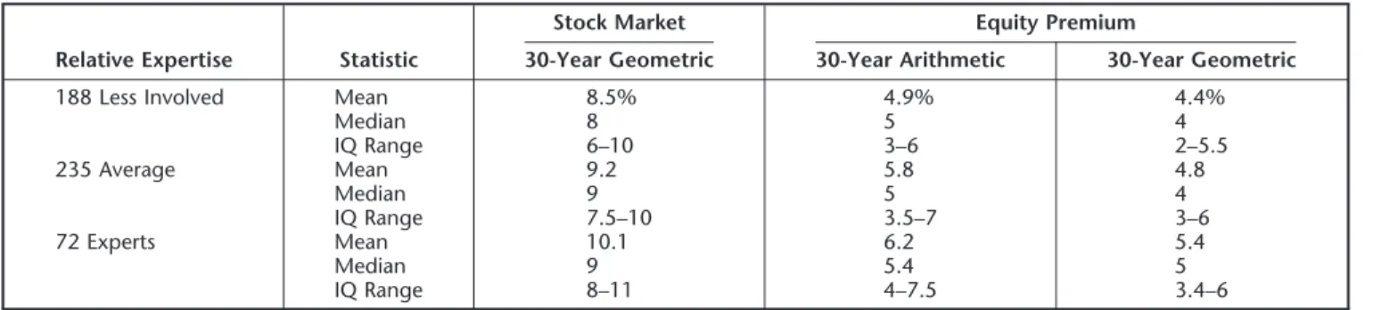
In his most current survey, Welch (2001) com-piled the responses of about 500 financial econo-mists to determine their consensus ERP. He found the average arithmetic estimate for the 30-year ERP, relative to Treasury bills, to be 5.5% and the one-year arithmetic ERP consensus to be 3.4%. Welch deduced from the average 30-year geometric equity return estimate of 9.1% that the

22_{A “hurdle” rate is a benchmark cost of capital used to evaluate}

projects to accept (expected returns greater than hurdle rate) or reject (expected returns less than hurdle rate). Graham and Harvey (2002) claim three-fourths of the CFOs use CAPM to estimate hurdle rates.

arithmetic equity return forecast was approxi-mately 10%.23

Welch’s survey question allowed participants to self-select into different categories based on their knowledge of ERP. The results indicate that the responses of the less ERP-knowledgeable partici-pants were more pessimistic than those of the self-reported experts. The experts gave 30-year estimates that are 30 –150 basis points above the estimates of the nonexpert group.

Table 8 shows that there may be a “lemming” effect, especially among economists who are not directly involved in the ERP question. Stated differ-ently, all the academic and popular press—together with the prior 1998 Welch survey (which had an ERP consensus of about 7%)— could have condi-tioned the nonexpert, or the “less involved,” that the expected ERP was lower than historic levels.

14. T

B

A

Benartzi and Thaler (1995) analyzed the ERP puzzle from the viewpoint of prospect theory (Kahneman and Tversky 1979). Prospect theory allows asymmetric “loss aversion”—the fact that individuals are more sensitive to potential loss than gain—as one of its central tenets (see Tver-sky and Kahneman 1991 and Barberis et al. 2001 for a current survey of the applications of pros-pect theory to finance). Once an asymmetry in risk aversion is introduced into the model of the

rational representative investor or agent, the un-usual risk aversion problem raised initially by Mehra and Prescott (1985) can be “explained” by parameters within this behavioral model of deci-sion making under uncertainty.

Stated differently, given the historical ERP se-ries, there exists a model of investor behavior that can produce those or similar results. Benartzi and Thaler (1995) combined loss aversion with “men-tal accounting”—the behavioral process people use to evaluate their status relative to gains and losses compared to expectations, utility, and wealth—to get “myopic loss aversion.” In partic-ular, mental accounting for a portfolio needs to take place infrequently in order to reduce the chances of observing loss versus gain. The au-thors concede that there is a puzzle with the standard expected utility-maximizing paradigm but that the myopic loss aversion view may re-solve the puzzle. The authors’ views are not free of controversy; any progress applying behavioral concepts to the ERP puzzle is sure to match the advance of behavioral economics as a whole.

The adoption of other behavioral aspects of investing also may provide support for the histor-ical patterns of ERPs we see from 1802–2002. For example, as the true nature of risk and rewards has been uncovered by the virtual army of 20th

century researchers, and as institutional inves-tors held sway in the latter 50 years of the cen-tury, the demand for higher rewards seen in the later historical data may be a natural and rational response to the new and expanded information set. Dimson et al. (2002, figs. 4 – 6) displays in-creasing real U.S. equity returns of 6.7%, 7.4%, 8.2% and 10.2% for periods of 101, 75, 50 and 25

23

For the Ibbotson 1926 –2002 data, the arithmetic return is about 190 basis points higher than the geometric return, rather than the inferred 90 basis points. This suggests the participants’ beliefs, in Welch’s study, may not be internally consistent.

Table 8

Differences in Forecasts across Expertise Level

Relative Expertise Statistic

Stock Market Equity Premium

30-Year Geometric 30-Year Arithmetic 30-Year Geometric

188 Less Involved Mean 8.5% 4.9% 4.4%

Median 8 5 4 IQ Range 6–10 3–6 2–5.5 235 Average Mean 9.2 5.8 4.8 Median 9 5 4 IQ Range 7.5–10 3.5–7 3–6 72 Experts Mean 10.1 6.2 5.4 Median 9 5.4 5 IQ Range 8–11 4–7.5 3.4–6

years, ending in 2001, consistent with this “risk-learning” view.

15. T

N

10 Y

The “next 10 years” is an issue that Campbell and Diamond discuss when reviewing Social Securi-ty’s assumptions and Campbell and Shiller (2001) address, either explicitly or implicitly. Experts evaluating Social Security’s proposals predicted that returns during the “next 10 years,” indicat-ing a period beginnindicat-ing around 2000, were likely to be below the historical return. However, a histor-ical return was recommended as appropriate for the remaining 65 of the 75 years to be projected. The period Campbell and Shiller discussed is ap-proximately 2000 –2010. Based on the then-cur-rent state of valuation ratios, they predicted lower stock market returns over “the next 10 years.”

These expert predictions, and other pessimistic low estimates, have already come to fruition as market results from 2000 through 2002.24 The U.S. equities market has decreased 37.6% since 1999, or an annual decrease of 14.6%. Although these forecasts have proved to be accurate in the short term, for future long-run projections, the market is not at the same valuation today as it was when these conditional estimates were orig-inally given. Therefore, actuaries should be wary of using the low long-run estimates made prior to the large market correction of 2000 –2002.

16. T

I

P

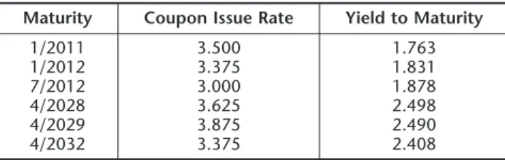
S

Several of the ERP researchers referred to TIPS when considering the real risk-free rates. Histor-ically, they adjusted Treasury yields downward to a real rate by an estimate of inflation, presumably for the term of the Treasury security. The modern era data in Table 3 show a low real long-term, risk-free rate of return (2.2%). This contrasts with the initial TIPS issue yields of 3.375%.25 Some researchers use those TIPS yields as (market) forecasts of real risk-free returns for intermediate and long-horizon, together with reduced (real)

equity returns, to produce low estimates of ex anteERPs. None consider the volatility of TIPS as indicative of the accuracy of their ERP estimate. Table 9 shows a 2003 market valuation of 10-and 30-year TIPS issued in 1998 –2002. Note the large 90 –180 basis point decrease in the current “real” yields from the issue yields even just a year later for some issues. While there can be several explanations for the change (revaluation of the inflation option, flight to Treasury quality, pau-city of 30-year Treasuries), the use of these cur-rent “real” risk-free yields, with fixed expected returns, would raise ERPs by at least 1%.

17. C

This paper has sought to bring the essence of recent research on the ERP to practicing actuar-ies. The researchers covered here face the same ubiquitous problems that actuaries face daily: Do I rely on past data to forecast the future (costs, premiums, investments), or do I analyze the past and apply informed judgment as to future differ-ences, if any, to arrive at actuarially fair fore-casts? Most of the ERP estimates lower than the unconditional historical estimate have an undue reliance on recent lower dividend yields (without a recognition of capital gains26_{) and/or on data}

prior to 1926.

Despite a spate of research suggesting ex ante ERPs lower than recent realized ERPs, actuaries should be aware of the range of estimates covered here (Appendix B); be aware of the underlying

24

The Social Security Advisory Board (2002) will revisit the 75-year rate of return assumption during 2003.

25

TIPS were introduced by the Treasury in 1996 with the first issue in January 1997.

26

Under the current U.S. tax code, capital gains are tax-advantaged relative to dividend income for the vast majority of equityholders (households and mutual funds are 55% of the total equityholders, according to the Federal Flow of Funds, 2002 Q3, Table L-213). Curiously, the reverse is true for property-liability insurers because of the 70% stock dividend exclusion afforded insurers.

Table 9

Inflation-Indexed Treasury Securities

Maturity Coupon Issue Rate Yield to Maturity

1/2011 3.500 1.763 1/2012 3.375 1.831 7/2012 3.000 1.878 4/2028 3.625 2.498 4/2029 3.875 2.490 4/2032 3.375 2.408

assumptions, data, and terminology; and be aware that their independent analysis is required before adopting an estimate other than the his-torical average. We believe that the Ibbotson and Chen (2003) layout, reproduced here as Appen-dix D, offers the actuary both an understanding of the fundamental components of the historical ERP and the opportunity to change the estimates based on good judgment and supportable beliefs. We believe that reliance solely on “expert” survey averages, whether of financial analysts, academic economists, or CFOs, is fraught with risks of sta-tistical bias in estimates of theex ante ERP.

It is dangerous for actuaries to engage in sim-plistic analyses of historical ERPs to generate ex ante forecasts that differ from the realized mean.27The research we have catalogued in Ap-pendix B, the common level ERPs estimated in Appendix C, and the building-block (historical) approach of Ibbotson and Chen (2003) in Appen-dix D all discuss important concepts related to both ex post and ex ante ERPs and cannot be ignored in reaching an informed estimate.

For example, Wendt (2002) concluded that a lin-ear relationship with interest rates is a better pre-dictor of future returns than is a “constant” ERP based on the average historical return. He arrived at this conclusion by estimating a regression equation relating long bond yields with 15-year geometric mean market returns starting monthly in 1960.28

Wendt’s findings are misleading. First, there was no significant relationship between short-, intermedi-ate-, or long-term income returns over 1926 –2002 (or 1960 –2002) and annual ERPs, as evidenced by simple regressions using Ibbotson data.29Second, if the linear structural equation indeed held, there would be no need for an ERP since the (15-year) return could be predicted within small error bars. Third, there is always a negative bias introduced when geometric averages are used as dependent variables (Brennan and Schwartz 1985). Finally,

the results are likely to be spurious due to the high autocorrelations of the target and independent variables; an autocorrelation correction would eliminate any significant relationship of long yields to the ERP.

Actuaries also should be aware of the variability of both the ERP and risk-free rate estimates dis-cussed in this paper (see Tables 4 and 9). All too often, return estimates are made without noting the error bars, and that can lead to unexpected “surprises.” As one example, recent research by Longstaff (2004) proposes that a 1991–2001 “flight to quality” has created a valuation pre-mium (and lowered yields) in the entire yield curve of Treasuries. He finds a 10 –16 basis point liquidity premium throughout the zero coupon Treasury yield curve. He translates that into a 10 –15% pricing difference at the long end. This would imply a simple CAPM market estimate for the long horizon might be biased low.

Finally, actuaries should know that the re-search catalogued in Appendix B is not definitive. No simple model of ERP estimation has been uni-versally accepted. Undoubtedly, there will be still more empirical and theoretical research into this data-rich financial topic. We await the potential advances in understanding the return process that the behavioral view may uncover.

18. P

S

: A

A–D

We provide four appendices that catalogue the ERP approaches and estimates discussed in the paper. Actuaries, in particular, should find the numerical values, and descriptions of assump-tions underlying those values helpful for valuation work that adjusts for risk. Appendix A provides the annual data from 1926 through 2002 from Ibbotson Associates referred to throughout this paper. The equity risk premium shown is a simple difference of the arithmetic stock returns and the arithmetic U.S. Treasury bill total returns.

Appendix B is a compilation of articles and books related to the ERP. The puzzle research section contains the articles and books that were most re-lated to addressing the ERP puzzle.30 Appendix B

27_{ERPs are derived from historical or expected after-corporate-tax}

returns. Pre-tax returns depend uniquely on the tax schedule for the differing sources of income.

28

Fifteen-year mean returns ⫽ 2.032 (Long Government Yield) – 0.0242, R2_⫽0.882.

29

Thep-values on the yield variables in an annual ERP/yield regres-sion using 1926 –2002 annual data are 0.1324, 0.2246, and 0.3604 for short-, intermediate-, and long-term yields, respectively, with adjusted R-square values virtually zero.

30

Additional references are included, in the table, that were not previously discussed (see Cornell 1999, Dimson et al. 2002, Siegel 1999, Siegel 2002, and Grinold and Kroner 2002 (Barclays Global Investors).

gives each source, along with risk-free rate and ERP estimates and further details collected from each source. For example, we show the data period used, if applicable, and the projection period. We also list the general methodology used in the reference. Footnotes give additional details on the sources’ intent.

Appendix C adjusts all the ERP estimates to a short-horizon, arithmetic, unconditional ERP es-timate. We begin with the authors’ estimates for a stock return (the risk-free rate plus the ERP esti-mate). Next, we make adjustments if the ERP “type” given by the author(s) is not provided in this format. For example, to adjust from a geo-metric to an arithmetic ERP estimate, we adjust upward by the 1926 –2002 historical difference in the arithmetic large-company stocks’ total return and the geometric large-company stocks’ total return of 2%. Next, if the estimate is given in real instead of nominal terms, we adjust the stock return estimate upward by 3.1%, the 1926 –2002 historical return for inflation.

We make an approximate adjustment to move the estimate from a conditional to unconditional estimate based on Fama and French (2002) where they make similar adjustments for the bi-ases in a dividend or earnings growth model. For the 1951–2000 period, Fama and French use an adjustment of 1.28% for the dividend growth model and 0.46% for the earnings growth model (Table 4, p. 655). Using their adjustment method and the data provided in Fama and French’s table 1, the 1872–2000 period would require a 0.82%

adjustment and the 1872–1950 period would re-quire a 0.54% adjustment using a dividend growth model. Therefore, we selected the lowest adjust-ment (0.46%) from the different time periods and models as a minimum adjustment from a condi-tional estimate to an uncondicondi-tional estimate of market returns. Finally, we subtract the 1926 – 2002 historical U.S. Treasury bills’ total return to arrive at an adjusted ERP.

These adjustments are only approximations be-cause the various sources rely on different under-lying data, but the changes in the ERP estimate should reflect the underlying concept that differ-ent “types” of ERPs cannot be directly compared and require some attempt to normalize the vari-ous estimates.

Appendix D reproduces a table from Ibbotson and Chen (2003) that breaks down historical re-turns using various methods discussed in their paper, including forward-looking estimates. Sum-marized formulas from Ibbotson and Chen’s pa-per are also displayed.

A

The authors acknowledge the helpful comments from participants in the 2003 Bowles Symposium, Louise Francis of Francis Analytics & Actuarial Data Mining Inc., and four anonymous referees. The authors would also like to thank Jack Wilson for supplying his data series from Wilson and Jones (2002).

Appendix A

Ibbotson Market Data 1926 –2002

Year Common stocks U.S. Treasury Bills Arithmetic Short-Horizon Year Common stocks U.S. Treasury Bills Arithmetic Short-Horizon Total Annual Returns Total Annual Returns Equity Risk Premia Total Annual Returns Total Annual Returns Equity Risk Premia 1926 11.62% 3.27% 8.35% 1927 37.49 3.12 34.37 1928 43.61 3.56 40.05 1929 ⫺8.42 4.75 ⫺13.17 1930 ⫺24.90 2.41 ⫺27.31 1931 ⫺43.34 1.07 ⫺44.41 1932 ⫺8.19 0.96 ⫺9.15 1933 53.99 0.30 53.69 1934 ⫺1.44 0.16 ⫺1.60 1935 47.67 0.17 47.50 1936 33.92 0.18 33.74 1937 ⫺35.03 0.31 ⫺35.34 1938 31.12 ⫺0.02 31.14 1939 ⫺0.41 0.02 ⫺0.43 1940 ⫺9.78 0.00 ⫺9.78 1941 ⫺11.59 0.06 ⫺11.65 1942 20.34 0.27 20.07 1943 25.90 0.35 25.55 1944 19.75 0.33 19.42 1945 36.44 0.33 36.11 1946 ⫺8.07 0.35 ⫺8.42 1947 5.71 0.50 5.21 1948 5.50 0.81 4.69 1949 18.79 1.10 17.69 1950 31.71 1.20 30.51 1951 24.02 1.49 22.53 1952 18.37 1.66 16.71 1953 ⫺0.99 1.82 ⫺2.81 1954 52.62 0.86 51.76 1955 31.56 1.57 29.99 1956 6.56 2.46 4.10 1957 ⫺10.78 3.14 ⫺13.92 1958 43.36 1.54 41.82 1959 11.96 2.95 9.01 1960 0.47 2.66 ⫺2.19 1961 26.89 2.13 24.76 1962 ⫺8.73 2.73 ⫺11.46 1963 22.80 3.12 19.68 1964 16.48 3.54 12.94 1965 12.45 3.93 8.52

Source:Authors’ calculations using Ibbotson Associates (2003a, pp. 38 –39).

1966 ⫺10.06% 4.76% ⫺14.82% 1967 23.98 4.21 19.77 1968 11.06 5.21 5.85 1969 ⫺8.50 6.58 ⫺15.08 1970 4.01 6.52 ⫺2.51 1971 14.31 4.39 9.92 1972 18.98 3.84 15.14 1973 ⫺14.66 6.93 ⫺21.59 1974 ⫺26.47 8.00 ⫺34.47 1975 37.20 5.80 31.40 1976 23.84 5.08 18.76 1977 ⫺7.18 5.12 ⫺12.30 1978 6.56 7.18 ⫺0.62 1979 18.44 10.38 8.06 1980 32.42 11.24 21.18 1981 ⫺4.91 14.71 ⫺19.62 1982 21.41 10.54 10.87 1983 22.51 8.80 13.71 1984 6.27 9.85 ⫺3.58 1985 32.16 7.72 24.44 1986 18.47 6.16 12.31 1987 5.23 5.47 ⫺0.24 1988 16.81 6.35 10.46 1989 31.49 8.37 23.12 1990 ⫺3.17 7.81 ⫺10.98 1991 30.55 5.60 24.95 1992 7.67 3.51 4.16 1993 9.99 2.90 7.09 1994 1.31 3.90 ⫺2.59 1995 37.43 5.60 31.83 1996 23.07 5.21 17.86 1997 33.36 5.26 28.10 1998 28.58 4.86 23.72 1999 21.04 4.68 16.36 2000 ⫺9.11 5.89 ⫺15.00 2001 ⫺11.88 3.83 ⫺15.71 2002 ⫺22.10 1.65 ⫺23.75 Mean 12.20 3.83 8.37 Std dev 20.49 3.15 20.78