Probabilistic Methods for Finding People
S. IOFFE AND D.A. FORSYTH
Computer Science Division, University of California at Berkeley, Berkeley, CA 94720 [email protected]
Received July 2, 2000; Revised March 12, 2001; Accepted March 12, 2001
Abstract. Finding people in pictures presents a particularly difficult object recognition problem. We show how to find people by finding candidate body segments, and then constructing assemblies of segments that are consistent with the constraints on the appearance of a person that result from kinematic properties. Since a reasonable model of a person requires at least nine segments, it is not possible to inspect every group, due to the huge combinatorial complexity.
We propose two approaches to this problem. In one, the search can be pruned by using projected versions of a classifier that accepts groups corresponding to people. We describe an efficient projection algorithm for one popular classifier, and demonstrate that our approach can be used to determine whether images of real scenes contain people. The second approach employs a probabilistic framework, so that we can draw samples of assemblies, with probabilities proportional to their likelihood, which allows to draw human-like assemblies more often than the non-person ones. The main performance problem is in segmentation of images, but the overall results of both approaches on real images of people are encouraging.
Keywords: object recognition, human detection, probabilistic inference, grouping correspondence search
1. Introduction
Finding people in images is a difficult task, due to the high variability in the appearance of people. This vari-ability may be due to the configuration of a person (e.g., standing vs. sitting vs. jogging), the pose (e.g. frontal vs. lateral view), clothing, and variations in illumination. There are two usual strategies for object recognition:
• Search over model parameters (kinematic variables, camera parameters, etc.) using a comparison be-tween a predicted view of the object and the im-age. This problem is often stated as optimization of an objective function, which measures the similarity between the predicted and the actual views. This is usually called thetop-downapproach.
• Assemble image features into increasingly large groups, using the current group as a rough hypothesis
about the object identity to select the next grouping activity. This is usually called the bottom-up
approach.
1.1. Why Proceed Bottom-Up?
Current activities in vision emphasize top-down recog-nition and tracking. There are three standard ap-proaches to finding people described in the literature. Firstly, the problem can be attacked by template match-ing (e.g. (Oren et al., 1997), where upright pedes-trians with arms hanging at their side are detected by a template matcher; (Niyogi and Adelson, 1995; Liu and Picard, 1996; Cutler and Davis, 2000), where walking is detected by the simple periodic structure that it generates in a motion sequence; (Haritaoglu et al., 2000; Wren et al., 1997), which rely on back-ground subtraction—that is, a template that describes
“non-people”). Matching templates to people (rather than to the background) is inappropriate if people are going to appear in multiple configurations, because the number of templates required is too high.
This motivates the second approach, which is to find people by finding faces (e.g. (Poggio and Sung, 1995; Rowley et al., 1996a, 1996b; Rowley et al., 1998a, 1998b; Sung and Poggio, 1998)). The approach is most successful when frontal faces are visible.
The third approach is to use the classical technique of search over correspondence (this is an important early formulation of object recognition; the techniques we describe have roots in (Faugeras and Hebert, 1986; Grimson and Lozano-P´erez, 1987; Thompson and Mundy, 1987; Huttenlocher and Ullman, 1987)). In this approach, we search over correspondence between image configurations and object features. There are a variety of examples in the literature (for a variety of types of object; see, for example, (Huang et al., 1997; Ullman, 1996)). Perona and collaborators find faces by searching for correspondences between eyes, nose and mouth and image data, using a search controlled by probabilistic considerations (Leung et al., 1995; Burl et al., 1995). Unclad people are found by (Forsyth et al., 1996; Forsyth and Fleck, 1999), using a correspon-dence search between image segments and body seg-ments, tested against human kinematic constraints.
It is difficult to evaluate the correspondences between image regions and model parts and reliably choose the best ones. A crucial difficulty in both finding and tracking people is that extended, straight, coherent image regions—which could be body segments—can be relatively common. This means in turn that any objective function is going to have a local extremum where a hypothesized body segment lies over that re-gion. The result is a tendency for trackers to drift or finding methods to become confused. The problem is simplified for the trackers since the configuration in a frame can be used to start the search for the next frame, but local extrema still present a significant problem and cause body parts to be lost due to occlusions, to other objects nearby that look like body parts, or to espe-cially rapid motions. In addition, most trackers need to be started by hand, by specifying the configuration in the initial frame.
It is natural to try and simplify matters with a contin-uation method: take a series of simplified versions of the evaluation function, search the simplest, and use the result as a start point for a search on a less simple ver-sion, ending at an extremum of the original evaluation
function. The annealed particle filter of (Deutscher et al., 2000) uses this strategy, but apparently cannot deal with much clutter because it creates too many dif-ficult peaks. Furthermore, using this strategy to find and track people requires a detailed search of a high di-mensional domain (the number of people being tracked times the number of parameters in the person model plus camera parameters). This implies that a method is needed that is able to explore large search spaces and thus provide an efficient alternative to blank search.
Bottom-up methods offer the promise of signifi-cantly reduced search, but have become unpopular because it appears to be very difficult to realize this promise. A typical bottom-up method would (1) detect a variety of features and then (2) group these features incrementally into assemblies, using a grouping pro-cedure that takes into account the features in a group before adding features. An example of this process— which dates back at least to (Binford, 1971)—would in-volve finding objects by: (1) finding edges; (2a) pairing edge fragments that appear to lie locally on a general-ized cylinder; (2b) collecting pairs that together appear to lie on a generalized cylinder; (2c) collecting pairs of straight homogeneous generalized cylinders with roughly constant cross-section which lie nearby and (2d) asserting that all such pairs could be arms. There are many instances of this line of reasoningwhich does not require the use of any particular primitive(finding curved objects in range data (Agin, 1972; Nevatia and Binford, 1977); finding people in images (Forsyth et al., 1996); finding lamps and mugs in images (Dickinson et al., 1992; Ulupinar and Nevatia, 1988; Zerroug and Nevatia, 1999) amongst others). Note that the group-ing process is maintaingroup-ing an increasgroup-ingly more pre-cise hypothesis of the object’s identity, which is used to direct grouping activities. The success of the method depends on being able to supply a series of grouping activities that: (1) can cope with bad features; (2) have little ambiguity at each stage about what should be done—because this results in search; and (3) can ro-bustly recognize many different types of object.
Many researchers have modeled a person as a kine-matic chain, and recognized people as collections of generalized cylinders, subject to constraints given by the kinematics of human joints. This approach has been successful in tracking (e.g., (Gavrila and Davis, 1996; O’Rourke and Badler, 1980)). Generally, the tracker is initialized by marking the subject’s configuration in the first frame, and the configuration is updated from frame to frame. In (Hogg, 1983) and (Rohr, 1993), the
frame-to-frame configuration update is accomplished by a search of the parameter space to minimize a model-to-image matching cost. Often, the update involves non-linear optimization (e.g., using gradient descent) to find the new configuration, where the old one is used to start the search (Bregler and malik, 1998; Rehg and Kanade, 1994).
The dichotomy between the top-down and bottom-up approaches is not precise. For example, in the peo-ple finding method of (Felzenszwalb and Huttenlocher, 2000), theglobal extremumof the objective function is found by first computing a response to the body-part filter at each orientation, position and scale (using con-volution with a bank of filters), and then extracting the optimal group of body parts using dynamic program-ming. To be able to find the global extremum, however, they restrict the class of object models: the appearance model for the body parts is constrained to have a par-ticular size and color, so that convolution could be used for body-part detection; the kinematic model must have the form of a tree so that the optimal configuration can be found efficiently. Furthermore, their framework lacks a discriminative component, and the system can-not determine whether a given image contains a person, but can only guess the person’s configuration if one is known to be present.
In our work, we avoid such constraints and still are able to efficiently find people by pruning the search— that is, ignoring entire regions of the search space which have been determined not to contain the solution.
1.2. Outline
We assume that an image of a human can be decom-posed into a set of distinctive segments, so that there is a segment of each type in each image (so that in each image a correspondence from model segments to image segments can be established). While this repre-sentation is restrictive, since body parts may often be absent due to either occlusion or their unusual appear-ance, we show that it can be used to detect and count people.
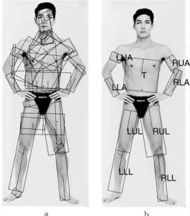
A simple segment detector is used to find image re-gions that could correspond to body parts. However, the appearance of limbs is not nearly as distinctive as that of the whole body (especially in the absence of cues such as the skin color), and thus many spurious body parts are found along with the actual ones (Fig. 1(a)). In addition, the correspondence between image regions and the body parts is hard to establish since many body
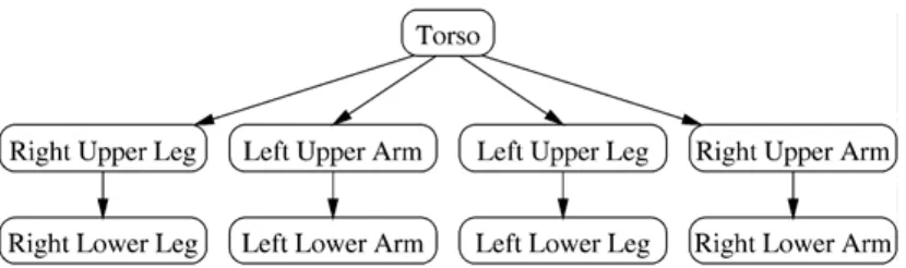
Figure 1. (a) All segments extracted for an image. (b) A labeled segment configuration corresponding to a person, whereT=torso, LUA=left upper arm, etc. The head is not marked because we are not looking for it with our method.
parts are indistinguishable from one another (e.g., the two upper arms). However, the human body is subject to rather strong kinematic constraints. For example, if two segments have been matched to a left upper arm and a left lower arm, then the lengths of these seg-ments and their relative positions are constrained so as to correspond to a possible elbow configuration.
The goal of this paper is to demonstrate that we can efficiently group the candidate segments found in an image (image segments) intoassemblies —human-looking groups of image segments, with each element marked with a label specifying to which body part that segment corresponds (see Fig. 1(b)). Alternatively, we can think of a matching of the model to the image, whereby each model segment is coupled with an im-age segment.
The main issue with grouping is that the brute force approach of testing each combination of segments doesn’t work because of the huge number of such as-semblies (e.g., for 100 segments in the image, we have about 1018assemblies with 9 segments (torso plus two segments per limb)). However, we can make the search much more manageable if we use the fact that, for most segment groups, it is impossible to add other segments found in the image in such a way that the resulting as-sembly looks like a person. For example, if it has been detected that two segments cannot represent the upper
and lower left arm, as in Fig. 6(a), then no assembly containing them will correspond to a person, and would not need to be considered.
We will show:
• How to represent body parts (Section 2) and learn models of relationships between them (Sections 3.3.2 and 4.3.2).
• How to prune the search. In Sections 3.3.3 and 4.3.4, we will demonstrate how we can, for a partial model-to-image matching (an assembly with some ments missing), determine that, no matter what seg-ments are added to an assembly, it could not look like a person. In that case the current branch of the interpretation tree could be ignored.
• How to structure the search to make it efficient. In Sections 3.3.4 and 4.3.3, we give strategies for in-crementally adding image segments to an assembly so that the pruning mechanism could be effectively exploited.
• That these methods can find and count people in im-ages (Section 5).
1.3. Representation
As in much of the previous work mentioned above, we model the person as a collection of cylinders, and an im-age of a person as a collection of bar-shapedsegments. We ignore a person’s head. Bars can be detected us-ing image edges, segmentation techniques such as nor-malized cuts (Shi and Malik, 1997), or motion cues if the image is a part of a video sequence. We picked the simplest type of segment detector, which looks for pairs of parallel edges. Such a detector is described in Section 2 and will, much of the time, detect all the body parts of a person, but will also produce many spurious segments for non-person image regions. This is accept-able, since kinematic constraints will help discriminate human segments from spurious ones.
By adopting the simplest segment-detection mech-anism, we are able to concentrate on the search pro-cess. Even though our segment detector can deal with only one type of body part (bars, and not, for example, the head) and produces many spurious segments, kine-matic constraints are a powerful cue as to which seg-ments are the actual body parts, and we show that our search and pruning strategies use these constraints ef-fectively. However, many of the failures of our method are due to missing or inaccurately detected segments, which suggests that our inference method is effective, but the overall system would benefit from an improved
segment-finder. We discuss such improvements in Section 6.
The disadvantage of using our segment detector is that the range of images we can use is limited: our sub-jects may not wear baggy clothes. In this paper, we restrict ourselves to images of models wearing swim-suits or no clothes. However, the grouping process is independent of how the body segments are repre-sented. Therefore, the restrictions imposed by the way we model the segments can be overcome. Section 6 dis-cusses detecting more than one type of segments (e.g., limbs and the face), and handling clothes.
In this paper, we show two ways of efficiently as-sembling potential body parts into human assemblies. These two methods use different models of a person, which leads to different search and pruning strategies.
Classification: In Section 3 we show how to effi-ciently learn atop-level classifierthat discriminates human assemblies of segments from non-human ones, and how to efficiently extract all assemblies in the image that look like people by adding segments to assembliesincrementally. The efficiency is achieved by pruning small assemblies, usingprojected classi-fiers. We describe how to derive projected classifiers from the top-level one. The pruning of subtrees of the interpretation tree is model-driven, which means that we backtrack the search if an assembly has been found such that, no matter what segments are added to it, the result will not look like a person.
Inference: In Section 4, we demonstrate a proba-bilistic method that uses asoft classifier, which asso-ciates a measure of likelihood of a person with each assembly, rather than a binary “person/non-person” decision. We describe a method for detecting people by sampling from the likelihood, and this method is made efficient by sampling sub-assemblies of in-creasing size, usingimportance sampling. The prun-ing is accomplished by first computprun-ing upper bounds on the likelihoods of sub-assemblies (using dynamic programming), and using these bounds to define the intermediate distributions, from which the sub-assemblies are sampled. Such pruning is data-driven: an assembly is no longer considered if the computed bounds indicate that noimage segmentscan be added to make a human assembly.
2. Finding Segments
It is usual to model the appearance of body parts in the image as bars (i.e., projections of straight cylinders),
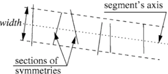
Figure 2. A symmetry: the two edgels (dashed lines) are symmet-rical about the symmetry axis (dotted). We represent symmetries by their sections (solid line), which are line segments that connect the midpoints of the two edgels.
e.g. (Bregler and Malik, 1998; Gavrila and Davis, 1996; Hogg, 1983; O’Rourke Badler, 1980; Rohr, 1993). This seems to be a reasonable and natural representation, which, as we show in this paper, delivers promising results. We use pictures of people wearing swimsuits or no clothes, which allows us to detect bars by grouping parallel edges. We discuss the problem of body-part detection for clothed people in Section 6.
To find rectangular approximations to candidate body segments, we extract edges and identify sets of edge elements that form, approximately, pairs of paral-lel line segments (which become the length-wise sides of the rectangular segments). This grouping process is hierarchical, whereby we first identify “symmetries”— pairs of symmetrical edgels—and then group them (Brady and Asada, 1984; Brooks, 1981).
Two edges constitute a symmetry if, within some margin of error, they are reflections of each other about some symmetry axis. The verification is done by con-sidering thesection—the line connecting the midpoints of the two edgels—and finding the axis perpendicular to the section and passing through its midpoint. We then declare the edgel pair a symmetry if the angles the edgels form with the axis are sufficiently similar and small (Fig. 2).
Each edgel can be a part of zero, one or more sym-metries. We will now group symmetries into segments. A set of symmetries constitutes a segment if the lengths of their sections are roughly the same (this corresponds to the segment’swidth), the midpoints of their sections are roughly on the same line (the segment’s axis), to which the sections are perpendicular. There should also not be large gaps between symmetries of the same seg-ment (Fig. 3).
We group symmetries by fixing the number of seg-ments and searching for the best segment parameters (their axes and widths) and assignments of symme-tries to segments (each symmetry being assigned to one of the segments or to noise). This can be formu-lated as an optimization problem (segment parameters)
Figure 3. The segment finder groups symmetries into segments. The EM algorithm finds the optimal positions of the segments’ axes and the widths, and also estimates the posterior probabilities that a given symmetry is assigned to a particular segment or to noise.
in the presence of missing data (labels representing segment assignment for each symmetry). The natural method for solving such a problem is the Expectation-Maximization algorithm (Dempster et al., 1977). This algorithm produces the optimal segment parameters and posterior probabilities for the assignment labels.
Each segment is represented with asymmetry axis
and awidth. Each symmetry has a label showing which segment (or noise) it belongs to. A symmetry fits a seg-ment best when the midpoint of the symmetry lies on the segment’s symmetry axis, the endpoints lie half a segment width away from the axis, and the symme-try is perpendicular to the axis. This yields the condi-tional likelihood for a symmetry given a segment as a four-dimensional Gaussian (two numbers for each endpoint), and an EM algorithm can now fit a fixed number of segments to the symmetries. After that, we determine where each segment begins and ends by find-ing the range of symmetries for which this segment has the largest posterior. If there is a large gap between these symmetries (that is, symmetries from different image regions are attributed to the same segment), then the segment is broken into two or more pieces. The Fig. 4 shows example images produced by the segment finder. Note that the segments we have found do not have an orientation (for instance, if we hypothesize that one of them is the torso, we don’t know which end corre-sponds to the shoulders and which to the hips). Another problem is that if a limb is straight in an image, then only a single segment is obtained rather than the upper and lower halves. We deal with this by replacing each segment with its two oriented versions, and also split-ting each segment in half length-wise and adding both halves to the segment set (Fig. 5). We also add a con-straint, when grouping segments, that if one of the seg-ment halves was labeled as a lower limb, then the other half of the same segment has to be the corresponding upper limb.
Figure 4. An example run of the segment finder. (top) A set of symmetries obtained for an image. Each symmetry is represented by its section. We show every 4th symmetry to avoid clutter. (bottom) The EM algorithm fits a fixed number of rectangular segments to the symmetries. These are the candidate body segments which become the input to our assembly-builder (grouper).
Figure 5. Each segment found using EM is replaced with its two oriented versions, each of which is then split in half. This procedure allows us to deal with the situation when a single segment is found for a straight limb. Also, it allows us to specify, for example, which end of a lower-arm segment is the wrist and which is the elbow. The arrows within the segments indicate their orientation.
It is not necessary to get the segments exactly right, as the kinematic information used in grouping them is powerful enough to handle inaccuracies.
3. Finding People Using Classification
After the segment detector has identified the image re-gions that could, possibly, correspond to human body parts, we need to assemble theseimage segmentsinto groups that look like people. The brute-force approach of classifying every segment group doesn’t work be-cause of the huge number of such assemblies. Instead, we build such assemblies incrementally, by sequen-tially considering groups of increasing size, and grow-ing a group by trygrow-ing to add another image segment to it. The advantage of incremental search is that it could be made quite efficient if we can detect early that a group of segments couldnotbe a part of a person, no matter what other segments are added. For example, if two segments can under no circumstances represent the upper and lower left arm, as in Fig. 6(a), then no as-sembly containing them will correspond to a person.
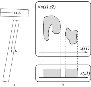
Figure 6. (a) Two segments that cannot correspond to the left up-per and lower arm. Any configuration where they do can be re-jected using a prore-jected classifier regardless of the other segments that might appear in the configuration. (b) Projecting a classifier C{(l1,s1), (l2,s2}. We are considering two features, one of them,
x(s1), depending only on the segment labeled asl1, and the other,
y(s1,s2), depending on both segments. (top) The shaded area is the
volume classified as positive, for the feature set{x(s1),y(s1,s2)}.
(bottom) Finding the projectionCl1amounts to projecting off the
This means that we can prune all model-to-image correspondences containing this one. This observation dates back to (Grimson and Lozano-P´erez, 1987), who use it to prune an interpretation tree of correspon-dences. We show how to derive this pruning mechanism in a principled way from a single, learned classifier.
We learn thetop-level classifieras the classifier that takes an assembly of 9 segments labeled as the 9 differ-ent body parts, and determines whether the assembly corresponds to a person. From that classifier we con-struct a family of tests that determine, for a group of 8 or fewer segment-label pairs, whether it may be possi-ble for this group to be augmented to a full 9-segment assembly that is classified as a person by the top-level classifier. If it has been determined that no such aug-mentation is possible for an assembly, then it, and all the assemblies containing it, can be rejected. Each test used for the early rejection is obtained from the top-level classifier byprojection. By projecting a classifier, we mean obtaining a new classifier that uses a subset of features used by the original one, so that the volume classified as “positive” by the projected classifier is the projection of the positive volume of the original classi-fier onto a subspace of the feature space. An example of a projected classifier is given in Fig. 6(b).
Projected classifiers allow us to search for human semblies efficiently, by incrementally considering as-semblies of increasing size. At each stage, an assembly is discarded if it is classified as “non-human” by the cor-responding project classifier—that is, if no segments can be added to the assembly to obtain a 9-segment human assembly. We grow the assemblies that are not discarded by trying to pair them with each remaining image segment. The search becomes efficient if many assemblies are discarded at an early stage, so that, for a subset of labels, only a small fraction of the set of all the assemblies corresponding to that subset need to be considered.
By introducing projected classifiers we do not make our system more prone to overfitting, since each pro-jected classifier is not learned independently, but rather isdeterministically derived from the top-level classi-fier. It follows from the definition of the projected clas-sifier that using them to discard smaller segment groups does not affect the final result: the set of human assem-blies found in the image does not change. The gain from the use of projected classifiers is only in efficiency: they allow us to find every human assembly in the image without considering all the possible 9-segment groups.
In this section, we describe how to learn aclassifier
that identifies human assemblies, how to organize the search so that assemblies are builtincrementally, and how toprojectthe classifier so that theprojected clas-sifierscould be used to determine that a segment group could not be a part of a human assembly and thus prune the search.
3.1. Building Segment Configurations
Suppose that the set of candidate segments has been found for an image. We will define anassemblyas a set
A= {(l1,s1), (l2,s2), . . . , (lk,sk)}
of pairs where each segmentsiis labeled with thelabel
li. The segments{si}are a subset of candidate image segments, and each labellispecifies what body part is matched to the the segmentsiand can thus take on one of the 9 distinct values (li ∈ {
T
,LUA
,RLL
, . . .}), cor-responding to the torso, left upper arm, right lower leg, etc. All the segments within an assembly are distinct, as are the labels.An assembly is complete if it contains exactly m
distinct segments, one for each label. A complete as-sembly thus represents a full 9-segment configuration (Fig. 1(a) and (b)); we could test whether or not it looks like a person.
Assume we have a classifier C that for any com-plete assembly AoutputsC(A) >0 if A corresponds to a person-like configuration, andC(A) <0 otherwise. Finding all the possible body configurations in an im-age is equivalent to finding all the complete assemblies
Afor whichC(A) >0. This cannot be done with brute-force search through the entire set because of its size. However, the search can be pruned. It is often possible to determine, for an (incomplete) assemblyA, that no bigger assemblyAcontainingAis classified as a per-son. For instance, if two segments cannot represent the upper and lower left arm, as in Fig. 6(a), then we do not consider any complete assemblies where they are labeled as such. We prune the search by introducing
projected classifiers.
3.2. Projected Classifiers
Projected classifiers make the search for body con-figurations efficient by pruning branches of the inter-pretation tree (a search tree whose nodes correspond
to matching a particular model segment with an image segment) using the properties of smaller sub-assemblies. Given a classifier C which is a function of a set of features whose values depend on segments with labels 1. . .9, theprojected classifier Cl1...lk is a function of all those features that depend only on the segments with labelsl1. . .lk and is used to separate sub-assemblies that could possibly be extended to a hu-man configuration from those that could not. In partic-ular, if a complete assemblyAcan be formed by adding some label-segment pairs toAso thatC(A) >0, then
Cl1...lk(A) >0 (see Fig. 6(b)). The converse need not
be true: the feature values required to bring a projected point inside the positive volume ofCmay not be real-ized with any assembly of the current set of segments 1, . . . ,N.
Notice that, even though many projected classifiers are used (each corresponding to a different subset of labels), this does not increase the possibility of over-fitting. The reason is that the projected classifiers do not affect the final classification, but merely make the inference more efficient.
For a projected classifierCl1...lkto be useful, the fol-lowing two conditions must hold:
• The decisionCl1...lk(A)must be easy to compute • Cl1...lkmust be effective in rejecting assemblies at an
early stage.
These are strong requirements which are not satisfied by most good classifiers. For example, separating hy-perplanes (Vapnik, 1996) often provide good discrim-ination, but the projected classifier is generally useless as it classifies everything as positive. The exception is a hyperplane that is parallel to the direction of pro-jection, in which case it projects to another separating hyperplane. We take advantage of this fact, by using a committee of axis-aligned hyperplanes, described in Section 3.3.2, as our classifier.
3.3. Implementation
Using projected classifiers, we are able to efficiently find all the human-like (i.e. those classified as positive by the top-level classifier) assemblies of image seg-ments. Because the projected classifier rejects a sub-assembly only if it can be determined that no segments can be added to it to make up a human-like assembly, using projected classifiers to prune the interpretation tree never changes the outcome of the search; it does,
however, make the search much more efficient, since most medium-size (e.g.,>3 segments) sub-assemblies can be rejected early.
In Section 3.3.2 we describe a classifier that both yields good separation of people and non-people and projects well, using the methods of Section 3.3.3. Then, in Section 3.3.4, we show how to use such a clas-sifier (or any other one that satisfies the above two properties).
3.3.1. Features. To classify assemblies, we need to
represent each assembly as a point in a feature space, each feature corresponding to a measurement obtained from the assembly. Because the large degree of in-dependence among the kinematics of different human joints, we make each feature depend on 1 segment (i.e. aspect ratios), 2 (angles, length ratios and relative posi-tions) or 3 segments (e.g. the ratio of a distance between the upper legs to the length of the torso). Because we want to be able to detect the person regardless of ori-entation, position within the image or size, the features are invariant to translation, uniform scaling or rotation of the segment set.
3.3.2. Classifiers that Project. In our problem, each
segment from the set {1. . .N}is a bar in some po-sition and orientation. Given a complete assembly
A= {(l1,s1), . . . , (l9,s9)}, we want to haveC(A) >0
iff the segment arrangement produced byAlooks like a person.
We expect the features that correspond to human configurations to lie within small fractions of their pos-sible value ranges. This suggests using an axis-aligned bounding box, with bounds learned from a collection of positive assemblies, for a good first separation, and then bootstrapping it with a weighted committee of
weakclassifiers each of which splits the feature space on a single feature value. The committee is learned by boosting, which is an algorithm to convert a weak clas-sifier to a strong one by sequentially training a number of weak classifiers and determining the contributions each of them makes to the weighted vote. Our classi-fier projects particularly well, using a simple algorithm described in Section 3.3.3.
We start by computing the bounding box, in the fea-ture space, of the set of human assemblies, and compute projected classifiers (which are also bounding boxes, in feature subspaces). Then, a collection of images without people is searched for human configurations using the method of Section 3.3.4, and the resulting
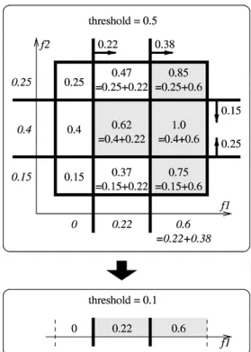
Figure 7. (top) A combination of a bounding box (the thick rectan-gle) and a boosted classifier, for two features f1and f2. Each plane
in the boosted classifier is a thick line with the positive half-space indicated by an arrow; the associated weightβis shown next to the arrow. The shaded area is the positive volume of the classifier, which are the pointsF wherekwk(fk) >1/2,k =1,2. The weights w1(·)andw2(·)are shown (in italics) along the f1- and f2-axes,
respectively, and the total weight w1(f1)+w2(f2) is shown for
each region of the bounding box. (bottom). The projected classifier, given byw1(f1) > 1/2−δ = 0.1 whereδ = maxf2w2(f2) =
max{0.25,0.4,0.15} =0.4.
assemblies are now used as negative data. A boosting algorithm (AdaBoost (Freund and Schapire, 1996)) is now applied to these negative assemblies and the origi-nal positive ones to learn a weighted committee of weak classifiers. The final classifier accepts an assembly if both the bounding box and the learned committee do so too. An example of a classifier is shown in Fig. 7(top).
Let F=(f1. . . fK) be the values of all features
computed for some complete assembly. The boosted classifier is learned as a weighted committee ofweak classifiers, each of which splits the feature space on a single feature. Thetth classifier (t =1. . .T) compares the value of thektth feature with some thresholdptand classifies an assembly as a person if
dt
fkt−pt
>0,
where dt ∈ {1,−1}determines which half-space is classified as positive.
The output of AdaBoost is a set of such weak classi-fiers (at each iteration of the algorithm, the feature fkt to split on, the thresholdptand the orientationdtof the separating plane are chosen so as to minimize the clas-sification error, which is computed as the sum of the weights of the misclassified data points, and the weights are updated at each iteration, assigning more weight to the points which have previously been misclassified). Additionally, AdaBoost will associate a weightβtwith each weak classifier; the resulting weighted committee will classify an assembly as positive iff
dt(fkt−pt) >0
βt >
dt(fkt−pt) <0
βt,
that is, if the total weight of the weak classifiers that classify the configuration as a person is greater than the weight of those classifying it as a non-person. By normalizing the weights so that tβt =1, we can rewrite the decision rule as
dt(fkt−pt) >0
βt >1/2.
The set{kt}may have repeating indices (that is, a feature may be split by several planes, which may have differentp,dandβvalues), and does not need to span the entire set 1. . .K.By grouping together the weights corresponding to planes splitting on the same feature, we rewrite the classifier as
K
k=1
wk(fk) >1/2, where
wk(fk)=
kt=k,dt(fk−pt) >0
βt
is the weight associated with the particular value of fea-ture fk. This weight is a piece-wise constant function of
fk; its points of discontinuity are given by{pt|kt =k}.
3.3.3. Projecting a Boosted Classifier. Given a
classifier constructed as above, we need to construct classifiers that depend on some identified subset of the features. Theprojected classifier Cl1...lk is a function of all those features that depend only on the seg-ments with labelsl1. . .lk and is used to separate sub-assemblies that could possibly be extended to a human
configuration from those that could not. In particular, if a complete assembly A can be formed by adding some label-segment pairs to A so that C(A) > 0,
thenCl1...lk(A) >0. The geometry of our classifiers—
whose positive regions consist of unions of axis-aligned bounding boxes—makes projection easy.
To obtain a projected classifier, one or more features—those that involve the segments left out by projection—must be projected away. For example, the projected classifier for assemblies consisting of a
torso
segment alone is obtained by keeping only the features that can be computed from thetorso
segment.
For convenience of notation, we show how to project away the feature fK; to project away several features, this process can be applied in a sequence to all of them. The idea that makes projection easy is that, since each weak classifier splits on a feature, projection will re-move those of them that split on fK, and will change the weights of the remaining classifiers in the committee.
The projection of the classifier should classify a point
Fin the(K−1)-dimensional feature subspace as pos-itive iff
max F
K
k=1
wk(fk) >1/2
whereFis a point in theK-dimensional feature space that projects to F but can have any value for fK. We can rewrite this expression as
K−1
k=1
wk(fk)+max
fK wK(f
K) >1/2.
The value of
δ =max
fK wK(f
K)
is readily available and independent of fK. We can see that, with the feature projected away, we obtain
K−1
k=1
wk(fk) >1/2−δ,
which has the same form as the original classifier, ex-cept that the threshold is no longer 1/2. Any number of features can be projected away in a sequence in this fashion. An example of the projected classifier is shown in Fig. 7(bottom).
3.3.4. Building Assemblies Incrementally. Assume
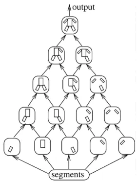
we have a classifierC that accepts assemblies corre-sponding to people and that we can construct projected classifiers as we need them. We will now show how to use them to construct assemblies, using apyramid of classifiers.
A pyramid of classifiers (Fig. 8), determined by the classifierCand a permutation of labels(l1. . .l9)
con-sists of nodesNli...lj corresponding to each of the pro-jected classifiersCli...lj,i ≤ j. Each of the bottom-level nodesNli receives the set of all segments in the image as the input. The top nodeNl1...l9outputs the set of all complete assembliesA= {(li,si) . . . (l9,s9)}such that
C(A) > 0, i.e. the set of all assemblies in the image
classified as people. Further, each nodeNli...lj outputs the set of all sub-assemblies A = {(li,si) . . . (lj,sj)} such thatCli...lj(A) >0.
The nodesNli at the bottom level work by selecting all segmentssi in the image for whichCli{li,si)}>0 (the only single-segment feature we use is the ratio of segment’s width to its length, so we simply select the segments with appropriate aspect ratios). Each of the remaining nodes has two parts:
Figure 8. A pyramid of classifiers. Each node outputs sub-assemblies accepted by the corresponding projected classifier. Each node except those in the bottom row works by forming assemblies from the outputs of its two children, and filtering the result using the corresponding projected classifier. The top node outputs the set of all complete assemblies that correspond to body configurations.
• Themergingstage of nodeNli...ljmerges the outputs of its children by computing the set of all assemblies {(li,si) . . . (lj,sj)}such that
Cli...lj−1{(li,si) . . . (lj−1,sj−1}>0 and
Cli−1...lj{(li+1,si+1) . . . (lj,sj)}>0. • Thefilteringstage then selects, from the resulting set
of assemblies, those for which
Cli...lj(·) >0,
and the resulting set is the output ofNli...lj.
Because C{(l1,s1) . . . (l9,s9)}>0 implies Cli...lj
{(li,si) . . . (lj,sj)}>0 for anyiand j, it is clear that
the output of the pyramid is, in fact, the set of all com-plete Afor whichC(A) >0 (note thatCl1...l9 =C, as a assembly is defined only by the set of segments and their labels but not their order).
The only constraint on the order in which the out-puts of nodes are computed is that children nodes have to be applied before parents. In our implementation, we use nodes Nli...lj where j changes from 1 to m, and, for each j,i changes from j down to 1. This is equivalent to computing sets of assemblies of the form
{(l1,s1) . . . (lj,sj)} in order, where getting (j +1)
-segment assemblies from j-segment ones is itself an incremental process, whereby we check labels against
lj+1in the orderlj,lj−1, . . . ,l1. In practice, we choose
the latter order on the fly for each increment step using a greedy algorithm, to minimize the size of assembly sets that are constructed (note that in this case the classifiers may no longer form a pyramid). The order(l1. . .l9)
in which labels are added to an assembly needs to be fixed. We determine this order off-line with a greedy algorithm by running a large segment set through the assembly builder and choosing the next label to add so as to minimize the number of assemblies that result.
3.3.5. Efficient Classification. The type of classifier
Cwe are using allows for an efficient building of assem-blies, in that the features do not need to be recomputed when we add a label-segment pair and move fromCl1...li toCl1...li+1.
We achieve this efficiency by carrying, along with an assembly A= {(l1,s1) . . . (li,si)}, the sum
σ (A)=
k∈K(l1...li)
wk(fk)
whereK(l1. . .li)is the set of all features computable from the segments labeled asl1, . . . ,li, and{fk}—the values of these features.
When we add another segment to get A= {(l1,s1)
. . . (li+1,si+1}, we can compute
σ (A)=σ(A)+
k∈K(l1...li+1)\K(l1...li)
wk(fk). In other words, when we add a labelli+1, we need to
compute only those features that require the segment
si+1for their computation.
4. Finding People by Sampling
The approach of Section 3 has the disadvantage of em-ploying a binary classifier, which tries to discriminate people from non-people. The problems with such a classifier include:
• Discrimination is made difficult by humans that ap-pear in unusual configurations or poses, have oc-cluded or low-contrast body parts, as well as by spu-rious limb-like segments that do not correspond to people but may, by chance, occur in groups that re-semble people.
• The classifier we described cannot determine how
likelyan assembly is to be a person, and thus makes it difficult to revise the classification if new infor-mation is added. For example, if two human-like as-semblies overlap each other, only one of them could represent the true configuration of a person, but the classifier will not be able to choose which assem-bly it is, since both of them are classified as people. This makes it difficult to count people, since a person often produces several human-like assemblies, and a subset of all assemblies must be chosen to determine how many people there are.
We address these problems by associating a likeli-hoodwith each assembly, which is proportional to the probability of seeing an assembly in a random view of a person and is high for the more human-like as-semblies and low for the non-human ones. Then, if we know that there is exactly one person in the image, we
may choose the maximum of the likelihood. To count people, we would count sufficiently separated peaks (modes). If the image is a frame in a video sequence, we may choose an assembly different from the likeli-hood mode if it agrees with the assemblies in the nearby frames—this could be used for robust tracking.
We represent the likelihood with a set of samples of assemblies, with probabilities of drawing an assembly proportional to its likelihood. As a result, the more an assembly looks like a person the more often it will be chosen, but assemblies that look less like people are not completely discarded, which will allow for incorpora-tion of future evidence (for example, in the counting procedure of Section 5.3).
To draw samples from the likelihood, we cannot use the brute-force method of computing the likelihood for each assembly, because of the huge number of possible assemblies. Instead, we propose to sample the likeli-hood by drawing samples from a sequence of approxi-mations, using resampling at each stage (cf. (Blake and Isard, 1998; Deutscher et al., 2000; Kanazawa et al., 1995; Neal, 1998)). In particular, we incrementally build segment groups ofincreasing size, by sampling them from appropriateintermediate distributions.
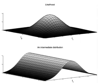
The intermediate distributions are derived from the likelihood so that, for a partial (<9-segment) assembly, the value of the corresponding intermediate distribution is high if it is likely that the assembly can be augmented to produce a human assembly, and low otherwise. This allows us to devote more attention to assemblies with a “higher potential.” The intermediate distributions make sampling from the likelihood possible, much like the projected classifiers of Section 3 help find assemblies accepted by the top-level classifiers, and the process of deriving them from the likelihood is quite similar to projection (see Fig. 9).
The samples from an intermediate distribution are augmented by adding a segment with a new label and
resamplingso as to get samples from the new interme-diate distribution. Usingimportance sampling, we are able to make sure that the incremental process of iter-ated resampling yields 9-segment assemblies that are, approximately, samples from the likelihood.
In this section, we explain why the likelihood makes sense, and show how to learn it from data. We show how to useimportance samplingto incrementally sam-ple assemblies of increasing size from the appropriate
intermediate distributions, so that at the end samples from the likelihood are obtained. The intermediate dis-tributions are not learned independently but aredirectly
Figure 9. The process of deriving intermediate distributions from the likelihood is quite similar to projection (cf. Fig. 6(b)). (top) The original likelihood depends on two features of an assembly: f1and
f2. (bottom). An intermediate distribution for assemblies for which
f2 cannot be computed (because these smaller assemblies do not
contain all of the segments on which f2depends).
derived from the likelihood, thus avoiding overfitting. We show how to count people in images, using the samples we obtain.
4.1. Sampling from Likelihood
We propose the probability of drawing an assembly as a sample to be proportional to its likelihood. The likelihood is defined as the probability density, in an appropriate feature space, of the set of features cor-responding to a 9-segment assembly, given that this assembly represents a person.
This density can be learned from data. Thus, the likelihood will favor assemblies that are, in some sense, similar to those in the training set. The model we use to learn the density is discussed in Section 4.3.2, but any other reasonable model could be used instead without changes to the general framework (a reasonable model is one that assigns a higher distribution value to an assembly that is more like a person).
The likelihood is an attractive distribution to sample from, since it is higher for the assemblies that are more people-like (according to the training set). It has to be noted that, although we refer to the likelihood as a
distribution, it is not really because the likelihoods of all assemblies in the image may not sum up to 1. The actual distribution we sample from is only proportional
to the likelihood; the constant of proportionality is hard to compute, but, fortunately, the sampling methods we use (importance sampling) do not need the distributions to be normalized.
Another justification for the use of likelihood is as follows. Suppose that we know that the segment set of an image contains exactly one 9-segment human as-sembly, and we need the posterior on which assembly it is. Assuming a uniform prior, we see that the posterior is
Pr[A=person|segments, 1 person] ∝L(A)
×P(segments| A=person,1 person)
(∝means proportional to). The first term of the right-hand side is the likelihood—how likely a random per-son is to look as the assembly A. The second term is the probability density of seeing the image segments, given that exactly one person, given by assembly A, is present. Assuming that segments are independent of one another, this is just the probability of seeing the segmentsnotinA. This probability doesn’t depend on the configuration ofA. We assume that the distribution on non-person segments is uniform; letαbe the value of the corresponding probability density. Then,
P(segments|A=person,1 person) ∝ P(segments not inA)
= α# segments not inA,
and the last term is the same for any 9-segment assem-bly A. Thus,
Pr[A=person|segments,1 person]∝ L(A),
and sampling from likelihood is the right thing to do.
4.2. Resampling
There are too many nine-segment assemblies to com-pute the likelihood for each. However, as in Section 3, we can build assemblies incrementally, and exclude smaller segment groups from further consideration if it can be determined that they cannot be a part of a person. For example, having generated a set of samples of the form{(
T
,sT)}of single-segment assemblies eachcon-sisting of a
torso
segment, and samples of the form {(LUA
,sLUA)}of assemblies each of which contains onlya
left upper arm
, we can form all combinations of the form{(T
,sT), (LUA
,sLUA)}and then resample those,so that the resulting samples of two-segment assem-blies {(
T
,sT), (LUA
,sLUA)}come from the appropriatemarginal likelihood or other appropriate intermediate distribution. (Presumably, among the resulting sam-ples, the groups similar to those found in people will occur more frequently.) We can proceed by similarly sampling 3-, 4-,. . . ,9-segment sub-assemblies, in such a way that the resulting set of 9-segment assemblies is sampled fromL(·).
At each stage, we useimportance sampling, which is a method for drawing samples from (possibly in-tractable) distributions (as used in (Blake and Isard, 1998)). In particular, to draw a sample from g(x), we first draw a large number of independent samples
{s1, . . . ,sn}from a proposal distributionf(x), and then
sets=siwith probability proportional towi = gf((xx)). As n → ∞, the distribution for the sample s will approachg(x). In our case, the proposal distribution
f(·)corresponds to theintermediate distribution Lkon
k-segment assemblies, while the target distributiong(·)
corresponds to the intermediate distribution Lk+1 on
(k+1)-segment assemblies. The intermediate distri-butions should be chosen in such a way that we are more likely to propose, for example, a two-segment assembly{(
RUA
,sRUA), (RLA
,sRLA)}if the two segmentsindividually are more likely to be
upper right arm
and
lower right arm
of a person; we discuss this choice in Section 4.3.4.4.3. Implementation
Our system starts by finding segments as described in Section 2. From the segments, we use a learned likeli-hood modelto formassembliesby sampling. To gener-ate assemblies, we use incremental sampling, whereby segment groups of increasing size are drawn from appropriateintermediate distributions, each of which roughly corresponds to a marginal likelihood but takes all image segments into account and is computed using dynamic programming. Finally, the set of assemblies is replaced with a smaller set ofrepresentatives, which are used to count people in the image.
By incrementally sampling segment groups of in-creasing size, we guide the sampler to larger assem-blies that are more human-like. Asymptotically (as the number of samples increases), the resulting samples of 9-segment assemblies will be drawn from the likeli-hoodL(A). Therefore, as in the method of Section 3, the intermediate distributions do not affect the final result; they do, however, help us obtain the samples fromL(A)more efficiently.
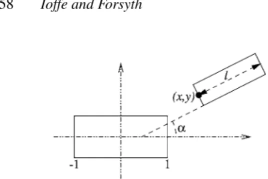
Figure 10. The parameterization of a joint. With one of the two segments, a frame of reference is associated, so that the coordinate axes are parallel to the sides of that rectangle, the origin is at its center, and all lengths are relative to the length of the segment (we scale the frame of reference so that the abscissae of the ends of the reference segment are 1 and−1). The 4 features that parameterize the joint are the coordinates(x,y)of the midpoint of the adjacent side of the second segment, the lengthlof the second segment (relative to that of the first), and the angleαbetween the segments.
4.3.1. Features. An assembly of 9 rectangular
segments, modulo rotation, translation and uniform scaling, has 41 degrees of freedom. A natural way to parameterize such an assembly is by a set of 9 aspect ratios, and 4 features at each of the 8 joints that encode the relative lengths, angles and displacements between adjacent segments (Fig. 10). Thus, each feature in our model depends on either one or two segments, and the two-segment features can be computed either from the two halves of the same limb (such as
right upper
arm
andright lower arm
), or from an upper limb and the torso.4.3.2. Learning Likelihoods for People. We assume
that the configurations at the joints are independent of one another. For example, the arms and legs can move almost independently of each other, and there is little correlation among the the configurations of the elbows and knees. We make the assumption for 3D configu-rations of people and extend it to their 2D projections onto the image plane. Another way of putting it in 2D is to say that, if we have several human assemblies, nor-malized so that, for example, the lengths and positions of their torsos are fixed, then by pasting together left arm of one of these assemblies, right leg of another, torso of the third, and so on, we will get another human assembly.
The main errors will be due to interactions between kinematic constraints on the hips and shoulders, and viewing pose. For instance, if we consider both frontal and lateral views of people, then the configuration of the torso and arms imposes constraints on the orientation of the person (frontal to lateral), which in turn constrains the configuration of the torso and legs.
While it is convenient to parameterize the body by independent joint configurations, we have found that such a model is not sufficient. Often, it results in assem-blies being found in the image such that several model segments are matched with the same image segment (e.g., a segment may be labeled as both the lower arm and upper leg). This causes the assemblies found for people to incorrectly represent their configuration, and also results in spurious non-human assemblies being classified as people (since, with coinciding segments, fewer than 9 segments are needed to build an assem-bly). We solve the problem by adding a constraint that all the segments in an assembly be distinct, and define the indicator functionIdist(A)to be 1 if this constraint is satisfied for assemblyA, and 0 otherwise. Then, we can write the likelihood from which we sample as
L(A)∝ Idist(A)×
41
k=1
k(fk), (1)
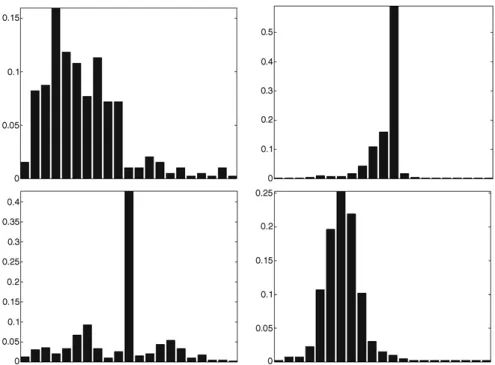
where fk is the value of the kth feature, and k(fk) is the corresponding one-dimensional marginal like-lihood. This representation avoids the problems with learning high-dimensional distributions: eachk(·)can be learned independently, from a relatively small data set. In our experiments, we chose fork(·)to be a his-togram for the values fk(Fig. 11).
Notice that while, without the Idist(A) term, our model could be described as a tree and dealt with using efficient inference methods available for tree-structured graphical models (such as dynamic pro-gramming (Felzenszwalb and Huttenlocher, 2000), it is no longer a tree. For example, the choices of segments corresponding to the left arm and the right arm are no longer conditionally independent given the torso. We will show, however, that dynamic programming could still be used to drive the search—namely, to compute the intermediate distributions from which sub-assemblies are drawn.
4.3.3. Building Assemblies Incrementally by
Resam-pling. We fix a permutation (l1, . . . ,l9) of labels
{
T
,LUA
, . . .}, and generate a sequence(S1, . . . ,S9)
of multisets (sets with possibly repeating elements) of samples, where each Sk contains N (not necessarily
Figure 11. Examples of histograms that are used to model one-dimensional distributionsiof features. Note the sharp spikes on some of the
histograms. They are due to the training data in which, for many limbs, a single segment was found, and thus the upper and lower halves had to be obtained by splitting this segment. This has biased our system towards such limb configurations.
distinct) assemblies of the form
l1,sl1
, . . . ,lk,slk
ofksegments labeled asl1, . . . ,lk(Fig. 12). For exam-ple, in our implementation,(l1. . .l9)=(
T
,LUA
,LLA
,. . .), and so S1 will contain the samples {(
T
,sT)} oftorso
segments, whileS3will contain samples{(
T
,sT), (LUA
,sLUA), (LLA
,sLLA)}of triples corresponding to the
torso
, theleft
up-per arm
and theleft lower arm
. The samples inSk are drawn from appropriately chosenintermediate
distributions Lk(·), discussed in Section 4.3.4. We generate the set of samples Sk+1fromSk using importance sampling. First, we form the set of sub-assemblies
l1,sl1
, . . . ,lk,slk
,lk+1,slk+1
for all groups
l1,sl1
, . . . ,lk,slk
∈Sk
Figure 12. We sample assemblies incrementally, by generating sets of samples of 1-, 2-,. . . ,9-segment assemblies, so that the latter are drawn from the likelihoodL(·). The setSkofk-segment assemblies
is drawn from the intermediate distributionsLk, withL9 = L. To
generate the setSk+1fromSk, we use importance resampling, with
resampling weights equal toLk+1(·)/Lk(·). Compare this to building
assemblies incrementally in the classification approach (cf. Fig. 8).
(which are assumed to be samples from Lk) and all choices ofslk+1. This way, we obtain samples of(k+1) -segment assemblies but which are drawn fromLkrather than Lk+1. We nowresamplethis set of samples, by
Figure 13. A tree-structured graphical model that could be used for human configurations if we lifted the constraint that all segments in an assembly be distinct. However, even for non-tree-shaped models, graphical models like this one can be used to drive the search, by allowing us to efficiently compute intermediate distributions for sub-assemblies that take into account all the image segments.
independently drawingNsamples, with the probability of drawing{(l1,sl1), . . . , (lk+1,slk+1)}proportional to
wl1,sl1
, . . . ,lk+1,slk+1
= Lk+1(·) Lk(·)
.
4.3.4. Intermediate Distributions. In the first
approximation, we could sample Sk by taking the corresponding intermediate distribution Lk to be the
marginal likelihood
Ll1...lk(A)∝ Idist(A)×
i
i(fi),
where the product is over all the features computable from segments labeled as l1, . . . ,lk, and Idist(A)=1 iff all of those segments are distinct, and =0 oth-erwise. We write sl for the segment of the sub-assembly whose label isl. For our feature set and the choice of(l1. . .l9), each of the marginal likelihoods
Ll1...lk(sl1, . . . ,slk)models the probability that the
sub-assembly(sl1, . . . ,slk)is seen in a random view of a human.
A disadvantage of using marginal likelihoods as in-termediate distributions is that the marginal likelihood of a sub-assembly does not depend on segments around it. For example, the value of such an intermediate distri-bution on a segment pair that looks like an arm will not depend on whether the segments around the pair look like the rest of a person or not. It would be desirable to be able to efficiently compute distributions that would take the sub-assembly’s context into account and pro-vide a better guide as to whether the sub-assembly is a part of a person.
If we can do this and find intermediate distributions that approximate
max{L(A)|Acontains the given subassembly},
then incremental sampling will sample complete assemblies from a distribution that better approximates
L(A). We believe this to be so because, when impor-tance sampling is used to sample from an unnormalized distributiong(·)via the intermediate distribution f(·), the target distribution is best approximated when the two distribution are proportional to each other.
When incrementally building assemblies, we add segments in the following order: the torso; the 4 up-per limbs; the 4 lower limbs. We will define, as our intermediate distributionsLk(·)onk-segment assem-blies, the maximum
max A⊃AL(A
)
over all the complete assemblies that contain the sub-assembly. When computing the maximum, welift the constraint that the same segment not be assigned sev-eral labels(so that now a segment can be, for example, left and right lower arm at the same time). By doing this, we ensure that all features computed for an assem-bly are computed from either single segments or pairs of adjacent segments, and thus the body model is tree-structured (Fig. 13). Indeed, all the numeric features described in Section 4.3.2 have this property; to com-pute intermediate distributions, we remove the binary feature for which this property does not hold: the fea-ture that is uniform if all the segments in an assembly are distinct, and is 0 otherwise.
The removal of the distinct-segments constraint is essential to making maximization efficient, since it re-duces the graphical model representing a person to a tree (with the torso as the root) for which efficient in-ference methods, such as dynamic programming, are available. On the other hand, this implies that the as-sembly Athus found may haveIdist(A)=0, and so we still need resampling steps to make sure that we sample fromL(A)rather than its relaxation.
The highest likelihood assembly, containing a given sub-assembly, is found by a simple Dynamic Program-ming algorithm, whereby we find the best lower half of a limb for each upper half, and then find the best limb of each type for each torso.
As an example, suppose that all of the segments in an assembly, except the lower left arm, are fixed, and we are to choose the lower left arm that maximizes the likelihood of the resulting assembly. It is easy to see that, in our model, the lower left arm can be found by considering all the pairs of a lower left arm (which can be any segment) and the upper left arm (which is fixed), and choosing the one with the highest marginal likelihoodLLUA,LLA. This is true because of the fact that
all features that involve the left lower arm may involve either no other segments or the left upper arm only.
Now, let us suppose that we have fixed a
torso
and, possibly, some limbs, and we want to add the left arm that would maximize the likelihood of the result. First, for each choicesLUAof the left upper arm, we will findthe best leftlowerarm
best
LLA(sLUA)by maximizingbest
LLA(sLUA)=arg max sLLA
LLUA,LLA{(
LUA
,sLUA), (LLA
,sLLA)}.Since no feature involves the left arm and any other limb, we can choose the best left arm for a given
torso
by considering all possible choices of the left upper
arm, each of which defines the whole arm as shown above. For a torso segment sT, we find the best left upper armbestLUA(sT)as follows:
best
LUA(sT)=arg max sLUALT,LUA,LLA
(T,sT),
(
LUA
,sLUA), (LLA
,best
LLA(sLUA))
.
Thus, for a torso segmentsT, the best left arm will be
{(
LUA
,best
LUA(sT)), (LLA
,best
LLA(best
LUA(sT)))}.Now we have an algorithm to compute max
A⊃AL(A
)
for any assemblyAwhich contains a torso segmentsT,
some whole limbs and some upper limbs—which, due to the order in which we add segments, is the only type of assemblies we deal with. For each of the 4 limbs, we do the following.
• If the whole limb is missing, add the best upper seg-ment
supper=
best
upper(sT)and the corresponding lower segment
slower=
best
lower(supper)=
best
lower(best
upper(sT)). • If just the lower half is missing, add the segmentslower=
best
lower(supper)that corresponds to the upper halfsupper.
This algorithm is efficient: because only pairs of segments are considered, it runs in O(n2)time forn
segments (and faster in practice, if we try to pair up only those segments that are close to each other). Al-though the upper bounds provided by this algorithm are very effective for directing the sampler to relevant image regions, they may not be tight. For example, in the resulting assemblies the legs may coincide. There-fore, the above algorithm does not replace sampling, but merely provides a good proposal mechanism.
Notice that a similar proposal mechanism could be used for any likelihood function L(A). To make use of efficient tree inference algorithms, we would sim-ply have to specify an approximationLtree(A)≈L(A) such that the modelLtreecould be represented as a tree-shaped graphical model, computed efficiently with dy-namic programming, and used to compute intermediate distributions.
5. Experiments
In this section, we describe the tests we used to ver-ify our methods. In Section 5.1, we describe the per-formance of the system described in Section 3, which learns a top-level classifier, and identifies all the im-age assemblies that are classified as people. To make the search efficient, assemblies are built incrementally, and non-human assemblies are rejected early by using projected classifiers, derived from the top-level one.
The results are encouraging but not quite satisfac-tory, in part because the system of Section 3 cannot count people. This suggests that it would be benefi-cial to have a measure of human-likeness associated with each assembly, and to retain some uncertainty