FEDERAL RESERVE BANK OF SAN FRANCISCO WORKING PAPER SERIES
The views in this paper are solely the responsibility of the authors and should not be interpreted as reflecting the views of the Federal Reserve Bank of San Francisco, the Federal Reserve Bank of New York, or the Board of Governors of the Federal Reserve System.
Working Paper 2014-12
http://www.frbsf.org/economic-research/publications/working-papers/wp2014-12.pdf
Has U.S. Monetary Policy Tracked the
Efficient Interest Rate?
Vasco CurdiaFederal Reserve Bank of San Francisco Andrea Ferrero
University of Oxford Ging Cee Ng University of Chicago
Andrea Tambalotti
Federal Reserve Bank of New York May 2014
Has U.S. Monetary Policy Tracked the Efficient Interest Rate?
IVasco C´urdiaa, Andrea Ferrerob, Ging Cee Ngc, Andrea Tambalottid,∗ May 8, 2014
aFederal Reserve Bank of San Francisco bUniversity of Oxford
cUniversity of Chicago dFederal Reserve Bank of New York
Abstract
Interest rate decisions by central banks are universally discussed in terms of Taylor rules, which describe policy rates as responding to inflation and some measure of the output gap.
We show that an alternative specification of the monetary policy reaction function, in which the interest rate tracks the evolution of a Wicksellian efficient rate of return as the primary
indicator of real activity, fits the U.S. data better than otherwise identical Taylor rules. This surprising result holds for a wide variety of specifications of the other ingredients of the
policy rule and of approaches to the measurement of the output gap. Moreover, it is robust across two different models of private agents’ behavior.
Keywords: U.S. monetary policy, Interest rate rules, DSGE models, Bayesian model
comparison
JEL Classification: E43, E58, C11
IWe thank Alejandro Justiniano, Robert King, Thomas Lubik, Ed Nelson, Giorgio Primiceri, Ricardo
Reis, Keith Sill, Chris Sims, and several seminar and conference participants for their comments. Matthew Hom provided excellent research assistance. The views expressed in this paper are those of the authors and do not necessarily reflect the position of the Federal Reserve Banks of New York or San Francisco, or the Federal Reserve System.
∗Corresponding Author: Federal Reserve Bank of New York, 33 Liberty Street, 3rd Floor, New York, NY
10045. Phone: (212) 720-5657; Fax: (212) 720-1844
Email addresses: [email protected](Vasco C´urdia),[email protected]
(Andrea Ferrero),[email protected](Ging Cee Ng),[email protected](Andrea Tambalotti)
1. Introduction
Interest rate rules are the tool of choice for economists and practitioners when describing
the conduct of monetary policy. Following Taylor (1993), these rules usually model the short-term interest rate as set in reaction to deviations of inflation from a target, and of
output from some measure of “potential.” A very large literature has shown that these two arguments, usually coupled with some inertia in the policy rate, provide an accurate
description of the observed evolution of the Federal Funds rate in the United States over the last several decades (e.g.,Judd and Rudebusch,1998; Clarida et al.,1999,2000;English
et al., 2003; Orphanides, 2003; Coibion and Gorodnichenko, 2011).
This paper proposes an alternative characterization of the factors influencing this
evo-lution. Our main finding is that policy rules in which the interest rate is set to track a measure of the efficient real rate—the real interest rate that would prevail if the economy
were perfectly competitive—fit the data better than rules in which the output gap is the primary measure of real economic activity. We refer to the former as W rules, from Knut
Wicksell (1898), who was the first to cast the problem of monetary policy as an attempt to track a “neutral” interest rate solely determined by real factors.1
To the best of our knowledge, we are the first to demonstrate the empirical plausibility of interest rate rules that respond to the efficient real rate.2 Although these rules have not been
previously examined in the empirical literature, the idea that a neutral, or “equilibrium”, interest rate might represent a useful reference point for monetary policy was familiar to
Federal Reserve policymakers well beforeWoodford(2003) revitalized its Wicksellian roots.3
For example, in his Humphrey Hawkins testimony to Congress in May 1993, Federal Reserve
1We do not call these rules Wicksellian because Woodford (2003) and Giannoni(2012) already use this
term to refer to interest rate rules that respond to the price level, rather than to inflation.
2Trehan and Wu(2007) discuss the biases in the reduced-form estimation of policy rules with a constant
intercept, when in fact the central bank responds to a time-varying equilibrium real rate, but they do not estimate this response.
3King and Wolman (1999) were the first to show that, in a New Keynesian model, it is optimal for the
Chairman Alan Greenspan stated that
“...In assessing real rates, the central issue is their relationship to an equilib-rium interest rate, specifically, the real rate level that, if maintained, would keep
the economy at its production potential over time. Rates persisting above that level, history tells us, tend to be associated with slack, disinflation, and economic
stagnation—below that level with eventual resource bottlenecks and rising infla-tion, which ultimately engenders economic contraction. Maintaining the real
rate around its equilibrium level should have a stabilizing effect on the economy, directing production toward its long-term potential.”4
Evaluating the extent to which Greenspan’s reasoning had a measurable impact on the ob-served evolution of policy rates in the U.S. requires a structural model, since the equilibrium
real rate he describes is a counterfactual object. We compute this counterfactual within two variants of the standard New Keynesian DSGE model with monopolistic competition
and sticky prices, estimated on data for the Federal Funds rate (FFR), inflation and GDP growth, as in the empirical literature on Taylor rules.
Given this framework, we follow Greenspan’s qualitative description of the equilibrium interest rate and compute the counterfactual “real rate level that, if maintained, would keep
the economy at its production potential over time.” If we define “production potential” as the efficient level of aggregate output ye
t, as in Justiniano et al. (2011) for instance, the equilibrium real rate corresponds to the efficient rate of return ret. This interest rate is efficient because it is the one that would prevail if markets were perfectly competitive, rather
than distorted by monopoly power and price dispersion.
Our exploration of the fit of W rules starts from a very simple specification, in which the
4Quantitative measures of this equilibrium interest rate are a regular input in the monetary policy debate
at the Federal Reserve. A chart with a range of estimates of this rate is included in most published Bluebooks at least since May 2001. According to McCallum and Nelson (2011), this construct emerged in the early 1990s at the Federal Reserve as a gauge of the monetary policy stance following a shift of emphasis away from monetary aggregates, due to the difficulty of estimating a non-inflationary growth rate of money in the midst of financial innovation. See alsoAmato(2005).
FFR closes the gap with re
t over time, and responds to inflation, as in
it=ρit−1+ (1−ρ) (rte+φππt) +εit.
We compare the empirical performance of this baseline W rule with that of a more traditional
T rule based on Taylor (1993), in which economic slack is measured by the output gap. The model’s ability to fit the data deteriorates significantly under the latter specification.
We then illustrate the robustness of this surprising finding to several variations in the other ingredients of the policy rule—including the measurement of the output gap, and the presence
of a time-varying inflation target—as well as in the specification of the rest of the DSGE model.
Methodologically, we follow a full-information, Bayesian empirical strategy. First, we couple each of the policy rules whose fit we wish to evaluate with the private sector’s tastes
and technology described by the DSGE model. This step results in a set of econometric models, one for each policy specification. Second, we estimate all these models and compare
their fit using marginal data densities.5
This criterion measures each model’s overall ability to fit the data, rather than that of
the policy equation alone, relative to a reference model, which in our case is that associated with the W rule. This is the only formal approach to evaluating fit in the general equilibrium
context called for by the need to compute the counterfactual efficient real rate. However, we also complement this approach with some more informal indicators of how well different
policy rules account for the evolution of the FFR, and of the extent to which the resulting model is more or less sensible.
Aside from pointing to W rules as a promising tool to describe interest rate setting in practice, our exploration of the fit of many of the policy specifications used in DSGE and
other applied work in monetary economics suggests that this often neglected component of structural models can have a significant impact on their fit. The gap in marginal likelihoods
5An and Schorfheide(2007) provide a comprehensive survey of the application of Bayesian methods to the
estimation and comparison of DSGE models. Lubik and Schorfheide(2007) use similar methods to estimate the response of monetary policy to exchange rate movements in several small open economies.
between the best and worst fitting rules included in this study can be as high as fifty
log-points. As a reference, these differences in fit are of a similar order of magnitude as those between structural models estimated with or without stochastic volatility found by C´urdia
et al. (2011). This evidence therefore underscores the importance for DSGE researchers of paying significantly more attention to the specification of monetary policy than common so
far.
The rest of the paper proceeds as follows. Section2presents our baseline model of private sector behavior, defines its efficient equilibrium and the associated levels of output and of
the real interest rate, and introduces the baseline W and T rules. Section 3 discusses the methodology for the estimation and comparison of the models. Section 4 presents results
for the baseline policy rules, making the case for the empirical superiority of the W rule. Section5explores the robustness of this conclusion to alternative specifications of the policy
rules, and of the private sector’s tastes and technology. Section 6 concludes. An online Appendix contains a larger set of robustness results, along with a more detailed description
of the baseline model and other supporting material.
2. A Simple Model of the Monetary Transmission Mechanism
This section outlines the log-linear approximation of the simple New-Keynesian model we bring to the data. The model describes the behavior of households and firms, with an interest
rate feedback rule capturing the response of monetary policy to economic developments. Different specifications of this reaction function, coupled with the same tastes and technology
for the private sector, give rise to different empirical models. Details on the microfoundations are in the online Appendix.
An intertemporal Euler equation and a Phillips curve summarize the behavior of the private sector. Optimal consumption and saving decisions produce the Euler equation
˜
xt=Etx˜t+1−ϕ−γ1(it−Etπt+1−rte), (1) which states that current real activity, measured by the variable ˜xt ≡ (xet − ηγxet−1) −
ex-ante real interest rate,it−Etπt+1, and its efficient level ret. Here,itis the nominal interest rate, πt is inflation, and xet ≡ yt−yte is the efficient output gap, i.e. the log-deviation of output,yt from its efficient level yet.
The optimal pricing decisions of firms produce the Phillips curve
˜
πt =ξ(ωxet +ϕγx˜t) +βEtπ˜t+1+ut, (2)
relating a measure of current inflation, ˜πt ≡ πt−ζπt−1, to expected future inflation, real
activity and an AR(1) cost-push shock ut, generated by exogenous fluctuations in desired
markups.
These two equations augment the purely forward-looking textbook version of the New
Keynesian model with two sources of inertia, which improve its ability to fit the data. On the demand side, utility features internal habits in consumption, parametrized by ηγ. On
the supply side, the prices that are not re-optimized in each period increase automatically with past inflation, by a proportion ζ.
This model of private sector behavior is more stylized than in the workhorse empirical DSGE framework ofChristiano et al.(2005) andSmets and Wouters(2007). In particular, it
abstracts from capital accumulation and the attending frictions (endogenous utilization and investment adjustment costs) and from non-competitive features in the labor market
(mo-nopolistic competition and sticky wages). Nevertheless, it provides a reasonable description of the data on GDP, inflation and the interest rate—the series that are typically considered
in the estimation of interest rate rules. Another advantage of working with a stripped-down baseline specification is that it made it possible to explore the robustness of the paper’s main
finding across a very large number of interest rate rules, without having to worry about com-putational constraints. Nevertheless, section 5.3shows that W rules also outperform T rules
in a medium-scale model.
2.1. Output and the Real Interest Rate in the Efficient Equilibrium
Efficient output, denoted by ye
t, and the efficient real interest rate, denoted by rte, are central constructs in our analysis. They represent the levels of output and of the real
interest rate that would be observed in a counterfactual economy in which (i) prices are—
and have always been—flexible, and (ii) desired markups are zero. In our framework, these assumptions result in a perfectly competitive economy, which would therefore deliver the
efficient allocation. The corresponding equilibrium represents a “parallel universe”, which evolves independently from the outcomes observed in the actual economy (Neiss and Nelson,
2003).
In this parallel universe, efficient output, expressed in deviation from the balanced growth path, evolves according to
ωyte+ϕγ(yet −ηγyte−1)−βϕγηγ(Etyte+1−ηγyte) = ϕγηγ(βEtγt+1−γt) +
βηγ 1−βηγ
Etδt+1. (3)
This equation implies that ye
t is a linear combination of past, current, and future expected values of productivity growth γt and of the intertemporal taste shock δt. These exogenous
disturbances both follow AR(1) processes. Given ye
t, the intertemporal Euler equation implies
ret =Etγt+1+Etδt+1−ωEt∆yet+1, (4)
from which we observe that the efficient real rate depends positively on the forecastable
components of next period’s productivity growth and preference shock, and negatively on those of the growth rate of efficient output, ∆ye
t+1. Intuitively, an increase in households’
desire to consume early, which is captured by a persistent rise inδt,puts upward pressure on the efficient real rate, so as to dissuade consumers from acting on their desire to anticipate
consumption. Similarly, higher expected productivity growth requires steeper consumption profiles, and hence a higher real rate. Finally, the last term captures the negative effect on
the interest rate of a higher expected growth rate of marginal utility, which in the efficient equilibrium is connected with the growth rate of hours, and hence of output.
These last two expressions highlight the close connection between the efficient levels of output and of the real rate, while Euler equation (1) ties together their respective gaps.
According to (1), an interest rate gap maintained at zero forever closes the output gap, and vice versa. This observation suggests that re
alternative to the efficient level of output, as an indicator of the economy’s potential. In
the context of policy rules, this alternative approach to assessing the amount of slack in the economy can be captured by an interest rate that tracks its efficient counter part, as in the
W rules presented below.
2.2. Monetary Policy: Baseline W and T Rules
To set up the comparison between policy rules that track the efficient real rate, or W
rules, and those that react to the output gap instead, or T rules, we begin our analysis with two particularly simple specifications.
In the baseline W rule, the policy rate responds to the efficient real rate and to inflation, with some inertia, as in
it=ρit−1+ (1−ρ) (rte+φππt) +εit. (5) The coefficient on re
t is restricted to one because this indicator represents a target for the actual interest rate. When the efficient rate rises, say because of an increase in households’ desire to consume today, the actual rate follows, so as to close the interest rate gap, and
hence keep output close to its efficient level.
In the baseline T rule, the central bank sets the nominal interest rate in response to
inflation and the efficient output gap
it=ρit−1 + (1−ρ) (φππt+φxxet) +ε i
t. (6)
In this case, demand pressures are captured by the deviation of output from its efficient level, to which the central bank reacts by increasing the policy rate.
Therefore, both baseline rules capture the typical reaction of monetary policy to real economic developments. In the W rule, these developments are summarized by the efficient
real rate. In the T rule, they are captured by the output gap.
To bridge the gap between the empirical literature on interest rate rules and this paper’s
DSGE framework, equation (6) defines the output gap as the deviation of output from its efficient level. This choice, which might be controversial, is dictated by two considerations.
inflation and the measure of slack that is relevant for welfare (e.g. Woodford,2003). Second,
the efficient output gap is a direct counterpart to the efficient real interest rate that measures economic activity in the baseline W rule.
The main drawback of this modeling choice is that computingxe
t requires a fully-specified model, while most of the measures featured in the empirical literature do not. For this reason,
we later extend the comparison between W and T rules to specifications that include other
definitions of the output gap, such as ones based on the HP and other statistical filters. As we pointed out in the previous section, if monetary policy ensured thatit−Etπt+1 =ret in every period, the output gap would always be zero and aggregate output would never deviate from its efficient level. But if this is the case, why include inflation in the W rules?
The main reason is that with output at its efficient level, cost-push shocks pass-through to inflation entirely, as we can see by solving equation (2) forward with yt=yte, ∀t
πt=ζπt−1 +
∞
X
s=0
βsEtut+s.
The resulting fluctuations in inflation produce inefficient dispersion of prices and production levels across goods varieties, even if aggregate output is at its efficient level, making this
pol-icy undesirable. At the other extreme, perfect inflation stabilization causes cost-push shocks to show-through entirely in deviations of output from its efficient level, which is also
sub-optimal.6 Optimal policy, therefore, distributes the impact of these shocks between output and inflation, balancing the objectives of price stability and efficient aggregate production.
The W rule mimics this trade-off by including an inflation term, just like T rules do.7
6Woodford (2003) calls “natural” the levels of output and of the real interest rate observed in this
equilibrium with stable inflation. Barsky et al.(forthcoming) discuss the relationship between natural and efficient equilibria in New Keynesian models and the neutral rate of interest inWicksell (1898). Justiniano et al.(2011) connect these concepts to optimal policy.
7Another reason why i
t =ret +Etπt+1 is not a viable policy rule is that it does not satisfy the Taylor
3. Inference
We estimate the two alternative models associated with the W and T rules laid out
in the previous section—and the many variants discussed below—with Bayesian methods, as surveyed for example by An and Schorfheide (2007). Bayesian estimation combines prior
information on the model’s parameters with its likelihood function to form a posterior density, from which we draw using Markov Chain Monte Carlo (MCMC) methods. We construct
the likelihood using the Kalman filter based on the state-space representation of the rational expectations solution of each model under consideration, setting to zero the prior probability
of the configurations of parameters that imply indeterminacy. The observation equations are
∆ logGDPt = γ+yt−yt−1+γt ∆ logP CEt = π∗+πt
F F Rt = r+π∗+it,
where GDPt is real GDP, P CEt is the core PCE deflator (ex-food and energy), and F F Rt
is the average effective Federal Funds Rate (henceforth FFR), all sampled at a quarterly fre-quency. The constants in these equations represent the average growth rate of productivity
(γ), the long run inflation target (π∗), and the average real interest rate (r). The sample pe-riod runs from 1987:Q3 to 2009:Q3, although the main results are not affected by truncating
the sample either at 2008:Q4, when the FFR first hit the zero bound, or at 2006:Q4, before the eruption of the recent financial crisis. We start the sample on the date in which Alan
Greenspan became chairman of the Federal Reserve because this period is characterized by a reasonably homogenous approach to monetary policy, which is well-approximated by a
stable interest rate rule.
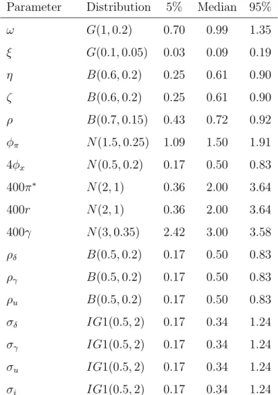
Table 1reports our choice of priors, which are shared across all the models we estimate.
On the demand side, we calibrate the discount factor asβ = 0.99. This parameter, together with the balanced growth rate γ, and the habit coefficient η, determines the slope of the
On the supply side, the slope of the Phillips curve is also a function of deep parameters,
ξ = (1−α) (1−αβ)/[α(1 +ωθ)], where α is the fraction of firms that do not change their price in any given period, θ is the elasticity of demand faced by each monopolistic producer
and ωis the inverse Frisch elasticity of labor supply. Given our observables, only the slopeξ
can be identified. Its prior, centered around 0.1, is somewhat higher than typical estimates
of the New Keynesian Phillips curve (e.g. Gal´ı and Gertler, 2007; Sbordone, 2002), but
consistent with the low degree of price stickiness found in microeconomic studies such as Bils and Klenow (2004), given reasonable values forω and θ.8
In the interest rate rules, the prior on the smoothing parameter ρ has a dispersion wide enough to encompass most existing estimates. The priors for the feedback coefficients on
inflation φπ and real activity φx are centered around the original Taylor (1993) values of 1.5 and 0.5, respectively.
To evaluate the fit of different policy rules, we compare the marginal data densities (or posterior probabilities) of the corresponding models. All these models share equations (1) and
(2), but each is closed with a different interest rate rule. We estimate each model separately with the same data and priors, and compute its posterior probability using the modified
harmonic mean estimator proposed by Geweke (1999). To compare fit across models, we calculate KR ratios, defined as two times the log of the Bayes factor.9 Kass and Raftery
(1995) recommend this measure of relative fit since its scale is the same as that of a classic Likelihood Ratio statistic. They suggest that values of KR above 10 can be considered “very
strong” evidence in favor of a model. Values between 6 and 10 represent “strong” evidence, between 2 and 6 “positive” evidence, while values below 2 are “not worth more than a bare
mention.”
8For example, with ω = 1 and θ = 8, which corresponds to a desired markup of 14%, ξ = 0.1 implies
α= 0.4,or an expected duration of prices of about five months.
4. Results: Wicksell or Taylor?
This section illustrates the central result of the paper: the baseline W rule fits the
data better than its T counterpart. Subsequent sections demonstrate that the superior empirical performance of W rules extends well beyond the baseline specification and remains
remarkably robust across dozens of variations on the ingredients of the rule, as well as in a richer DSGE model. To the best of our knowledge, we are the first to document the excellent
performance of W rules as tools to describe observed monetary policy behavior.
Table 2 reports the posterior estimates of the parameters under the two baseline policy
specifications, together with the models’ marginal likelihoods and the implied KR criterion. The table conveys the excellent empirical performance of the W rule along three dimensions.
First, the nearly eleven point difference in log-marginal likelihoods between the two models translates into a KR ratio above 20, which represents very strong evidence in favor of the
model featuring the W rule. This is the most formal and reliable piece of evidence in favor of this policy specification.
Second, the posterior estimates of the parameters support this evidence and provide some insight into the empirical difficulties of the baseline T specification. For instance, the
posterior of the slope of the Phillips curveξ is concentrated near extremely low values under this specification, with a median of 0.0021. This value is two orders of magnitude smaller
than the prior mean and at the extreme lower end of the available estimates in the DSGE literature (see, for example, the survey bySchorfheide, 2008).
A coefficient this low implies no discernible trade-off between inflation and real activity,
so that inflation is close to an exogenous process driven by movements in desired markups. As a consequence, it becomes hard to distinguish between inflation indexation and persistent
markup shocks as drivers of the observed inflation persistence. This lack of identification is reflected in bimodal posterior distributions of the parametersζ and ρu,which are generated
by MCMC draws with high ζ and low ρu, or vice versa, as shown in Appendix C. These draws correspond to local peaks of the joint posterior density of similar heights.
Finally, the interest rate rule coefficients imply a fairly strong reaction of policy to the output gap, but an extremely weak reaction to inflation, with a substantial fraction of the
posterior draws forφπ below one. These values are at odds with the large empirical literature
that has found a forceful reaction to inflation to be one of the hallmarks of U.S. monetary policy since the mid-eighties.10 None of these problems appears in the model with the W
rule, from which we conclude that this specification also provides a more sensible description of the data.
The two indicators of the empirical plausibility of the W rule considered so far speak to
the overall model’s ability to account for the evolution of the entire vector of observables, rather than pointing to the success of the policy specification by itself. The last evaluation
criterion we consider, therefore, focuses more narrowly on the extent to which the systematic component of the policy rule accounts for the observed movements in the FFR, in the spirit
of the R2 in a regression.
Unfortunately, we are not aware of any formal approach to evaluating the fit of an
individual equation in a DSGE model estimated with full-information methods. As an impressionistic alternative, the third row of Table 2 reports the standard deviation of the
smoothed sequence of monetary policy shocks in each specification, denoted by Std(εit|T). This statistic measures the observed variation in the FFR left unexplained by the feedback
component of the policy rule. It is the “sample analog” of the posterior estimate of the standard deviation of the monetary policy shock,σi, and is usually very close to the median
of its posterior.
This standard deviation is 29 basis points for the W rule and 30 basis points for the T
rule, a minor difference. However, the difference is larger (25 basis points for the W rule compared to 32 for the T rule) if we drop from the sample the recent recession, in which
the nominal interest rate has fallen to its zero lower bound. This evidence suggests that in “normal” times the W rule accounts more closely for the systematic behavior of interest
rates than the T rule. This advantage diminishes when a deep downturn drives the efficient interest rate well below the zero lower bound, as it did in the Great Recession.
10Values of φ
π lower than one do not necessarily generate indeterminacy, if accompanied by high values of φx. Equilibrium is determinate in the baseline model if and only if φπ+ (1−β)φx/ξ >1,as shown by
4.1. Wicksell and Taylor
As pointed out in Section 2.1, our simple baseline model implies that an actual real rate that always matches its efficient counterpart ultimately closes the output gap, and vice versa.
Therefore, these two approaches to stabilizing the real economy—closing the output or the interest rate gap—might be useful complements. To explore this possibility, we estimated a
model with a combined W&T rule of the form
it=ρit−1+ (1−ρ) [rte+φππt+φxxet] +ε i
t. (7)
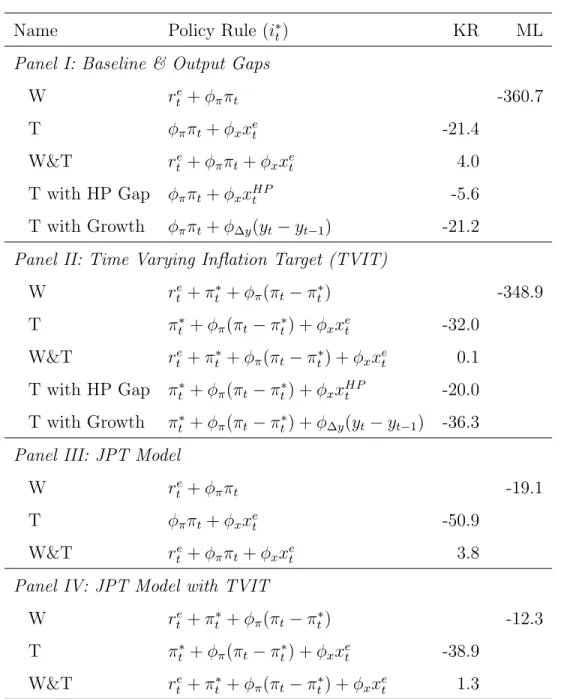
This specification yields a modest improvement in fit over the baseline W rule of 4 KR points, as shown in the first panel of Table 3. This improvement represents positive
evidence that both the efficient real rate and the output gap contain useful information for policymakers on the state of the real economy. However, the much larger improvement in
fit obtained by substituting xet with ret (21.4 KR points moving from the T rule to the W rule), as compared to adding xe
t to rte (4 KR points moving from the W rule to the W&T rule), suggests that the latter is by far the most useful real indicator between the two. In fact, the performance of the W&T rule is actually inferior to that of the W rule in several
of the alternative specifications considered in the robustness exercises, further strengthening the conclusion.
4.2. Estimates of the Efficient Real Rate and of the Output Gap
The evidence presented so far points to the efficient real rate as a crucial indicator for
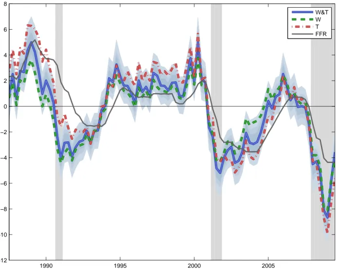
monetary policy. Figure 1 illustrates its estimated behavior over time. It plots smoothed posterior estimates of re
t under the W, T and W&T models, along with the effective FFR. This picture drives home three important points.
First, the estimated efficient real interest rate is a good business cycle indicator, rising
during booms and dropping sharply in recessions. In fact, the efficient real interest rate conveys early signals of the upcoming slowdown in all three recessions in our sample, dropping
sharply a few quarters before the recession actually starts, ahead of the turning point in the FFR. Second, the inferred movements in re
t mirror quite closely those in the FFR, which helps explain the empirical success of W rules.
The close co-movement between the FFR and the estimates of re
t may raise the concern that the observations on the nominal interest rate “explain” the estimates ofre
t, and not vice versa. However, this is not the case, which is the third important message of the figure. In
fact, the estimated time path of re
t in the two models whose policy rules include it (W and W&T) is very close to that under the T specification, in whichre
t does not affect interest rate setting. The main difference among the estimates is that the posterior distribution is tighter
when ret enters the interest rate rule, as in the bands for the W&T specification shown in the figure. This enhanced precision of the estimates suggests that the nominal interest rate
does carry useful information on ret, as should be expected, but that this information does not distort the inference on its median time-path.
Some intuition for the remarkable consistency of the estimates ofrteacross models can be gleaned from the expression for the efficient real interest rate presented in section 2, which
we report here for convenience
rte =Etγt+1+Etδt+1−ω Et∆yet+1
.
If efficient output growth were not expected to deviate from the balanced growth path (i.e. Et∆yte+1 = 0), the efficient real interest rate would be the sum of the forecastable
movements in the growth rate of productivityγt and in the intertemporal taste shock δt. In the estimated models, Et∆yet+1 is indeed close to zero and the forecastable movements in γt
are small. The taste shockδt, on the contrary, is large and persistent, so that its movements tend to be the main driving force of re
t. These movements are pinned down quite precisely by the estimation procedure, making the inference on the evolution of the efficient real rate remarkably consistent across models. In fact, this consistency extends well beyond the three
specifications depicted in figure 1to virtually all the models considered in the robustness exercises, as illustrated in Appendix F.
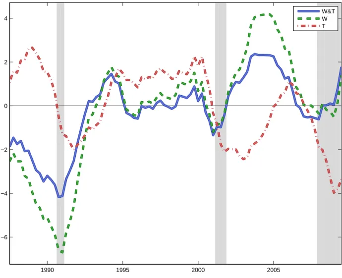
We conclude this section by looking at the estimated output gap. This exercise is an important reality check on the baseline results, since one might wonder if the baseline T rule
does not fit because it forces the interest rate to respond to an unreasonable gap measure. Figure 2 shows that this is not the case. In fact, the efficient output gap obtained under
views on the evolution of economic slack over the sample. Unlike with the estimates of re t reported in Figure1, though, inference on the output gap is sensitive to the monetary policy specification. Under the W and W&T rule, the output gap is less clearly cyclical than in the
T specification, which makes it a less reliable indicator of real activity than the efficient real rate. This conclusion is further supported by the robustness analysis conducted in the next
section, which shows that the superiority of the W rule survives many alternative approaches
to measuring the output gap included in the T rule.
5. Robustness
The comparison between the baseline W and T rules conducted so far suggests that the efficient interest rate captures the real economic developments to which the Federal Reserve
has responded over the past twenty five years better than the efficient output gap. This section demonstrates that this result does not depend on the arbitrary choice of the baseline
policy specifications. Regardless of how we measure the output gap, or of how we choose the other arguments of the policy function, W rules always fit the data better than comparable
T rules. Moreover, this result remains true within a medium-scale DSGE model, along the lines of Christiano et al. (2005) and Smets and Wouters (2007).
5.1. Output Gap
The measure of the output gap included in the baseline T rule is the deviation of real GDP from its efficient level. This choice is fairly common in DSGE work (Smets and Wouters,
2007, e.g.), but it is not without controversy in the broader macroeconomic literature, since efficient output can only be computed within a fully specified model. In fact, Taylor rules
became so successful partly because they could be estimated without taking such a specific stance on how to measure economic slack, nor on the rest of the model.
To bridge the gap between our general equilibrium framework and the empirical work based on single equation methods, we examined several statistical approaches to the
con-struction of smooth versions of potential output. In this section, we focus on one such approach, the Hodrick and Prescott (HP) filter, given its popularity in applied
macroeco-nomics.11 The Appendix includes a discussion of our general approach to filtering within
DSGE models, as well as results for several other filters we experimented with.
To make the HP filter operational within the DSGE framework, we adapt the
methodol-ogy proposed by Christiano and Fitzgerald(2003) for the approximation of ideal band pass filters. These authors use forecasts and backcasts from an auxiliary time-series model—in
their case a simple unit root process—to extend the available vector of observations into the
infinite past and future. They then apply the ideal filter to this extended sample. In our implementation of their idea, the auxiliary model that generates the past and future dummy
observations is the linearized DSGE itself.
This approach is particularly convenient because it produces a very parsimonious
recur-sive expression for what we call the DSGE-HP gap xHPt
1 +λ(1−L)2(1−F)2xHPt =λ(1−L)2(1−F)2yt, (8) where the operatorsLandF are defined byLyt=yt−1 andF yt =Etyt+1, and the smoothing
parameterλ is set at the typical quarterly value of 1600. This expression can thus be added to the system of rational expectations equations that defines the equilibrium of the model
without dramatically augmenting the dimension of its state vector.12
When we estimate the model with a T rule in whichxHP
t replaces the efficient output gap, the fit improves significantly compared to the baseline T specification (about 15 KR points). However, it remains below that of the baseline W rule by close to 6 points, as shown at the
bottom of panel I in Table 3. This difference in fit between the W rule and the T rule with the HP output gap is fairly small in the baseline specification. However, in the next section
we show that the difference becomes much larger (20 KR points) in the specifications with a time-varying inflation target, which further improves the fit of the model. Overall, these
11See Orphanides and Van Norden (2002) for a comprehensive survey of the use of statistical filters as
measures of the output gap and their pitfalls.
12The time series for the output gap obtained through this procedure (DSGE-HP) is very similar to that
produced by the standard finite sample approximation of the HP filter applied to the GDP data. This result supports our use of the DSGE-HP filter as an effective detrending tool, which produces a measure of economic slack similar to those often used in single-equation estimates of the Taylor rule.
results confirm that the superior empirical performance of W over T rules is not sensitive to
the measurement of the output gap.
To further substantiate this conclusion, the Appendix reports the fit of several alternative
models in which the output gap in the T rule is measured with a variety of other filters. None of these alternative measures of the output gap helps the model fit better than the DSGE-HP
gap described above. As an example, panel II of Table3considers the simplest among these
alternative filters: the quarterly growth rate of output, which is a fairly common choice in estimated DSGEs. The performance of this T rule is in line with that of the baseline T
specification, and hence it is substantially worse than that of the baseline W rule.
5.2. Time-Varying Inflation Target
In this section, we modify the baseline policy specification by introducing a time-varying inflation target (TVIT). This is a common feature in the recent empirical DSGE literature,
which helps capture the low-frequency movements in inflation and the nominal interest rate that are evident even in our relatively short sample (G¨urkaynak et al., 2005; Ireland, 2007;
Cogley et al., 2010; Del Negro and Eusepi, 2011; Del Negro et al., 2013). This addition creates a new class of feedback rules, whose W&T version is
it=ρit−1 + (1−ρ) [rte+π ∗
t +φπ(πt−πt∗) +φxxt] +εit, (9)
where π∗t is an exogenous AR(1) process representing persistent deviations of the inflation
target from its long-run value π∗.13 The corresponding W rule has φx = 0, while the T rule does not include re
t.
The inclusion of a TVIT significantly improves the fit of the W model, as shown in panel II of Table 3. Its KR ratio with respect to the baseline W specification is around 24 points,
very strong evidence in favor of the inclusion of this element in the policy rule. However, the TVIT does not have an equally positive effect on the performance of the other specifications.
As a result, the gap between the W rule and its competitors is even larger in this panel than in the previous one. Among these competitors, the T rule with the HP output gap continues
13The autocorrelation coefficient ofπ∗
to outperform the one with xe
t, but it is 20 KR points below the W rule. Moreover, the W&T rule does not improve over the W rule, unlike in the baseline case.
These results suggest that the efficient real rate and a smoothly evolving inflation target
enhance the empirical performance of the model through fairly independent channels. The former helps improve the business cycle properties of the model, while the latter helps capture
the low frequency component of inflation, making them complementary features in policy
specifications with good empirical properties.
5.3. A Medium-Scale DSGE Model
We conclude our investigation of interest rate rules by extending the comparison of W and T rules to a medium-scale DSGE model, along the lines ofChristiano et al. (2005) and
Smets and Wouters(2007). The exact specification we adopt for the behavior of the private sector behavior follows Justiniano et al. (2010) (henceforth, JPT), to which we refer the
reader for further details. To make the exercise more directly comparable to that conducted in the baseline model, we estimate the JPT model on the same set of observables—GDP
growth, inflation and the FFR—and on the same sample.
Panels III and IV of Table 3 report the results, which are even more strongly in favor
of the W rule. First, the improvement in fit of the W over the T rule is 51 KR points, the largest among all the models we considered. Second, adding the output gap to the W rule
to form the W&T specification brings a further improvement, which is however very small. Also in this model, therefore, the efficient real rate is by far the most effective measure of real
economic developments from the perspective of monetary policy. Third, the introduction of a TVIT improves the model’s fit, but it leaves intact the superiority of the W rule, which
now amounts to 39 KR points over the T rule.
To put these differences in fit in perspective,C´urdia et al.(2011) report that the inclusion
of stochastic volatility within a DSGE structure very similar to that of JPT improves their model’s fit by about 68 KR points. This consideration suggests that choosing an
appropri-ate policy specification can yield comparable gains in fit as correctly specifying its driving processes, which are widely regarded as crucial to the empirical success of these models.
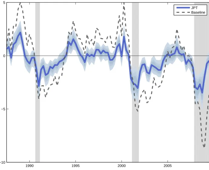
Finally, Figure3compares the estimated time series ofre
t in the baseline and JPT models under the W&T policy rule. We chose this specification because it is the best fitting one, but very similar results hold for the baseline W rule, as well as for the W&T and W rules with
a time varying inflation target. The estimated efficient rate retains the cyclical properties stressed in section4.2 also in the JPT model, although its fluctuations are more muted than
in the baseline. This reduction in estimated volatility is probably due to the richer set of
frictions (and shocks) included by JPT, which account for some of the movement in the data through endogenous propagation and amplification channels omitted from the baseline
model. These channels reduce the role of the intertemporal shock δt,which is the key driver of the efficient rate in that model. We conclude that the estimates of the efficient real rate
are at least qualitatively robust to major changes in the model, as well as to changes in the policy specification, as also illustrated in Figure 1.
6. Conclusions
Ever since Taylor (1993), central banks are universally described as setting short-term
interest rates in response to inflation and some measure of the output gap. This paper proposes an alternative view of the real factors driving interest rate decisions. It shows that
rules in which the policy instrument tracks the efficient interest rate as the main measure of real economic developments fit the data better than equivalent specifications that respond
to the output gap. We refer to this class of rules as W rules, from Wicksell (1898), whose neutral interest rate is a precursor of the efficient rate of return considered here.
Since this efficient rate is a counterfactual object—the rate of return that would prevail under perfect competition—its measurement requires a structural model. Therefore, we
conducted our empirical investigation within a New Keynesian DSGE framework, using Bayesian methods to estimate its parameters and to compare the fit of many alternative
specifications. Across all these specifications, which differ for the details of the policy rule, as well as for the assumptions on the behavior of the private sector, W rules proved consistently
superior to equivalent Taylor rules.
model specification matters, since our criterion of fit depends on the interaction of the policy
rule with the rest of the model. More work across different models would therefore be desirable, although we already address this issue by illustrating the robustness of the results
in two popular DSGE specifications. Second, model comparison through marginal data densities and Bayes factors applied to DSGE models is subject to some pitfalls, highlighted
for example by Del Negro and Schorfheide (2011). However, the large improvements in fit
we uncovered when moving from W to T rules suggest that the specification of the policy reaction function does make a significant difference.
Going forward, we expect to devote some of our research to further scrutinize the role of the efficient real interest rate as a useful policy indicator, from both a positive and a
normative perspective. In particular, we would like to explore more realistic assumptions on the information available to policy makers when taking their decisions, focusing on the
fact that the efficient real interest rate is not observable in practice, unlike in our model. These assumptions would also give rise to an interesting tradeoff between the usefulness of
ret as a business cycle indicator, which we highlighted in this paper, and the (in)ability of policymakers to observe it with precision, especially in real time.
References
Amato, J., 2005. The role of the natural rate of interest in monetary policy. BIS Working
Paper No. 171.
An, S., Schorfheide, F., 2007. Bayesian analysis of dsge models. Econometric Reviews 26,
113–172.
Barsky, R., Justiniano, A., Melosi, L., forthcoming. The natural rate of interest and its
usefulness for monetary policy. The American Economic Review Papers and Proceedings.
Bils, M., Klenow, P., 2004. Some evidence on the importance of sticky prices. Journal of
Political Economy 112, 947–985.
Christiano, L., Eichenbaum, M., Evans, C., February 2005. Nominal rigidities and the
dy-namic effects of a shock to monetary policy. Journal of Political Economy 113 (1), 1–45.
Christiano, L., Fitzgerald, T., 2003. The band pass filter. International Economic Review
44, 435–465.
Clarida, R., Gal´ı, J., Gertler, M., 1999. The science of monetary policy: A new keynesian
perspective. Journal of Economic Literature 37, 1661–1707.
Clarida, R., Gal´ı, J., Gertler, M., February 2000. Monetary policy rules and macroeconomic
stability: Evidence and some theory. The Quarterly Journal of Economics 115 (1), 147– 180.
Cogley, T., Primiceri, G. E., Sargent, T., 2010. Inflation-gap persistence in the u.s. American Economic Journal: Macroeconomics 2, 43–69.
Coibion, O., Gorodnichenko, Y., 2011. Monetary policy, trend inflation, and the great
mod-eration: An alternative interpretation. American Economic Review 101, 341–370.
C´urdia, V., Del Negro, M., Greenwald, D., 2011. Rare large shocks in the u.s. business cycle.
Del Negro, M., Eusepi, S., 2011. Fitting observed inflation expectations. Journal of Economic
Dynamics and Control 35 (12), 2105–2131.
Del Negro, M., Eusepi, S., Giannoni, M., Sbordone, A., Tambalotti, A., Cocci, M., Hasegawa,
R., Linder, M. H., 2013. The FRBNY DSGE model. Staff Reports 647, Federal Reserve Bank of New York.
Del Negro, M., Schorfheide, F., 2011. Bayesian macroeconometrics. In: Geweke, J., Koop,
G., Van Dijk, H. (Eds.), Handbook of Bayesian Econometrics. Oxford University Press, pp. 293–289.
English, W., Nelson, W., Sack, B., 2003. Interpreting the significance of the lagged interest rate in estimated monetary policy rules. Contributions to Macroeconomics 3, Article 5.
Gal´ı, J., Gertler, M., Fall 2007. Macroeconomic modeling for monetary policy evaluation.
Journal of Economic Perspectives 21 (4), 25–46.
Geweke, J., 1999. Using simulation methods for bayesian econometric models: Inference,
development,and communication. Econometric Reviews 18, 1–126.
Giannoni, M., February 2012. Optimal interest rate rules and inflation stabilization versus price-level stabilization. Federal Reserve Bank of New York Staff Report No. 531.
G¨urkaynak, R. S., Sack, B., Swanson, E., March 2005. The Sensitivity of Long-Term
In-terest Rates to Economic News: Evidence and Implications for Macroeconomic Models. American Economic Review 95 (1), 425–436.
Ireland, P., 2007. Changes in the federal reserve?s in?ation target: Causes and consequences. Journal of Money, Credit, and Banking 39, 1851–1882.
Judd, J. P., Rudebusch, G. D., 1998. Taylor’s rule and the fed: 1970-1997. Federal Reserve
Bank of San Francisco Economic Review 3, 3–16.
Justiniano, A., Primiceri, G., Tambalotti, A., 2010. Investment shocks and business cycles.
Justiniano, A., Primiceri, G., Tambalotti, A., 2011. Measures of potential output from an
estimated dsge model of the united states.
Kass, R., Raftery, A., 1995. Bayes factors. Journal of the American Statistical Association 90, 773–795.
King, R., Wolman, A., 1999. What should the monetary authority do when prices are sticky?
In: Taylor, J. (Ed.), Monetary Policy Rules. University of Chicago Press, pp. 349–404.
Lubik, T. A., Schorfheide, F., 2007. Do central banks respond to exchange rate movements? a structural investigation. Journal of Monetary Economics 54, 1069–1087.
McCallum, B., Nelson, E., 2011. Money and inflation: Some critical issues. In: Friedman, B. M., Mic (Eds.), Handbook of Monetary Economics. Vol. 3A. Elsevier/North-Holland,
pp. 97–153.
Neiss, K., Nelson, E., 2003. The real-interest-rate gap as an inflation indicator. Macroeco-nomic Dynamics 7, 239–262.
Orphanides, A., 2003. Historical monetary policy analysis and the taylor rule. Journal of
Monetary Economics 50, 983–1022.
Orphanides, A., Van Norden, S., 2002. The unreliability of output-gap estimates in real time. Review of Economics and Statistics 84, 569–583.
Sbordone, A., 2002. Prices and unit labor costs: A new test of price stickiness. Journal of Monetary Economics 49, 265–292.
Schorfheide, F., 2008. Dsge model-based estimation of the new keynesian phillips curve.
Federal Reserve Bank of Richmond Economic Quarterly 94, 397–433.
Smets, F., Wouters, R., 2007. Shocks and frictions in us business cycles: A bayesian dsge approach. American Economic Review 97 (3), 586–606.
Taylor, J. B., 1993. Discretion versus policy rules in practice. Carnegie-Rochester Conference
Trehan, B., Wu, T., 2007. Time-varying equilibrium real rates and monetary policy analysis.
Journal of Economic Dynamics and Control 31, 1584–1609.
Wicksell, K., 1898. Interest and Prices (translated to English in 1936 by R.F. Kahn).
Macmil-lan, London.
Woodford, M., 2003. Interest and Prices: Foundations of a Theory of Monetary Policy.
Parameter Distribution 5% Median 95%
ω G(1,0.2) 0.70 0.99 1.35
ξ G(0.1,0.05) 0.03 0.09 0.19
η B(0.6,0.2) 0.25 0.61 0.90
ζ B(0.6,0.2) 0.25 0.61 0.90
ρ B(0.7,0.15) 0.43 0.72 0.92
φπ N(1.5,0.25) 1.09 1.50 1.91
4φx N(0.5,0.2) 0.17 0.50 0.83
400π∗ N(2,1) 0.36 2.00 3.64
400r N(2,1) 0.36 2.00 3.64
400γ N(3,0.35) 2.42 3.00 3.58
ρδ B(0.5,0.2) 0.17 0.50 0.83
ργ B(0.5,0.2) 0.17 0.50 0.83
ρu B(0.5,0.2) 0.17 0.50 0.83
σδ IG1(0.5,2) 0.17 0.34 1.24
σγ IG1(0.5,2) 0.17 0.34 1.24
σu IG1(0.5,2) 0.17 0.34 1.24
σi IG1(0.5,2) 0.17 0.34 1.24
Table 1: Prior distributions for the parameters in the baseline model. G stands for Gamma, B stands for Beta, N stands for Normal and IG1 stands for Inverse Gamma 1, with mean and standard deviation in parenthesis
Summary statistics T rule W rule
ML -371.45 -360.74
KR -21.6 —
Std(εit|T) 0.30 0.29
Parameter 5% Median 95% 5% Median 95%
ω 0.70 0.99 1.35 0.66 0.94 1.29
100ξ 0.08 0.21 0.50 1.49 3.03 5.54
η 0.49 0.62 0.73 0.35 0.47 0.58
ζ 0.10 0.48 0.81 0.06 0.18 0.39
ρ 0.65 0.75 0.82 0.78 0.81 0.84
φπ 0.70 1.14 1.62 1.24 1.47 1.73
4φx 0.95 1.19 1.44 — — —
400π∗ 1.89 2.38 2.85 1.84 2.39 2.92
400r 0.89 1.88 2.86 1.70 2.34 2.98
400γ 2.48 2.93 3.39 2.40 2.95 3.50
ρδ 0.85 0.91 0.95 0.28 0.63 0.85
ργ 0.21 0.55 0.89 0.93 0.97 0.99
ρu 0.06 0.37 0.73 0.81 0.89 0.93
σδ 0.81 1.29 2.05 0.21 0.78 2.16
σγ 0.65 1.88 3.69 0.85 1.07 1.39
σu 0.18 0.41 0.60 0.20 0.29 0.44
σi 0.25 0.33 0.42 0.23 0.31 0.38
Table 2: Estimation results for the baseline T and W specifications. ML is the marginal likelihood. KR is the KR ratio with respect to the W model. Std(εi
t|T) is the standard deviation of the smoothed sequence of monetary policy residuals. 5%, Median, and 95% are the 5th percentile, the median, and the 95th percentile of the posterior distribution for each parameter from the MCMC draws. The posterior of the slope of the Phillips curve is quoted as 100ξ because it would otherwise be too small in the T specification.
Name Policy Rule (i∗t) KR ML
Panel I: Baseline & Output Gaps
W re
t +φππt -360.7
T φππt+φxxet -21.4
W&T re
t +φππt+φxxet 4.0
T with HP Gap φππt+φxxHPt -5.6
T with Growth φππt+φ∆y(yt−yt−1) -21.2
Panel II: Time Varying Inflation Target (TVIT)
W ret +πt∗+φπ(πt−π∗t) -348.9
T π∗t +φπ(πt−πt∗) +φxxet -32.0 W&T ret +πt∗+φπ(πt−π∗t) +φxxet 0.1 T with HP Gap π∗t +φπ(πt−πt∗) +φxxHPt -20.0 T with Growth π∗t +φπ(πt−πt∗) +φ∆y(yt−yt−1) -36.3
Panel III: JPT Model
W re
t +φππt -19.1
T φππt+φxxet -50.9
W&T re
t +φππt+φxxet 3.8
Panel IV: JPT Model with TVIT
W ret +πt∗+φπ(πt−π∗t) -12.3
T π∗t +φπ(πt−πt∗) +φxxet -38.9 W&T ret +πt∗+φπ(πt−π∗t) +φxxet 1.3
Table 3: Comparison of policy rules. Each panel shows the log-marginal likelihood (ML) for the relevant W rule, and the KR ratio for the other rules relative to the W rule. The second column contains the systematic component of the rule under consideration in the absence of interest rate smoothing (i∗t), defined such that
1990 1995 2000 2005 −12
−10 −8 −6 −4 −2 0 2 4 6 8
W&T W T FFR
Figure 1: Effective Federal Funds rate (FFR) and smoothed estimates of the efficient real interest rate across three policy specifications (W&T, W and T) in the baseline model. The rates are demeaned and expressed in annualized percentage points. The thicker lines are the posterior medians of the efficient real rate in the baseline model estimated with the W&T, W, and T policy rules. Different shades of light blue represent the 50, 70 and 90 percent posterior probability bands for the W&T specification. Vertical grey areas mark NBER recessions.
1990 1995 2000 2005 −6
−4 −2 0 2 4
W&T W T
Figure 2: Smoothed posterior median estimates of the efficient output gap across three policy specifications (W&T, W and T) in the baseline model. Vertical grey areas mark NBER recessions.
1990 1995 2000 2005 −10
−5 0 5
JPT Baseline
Figure 3: Smoothed posterior median estimates of the efficient real interest rate in the baseline and JPT models, both estimated with the W&T rule. The rates are demeaned and expressed in annualized percentage points. Different shades of light blue represent the 50,70 and 90 percent posterior probability bands for the W&T specification. Vertical grey areas mark NBER recessions.