http://www.sciencepublishinggroup.com/j/eas doi: 10.11648/j.eas.20190404.13
ISSN: 2575-2022 (Print); ISSN: 2575-1468 (Online)
Quantifying the Uncertainty of Identified Parameters of
Prestressed Concrete Poles Using the Experimental
Measurements and Different Optimization Methods
Feras Alkam
*, Tom Lahmer
Institution of Structural Mechanics, Bauhaus University Weimar, Weimar, Germany
Email address:
*
Corresponding author
To cite this article:
Feras Alkam, Tom Lahmer. Quantifying the Uncertainty of Identified Parameters of Prestressed Concrete Poles Using the Experimental Measurements and Different Optimization Methods. Engineering and Applied Sciences. Vol. 4, No. 4, 2019, pp. 84-92.
doi: 10.11648/j.eas.20190404.13
Received: August 15, 2019; Accepted: September 6, 2019; Published: September 20, 2019
Abstract:
Prestressed concrete poles nowadays are widely used in supporting the catenary cables of train systems. Compared to their importance to the functionality of the train system, this type of structures have not yet received adequate attention from researchers. We have started tracing the changes in the dynamic behavior of these poles caused by the train passing and the degradation of the materials over a long-time period. In this aim, we installed a structural monitoring system on three of them along one of the high-speed train tracks in Germany. The efficient analysis of the recorded measurements by this system requires a well-known data covering the real material properties of the given structures considering uncertainties of the different parameters. In this paper, we inversely identify the material properties of the poles using deterministic and probabilistic approaches based on the experimental measurements of a full-scale structure and Finite Elements Models. In the deterministic approach, the parameters are identified using the simplex optimization algorithm. Uncertainty of the identified parameters is quantified using a Markov Estimator. In the probabilistic approach, Bayesian inference is utilized for better estimation of the probability distribution of the parameters. Both approaches are suitable for the estimation of mean values of the parameters. The Bayesian method, even though computationally more demanding, is additionally suitable for determining the probability distributions and quantifying the uncertainties of the identified parameters and the correlations between each pair of them. The results show the efficiency of each approach to identify the parameters of the poles. For a rough estimation of the mean values, we recommend the deterministic approach as a simple tool. Conversely, the Bayesian approach is recommended for more detailed and accurate estimation.Keywords:
Bayesian Inference, Optimization, Markov Estimator, Parameter Identification, Inverse Problem, Prestressed Concrete Catenary Poles1. Introduction
The catenary systems of electric trains are suspended by structural members, called poles, installed at equal-spaced distances along the train-track. They play a vital role in the entire train system, as any damage to one of these members leads to diffeculties in the functionality of the whole system.
These poles are mainly affected by a combination of several actions. Besides, the static actions, seasonal ambient temperature, and the wind effects; trains passing near the poles causes a transient excitation. Due to this transient
Each of these transient excitation have been separately well-studied by many researchers. In the case of train-induced ground vibrations, some research focuses on the nature of the waves that are transmitted through the soil and how to use them to detect the train speed [1, 2]. Other research studies the effect of train-induced vibrations on the adjacent buildings, but not the poles that carry the catenary system. In addition, due to the collapse of some of the noise protection walls, Ampunant et al. investigate the effect of the aerodynamic pressure loads on them when high-speed trains are passing by [3]. The interaction of the train’s pantograph and the catenary cables are investigated for various types of pantographs and different train types and speeds. Some of these studies replace the pole by fixed connections in the numerical model, where others assume some stiffness by using elastic springs to simulate the connections [4, 5]. This is valid to study the behavior of the catenary as an isolated system without taking the actual interaction between it and the poles. Pombo et al. provide a detailed model of the catenary system, including the poles themselves. However, they study changes in the behavior of the catenary cables without addressing the effects on the poles [6].
Currently, the poles have not received adequate attention, given their importance to the entire train system. This means that further research and investigations are needed to detect the actual behavior of the poles and their interaction with the catenary system and surrounding soil.
The high-strength, prestressed concrete poles have been recently used in the catenary systems. They replace the classical poles, namely, the timber and steel ones because they are more feasible and supposed to have a longer service life. Thousands of this type of the poles carry the catenary system of the new high-speed train tracks and the electric transmission lines in Germany. Working with the prestressed concrete poles increases the complexity of tracing the behavior of the poles along the high-speed train tracks. The properties of the pole change visibly over time due to different effects, i.e., degradation of concrete because of shrinkage, creep, and fatigue; and the increase in prestressing losses. This, besides the high importance of the poles to the whole catenary system, increases the necessity to trace the behavior of the poles under various actions, i.e., the static, environmental, and dynamic actions; considering the long-term changes in the material of the pole. In this aim, we installed a Structural Health Monitoring (SHM) system on three poles along the high-speed train track.
Having the actual values of the material properties is necessary for analysis and validation processes of the output of the monitoring system. In this case study, the only available information is the characteristic properties derived from the datasheet of the structure. Besides, a set of experiments were conducted on full-scale poles in the laboratory to verify the material properties of the structure at the service situation. In this paper, we describe the parameter identification process as a first and essential step for detecting the behavior of the given structures. We inversely identify the parameters of the poles using the available
experimental measurements and a numerical model considering the different sources of uncertainty. Parameters are identified using two different approaches: the deterministic approach through minimizing the least square errors using a nonlinear optimization algorithm; and the probabilistic approach using Bayesian inference. To assure the quality of the identified parameters, we compared the convenience of the applied approaches. In the deterministic approach, the covariance matrix is derived by applying the Markov estimator, but in the case of the probabilistic approach, it is implicitly included in the Bayesian updating process.
2. Methodology
2.1. Problem and Formulation
The parameter identification requires solving the inverse problem using the experimental measurements, called observation, and the output of the numerical model considering the noise errors [7, 8]. We regard the problem
d = (m) + , (1) where d is the set of observations, d = { , , … , } ; is the number of observations; m is the vector of model parameters, m = { , , … , } ; is the number of parameters of the model m; is the noise of measurements,
= ( , … , ); represents the chosen model. Assuming that data d are given and m needs to be identified, the System in Eq. 1 needs to be inverted. Different methods are available for solving such inverse Problem. In this paper, we choose two different approaches: The deterministic approach based on minimizing the least square errors, and the probabilistic approach based on Bayesian inference.
When comparing the results of the selected approaches, we shall keep in mind that the probability has a different interpretation in each approach. Markov estimator, as a frequentist approach, uses the confidence intervals (CIs). For a selected confidence interval, let us say 95%, this means that when repeating the event many times, 95% of the cases of the computed confidence interval will contain the real value of the parameter. On the other hand, the Bayesian approach uses a credible region (CRs). It means that for the observed data of the events, there is a 95% probability that the real value of the parameter lies within the credible region [9].
2.2. Deterministic Approach
In this approach, we solve the inverse problems using the least-squares concept by minimizing the residuals between the model predictions and the observations to get the most probable solution. The residuals are weighted by the variance of the observations for considering the effect of the uncertainties in the measurements [10].
min ( ) !" (2)
the Eq. 2 using the simplex algorithm, according to Nelder-Mead [11]. However, the covariance matrix of the parameters can be evaluated by the estimation of the confidence intervals by linearization #$(m) of the nonlinear relation between the parameters and the observation at the optimal point, or the so-called Markov Estimator [12], see Eq. 3. The confidence of the parameters is proportional to the entries on the main diagonal of the so-called information matrix % or sensitivity matrix. Then, the higher the value of %, higher is the confidence.
%: = ∑ ( #$(m) ) #$(m), (3)
where ) is the covariance matrix of the observations. It can also be estimated by the inverse of the information matrix
% , and applying Cramer-Rao-Inequality the so-called variance-covariance matrix.
* ⪰ ,∑ ( #$(m) ) #$(m)- , (4)
then, the confidence intervals of the parameters are proportional to the diagonal entities * of the covariance matrix *. In Eq. 4 the sign ′ ⪰ ′ is understood in terms of positive definiteness. Then, the probability that
|m01234− m3678940:| ≤ <* = (1 − ?), @ = 1, … ,
(5)
is larger than (1 − ?), where = (1 − ?) denotes the (1 − ?) of the = probability distribution. The smaller the right-hand side of the Eq. 5, the more reliable the identified parameter can be assumed.
2.3. Bayesian Approach
The Bayesian approach considers all parameters as random variables and describes them as probability distributions. One of the advantages of using this approach is to identify the parameters in the form of probability distributions that reflect the uncertainty of the estimated parameters and concurrently, incorporates any available prior information of the considered problem [10, 13].
The Bayesian approach is based on Bayes’ rule which is the conditional probability of the model parameters given the observations [14].
A(m|d) =B(C| )⋅8( )8(C) = E ⋅ F(d|m) ⋅ G(m), (6)
where G(m), F(d|m) and G(d) are the so-called Prior, Likelihood and Evidence, respectively. Supposing the parameters in Eq. 6 are continuous.
E = G(d) = H F(d|m) ⋅ G(m) mII , (7)
where E is a constant that normalizes the posterior distribution to have an integral of one in the model space. As a result, Eq. 6 can be written as a statement of proportionality [7].
A(m|d) ∝ F(d|m) ⋅ G(m) (8)
The prior distribution G(m) includes all available information or the current knowledge about the parameters before incorporating the observations. We assume the errors of the observation d to be independent and normally distributed with zero expected value and standard deviation , i.e., ∼ L(0, ). The likelihood function F(d|m) ≡
O(m|d) for the complete data set in consequence follows the normal distribution, i.e., O(m|d) ∼ L( (m), ). For more efficiency of the Bayesian updating method, the process is applied consequently in steps P = 1, … , L, where L is the total number of different tests in the experimental set. In each step, one set of the experimental measurements is used. At the first step, the preselected prior is used to update the model, while in each of the following steps, the posterior of the previous step forms the prior for the current step. By this, we write the likelihood of each step of model updating as follows
OQ(mQRdQ) =
∏"VWTU !"U(√ Y)TUZ
∑TU"VW([(\"U)]^"U)_
_(`"U)_ , (9)
where dQ= { Q, Q, … , QU} is the vector of the
observations; mQ= { Q, Q, … , QU} is the vector of the parameters; σQ= {σQ, … , σQU} is the standard deviations of
the observations dQ; Qis the number of observations dQ; Q is the number of the parameters of the model mQ.
The posterior distribution A(m|d) can be estimated based on the sampling technique in terms of the Markov Chain Monte Carlo (MCMC) method [15, 16]. In this study, the Transitional Markov Chain Monte Carlo (TMCMC) algorithm is implemented as it is a recommended tool. It is usually considered for solving the problems with high-dimensional PDFs, multi-modal PDFs, very peaked PDFs, and others. Besides, it is suitable for parameters which are highly correlated [17].
3. Case Study
3.1. Dimensions and Materials
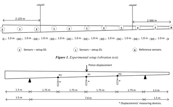
Figure 1. Experimental setup (vibration test).
Figure 2. Experimental setup (bending test).
Table 1. The nominal dimensions of the poles.
Dimensions and Materials Nominal value
Length, L [m] 10
Outer diameter at the bottom, dbot [mm] 400 Outer diameter at the top, dtop [mm] 250 Wall thickness at the bottom, tbot [mm] 62 Wall thickness at the top, ttop [mm] 52
Table 2. The nominal properties of materials of the poles.
Dimensions and Materials Nominal value Concrete grade C80/95
Prestressing strands 7/16” St 1680/1880 Number of strands, n 10
Area of the strand, APT [mm2] 70 Prestressing initial stress, b [MPa] 975
3.2. Experimental Programme
A set of experimental tests was conducted at the Bauhaus-University Weimar within the DFG research training group 1462. In the frame of this work, two types of experiments were selected. The first test is a vibration test from which system identification is achieved. The second test is a 3-point bending test, which represents both linear and non-linear behavior of the structure.
3.2.1. Vibration Test
A pole was tested using a vibration test in the free-free setup by hanging it in a horizontal position using two ropes, as shown in Figure 1 A set of twelve sensors were attached to the pole in order to measure the acceleration in both horizontal and vertical directions. Two of the sensors were fixed to the top end of the pole, and considered as reference sensors while the rest were configured in two measurement setups to increase the quantity and quality of the identified
mode shapes and natural frequencies.
Moreover, an appropriate impact hammer was used to excite the structure in three positions, horizontally and vertically for each. The process was repeated for each sensor-setup. In the first sensor-setup, the sensors were attached with an in-between distance of 2 m. Then, these sensors were moved 1 m to form the second measuring setup, as shown in Figure 1 However, more details about the setup and the results of this test can be found [18]. The natural frequencies of the first fifth mode shape in the horizontal and vertical direction were calculated using the Stochastic Subspace Identification (SSI) method through MACEC toolbox [19]. The results of the vibration test are summarized in Table 3.
Table 3. The results of the vibration test in vertical (v) and horizontal (h)
directions.
Mode shape Natural frequency [Hz]
1-h 15.56
1-v 15.59
2-h 41.17
2-v 42.67
3-h 81.09
3-v 81.72
4-h 131.58
4-v 131.69
5-h 192.68
5-v 192.43
3.2.2. 3-Point Bending Test
A displacement-based 3-point bending test was conducted to the same pole in a simply-supported setup in the horizontal position. The supports were located at 1.5 m from both ends, see Figure 2 The displacements were applied in steps at the mid-span until the pole was crushed.
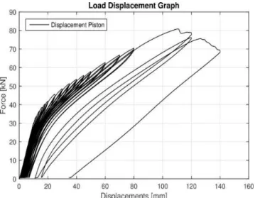
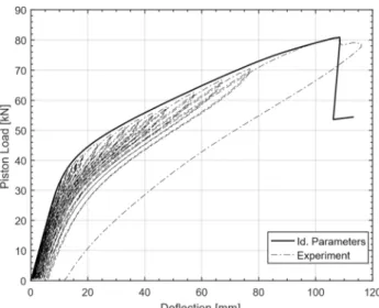
continuously in the middle and quarters of the 7 m span, i.e., at points P1, P2, and P3 shown in Figure 2 The load-displacement curve at point P1 is displayed in Figure 3, where non-linear behavior of the pole is evident. The spun-cast concrete pole behaves linearly up to a force of 25 kN, corresponding to a mid-displacement of 8 mm. Along with the cracking in the center region of the concrete pole, the stiffness of the pole decreases, leading to higher deformations for load levels above the linear range. The maximum load was 81 kN corresponding to deflection of 110 mm at the mid-span (namely, at point P1). This corresponds to the failure point of the pole, where the concrete at the most upper fiber at mid-span failed under compression.
Figure 3. Theload-displacement curve at point P1.
3.3. Finite Element Model
Finite Element Models (FEM), corresponding to each experimental test, are playing the role of the models (m) as used in Eq 1 to Eq. 4. In this aim, we build a fully-detailed FEM model to simulate each of the experimental tests.
The concrete material is simulated using volume elements, and the prestressing strands are simulated using 3D truss elements with two nodes and three degrees of freedom at each node.
The concrete constitutive model is carefully built to match both linear and nonlinear behavior of the concrete. The selected model covers the softening and hardening behavior of the concrete in tension and compression, respectively. The model has the advantage of simulating the material in the post-cracking phase, which is mainly required for simulation pole in the 3-point bending test [20].
The stress-strain curves of concrete in compression and tension are derived from the Fib Model Code 2010 [21]. The concrete in compression follows a parabolic curve until the material attains F37 corresponding to a concrete strain of 3. Then, it is followed by strain softening up till the concrete reaches a crushing strain 39 of 3.1%.
Besides, the behavior of concrete in tension is considered as linear until the mean tensile strength of concrete F347 is reached. Then, it reduces linearly to the maximum tensile
strain of the concrete.
The constitutive model of the steel follows the elastic-plastic behavior to cover the expected behavior during the 3-point bending test.
3.4. Results
The deterministic and Bayesian approaches are implemented to identify the parameters of the given structure.
The vector of parameters is built from five parameters
m = { b , F37, 3, c3, F347, d3} , where b is the initial strain
of the prestressing; F37 is the compression strength of the concrete; 3 is the concrete strain at maximum compressive stress; c3 is the concrete modulus of elasticity; F347 is the concrete tensile strength; and d3 is the concrete density. The parameters are bounded during the identification process depending on the available datasheet and the engineering prejudgment based on the values recommended by FIB Model Code 2010 [21] as shown in Table 4. These values are used to define uniform priors.
Table 4. The upper and lower binderies of the selected parameters.
Parameter Boundaries
Prestressing initial strain, b [‰] 2.7 – 3.7 Concrete compressive strength,F37 [MPa] 80 – 120 Concrete strain at maximum compressive stress, 3 [‰] 2.5 – 3.0 Concrete Modulus of Elasticity,c3[GPa] 43 – 53 Concrete tensile strength,F347 [MPa] 4.0 – 6.0 Concrete density,d3[g cm−3] 2.1 – 2.5
For the selected case study, two measurement sets are considered as observations d , such as, @ = 1, 2. The observations d of the vibration test are formed from the first ten natural frequencies of the structure. On the other hand, the load-deflection curves at mid-span and quarters of the span are considered as the observations d of the bending test.
3.4.1. Results of the Deterministic Approach
For the implementation of the deterministic approach, we assume the probability distribution of the identified parameters as a normal distribution. The parameters are estimated to 95% confidence level (? = 0.05). The results of this approach are summarized in Table 5.
Table 5. Summary of the identified parameters (deterministic approach).
Parameter Mean value Standard deviation [%]
b [‰] 3.16 2.82
F37 [MPa] 105.08 1.19
3 [‰] 2.70 0.60
c3[GPa] 48.19 3.05
F347 [MPa] 5.07 0.25
d3[g cm−3] 2.27 2.04
3.4.2. Results of the Bayesian Approach
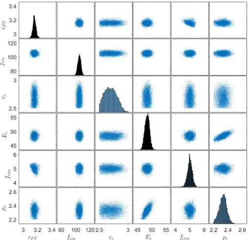
parameters are shown in the scatter plots on the same figure. The parameters c3and d3are well-correlated, as shown in the sub-plots because of the natural frequencies are proportional to the square root of the ratio between the stiffness and the mass.
Moreover, a negative correlation between F347and b can be seen. This is also understandable from the engineering point of view, as increasing the prestressing stresses raises the load corresponding to the first crack and hence decreases the inferred tensile strength of the concrete as a solution of the inverse problem. Supplementary, to get an overview of the whole applied process, the mean values, and the standard deviations are listed in Table 6.
Table 6. Summary of the identified parameters (Bayesian approach).
Parameter Mean value Standard deviation [%]
b [‰] 3.16 0.03
F37 [MPa] 105.36 1.36
3 [‰] 2.73 0.04
c3[GPa] 48.06 0.32
F347 [MPa] 5.11 0.11
d3[g cm−3] 2.32 0.04
4. Discussion
In Figure 5 we show a comparison between the results of the applied approaches. A perfect match can be recognized in the mean values of the identified parameters except for the mean values of the concrete density d3 and the concrete tensile strength F347where a small bias of 3% and 2%
respectively appeared.
However, the variance of the identified parameters differs considerably and has no specific trend, but in most cases, the variances in the Bayesian approach have higher values. From our point of view, it is expected to have such a difference between the results of deterministic and Bayesian approaches. This is because of the Markov estimator is based on the concept of the deterministic parameter identification. It may get stuck in the local minima of the cost function mainly in the case of noisy data or unidentifiable parameters. This causes the bias of the mean values comparing to Bayesian results.
Besides, the Markov estimator evaluates the uncertainty of the parameters based on local sensitivity at the optimized solution. This leads to considerable deviations of the variance values between the two approaches.
Considering the complexity and the computational efforts, we conclude that Markov estimator can be implemented mainly to have the mean values and, to some limits, an indicator of the uncertainty of the parameters. The results of Markov estimator match the results of the Bayesian approach to an acceptable tolerance, which makes Markov estimator as a fast and straightforward tool to have an approximation of the solution.
The Bayesian approach, in comparison, needs more efforts, but it can precisely draw the probability distributions of the identified parameters revealing some essential characteristics
of its distributional behavior. Besides, the Bayesian approach gives a good overview of the correlation between parameters, which leads to a better understanding of the studying problem.
In the validation step, the mean values of the identified parameters by the Bayesian approach are used as input for the FEM models. However, the results of the FEM are compared with the corresponding observations. In the case of the bending test, the results of the finite element are plotted against the hysteresis loops of the force-deflection derived from the measurements. Figures 6, 7, and 8 show the agreement between the experimental measurements of the 3-point bending test, which were measured at the mid-span and quarters, and the FEM using the identified parameter.
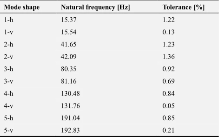
Furthermore, the first five natural frequencies in the horizontal and vertical direction, according to the test setup, are derived from the FEM model using the inferred parameters as listed in Table 7. These results show that the FEM model using the inferred parameters conforms with the experimental observations of the vibration test to an acceptable accuracy.
Table 7. Validation of the results - vibration test in vertical (v) and
horizontal (h) directions.
Mode shape Natural frequency [Hz] Tolerance [%]
1-h 15.37 1.22
1-v 15.54 0.13
2-h 41.65 1.23
2-v 42.09 1.36
3-h 80.35 0.92
3-v 81.16 0.69
4-h 130.48 0.84
4-v 131.76 0.05
5-h 191.04 0.85
5-v 192.83 0.21
Finally, we compare the inferred parameters with the conventional values of the concrete properties that are specified by the different engineering standards. In this place, we utilize the equations of the Fib Model Code 2010 [21], which specifies the concrete properties based on the compressive strength of the concrete F37. For this sake, we use the identified mean values of the F37 from Table 6. The calculated properties show that the inferred parameters are in line with the recommended values of the given model code with relatively acceptable tolerance, as shown in Table 8.
Table 8. The concrete properties based on the recommendation the Fib
Model code [21] and the identified F37.
Parameter Value The difference [%]
F37 [MPa] 105.36 ----
3 [‰] 2.90 6.20
c3[GPa] 47.10 3.10
Figure 4. The scatter plots and the histograms of the posterior distributions (Bayesian approach).
Figure 6. Validation of the results – 3-point bending test at P1.
Figure 7. Validation of the results – 3-point bending test at P2.
Figure 8. Validation of the results – 3-point bending test at P3.
5. Conclusion
In this paper, we achieved the preliminary step for
analyzing the measurements of the structural monitoring system. This system is attached to the prestressed concrete catenary poles located along the high-speed train track in Germany. Through this step, we identified the material properties of the poles to be utilized later as priors in the assessment and validation steps of the SHM system. The identification process is attained using deterministic and probabilistic approaches. In the first one, Markov Estimator is involved in quantifying the uncertainty of the identified parameters using the deterministic approach. Bayesian inference is implemented to identify the parameters in the case of the probabilistic approach. In this approach, the uncertainty of the parameters can be easily identified by calculating the statistical moments of the parameter’s distributions.
Both approaches estimated the mean values of the parameters to an acceptable tolerance. However, the Bayesian approach estimates the variances of the identified parameters in a more effective and accurate manner. Moreover, it describes the correlation between the different parameters, and then, we recommend implementing it when the parameters’ uncertainty is the main subject of interest. In the validation step, a perfect agreement is achieved when using the mean values of the inferred parameters as inputs for the numerical model and compare the results to the experimental observations.
In addition, we verify that the inferred properties of the concrete are in line with the recommended values of the Fib Model Code 2010 for the same compressive strength. The considerable deviation between the inferred parameters and the nominal ones pays our attention to the importance of the PI process before conducting any study on the existing structures. This emphasizes our argumentation at the beginning of this paper and lays the foundations for more appropriate implementation of the subsequent phases of the current case study.
Based on the recent results, we are going in the future step to trace the changes in the dynamical behavior of catenary poles on-site using Signal Processing, Operational Modal Analysis method, and Model Updating.
Acknowledgements
This work was done under the support of Deutsche Forschungsgemeinschaft (DFG) through Research Training Group 1462, which is greatly acknowledged by the authors. Another acknowledgment goes to the German Academic Exchange Service (DAAD) for supporting the main author through the scholarship Programme “Leadership for Syria.”
References
[2] Connolly, D., Kouroussis, G., Woodward, P., Costa, P. A., Verlinden, O., and Forde, M. (2014). “Field testing and analysis of high speed rail vibrations.” Soil Dynamics and Earthquake Engineering, 67, 102–118.
[3] Ampunant, P., Kemper, F., Mangerig, I., and Feldmann, M. (2014). “Train–induced aerodynamic pressure and its effect on noise protection walls.” 9th International Conference on Structural Dynamics, A. Cunha, E. Caetano, P. Ribeiro, and G. Muller, eds., EURODYN 2014, 3739–3743 (July).
[4] He, D., Gao, Q., and Zhong, W. (2018). “A numerical method based on the parametric variational principle for simulating the dynamic behavior of the pantograph-catenary system.” Shock and Vibration, 2018.
[5] Van, O. V., Massat, J.-P., and Balmes, E. (2017). “Waves, modes and properties with a major impact on dynamic pantograph-catenary interaction.” Journal of Sound and Vibration, 402, 51–69.
[6] Pombo, J. and Ambrosio, J. (2012). “Influence of pantograph suspension characteristics on the contact quality with the catenary for high speed trains.” Computers & Structures, 110, 32–42. [7] Aster, R. C., Borchers, B., and Thurber, C. H. (2013).
Parameter Estimation and Inverse Problems. Academic Press, second edition.
[8] Beck, J. V. and Arnold, K. J. (1977). Parameter Estimation in Engineering and Science. Wiley, New York.
[9] VanderPlas, J. (2014). “Frequentism and Bayesianism: A python-driven primer.” arXiv preprint arXiv: 1411.5018. [10] Idier, J. (2013). Bayesian Approach to Inverse Problems. John
Wiley & Sons.
[11] Tarantola, A. (2005). Inverse Problem Theory and Methods for Model Parameter Estimation. Society for Industrial and Applied Mathematics.
[12] Lahmer, T. and Rafajłowicz, E. (2017). “On the optimality of harmonic excitation as input signals for the characterization of
parameters in coupled piezoelectric and poroelastic problems.” Mechanical Systems and Signal Processing, 90, 399–418.
[13] Calvetti, D. and Somersalo, E. (2007). An Introduction to Bayesian Scientific Computing: Ten Lectures on Subjective Computing, Vol. 2. Springer Science & Business Media. [14] Gelman, A., Carlin, J. B., Stern, H. S., and Rubin, D. B.
(2014). Bayesian Data Analysis, Vol. 2. Chapman & Hall/CRC Boca Raton, FL, USA, third edition.
[15] Green, P. and Worden, K. (2015). “Bayesian and Markov Chain Monte Carlo Methods for Identifying Nonlinear systems in The Presence of Uncertainty.” Phil. Trans. R. Soc. A, 373(2051), 20140405.
[16] Marzouk, Y. M., Najm, H. N., and Rahn, L. A. (2007). “Stochastic Spectral Methods for Efficient Bayesian Solution of Inverse Problems.” Journal of Computational Physics, 224 (2), 560–586.
[17] Ching, J. and Chen, Y.-C. (2007). “Transitional Markov Chain Monte Carlo Methods for Bayesian Model Updating, Model Class Selection, and Model Averaging.” Journal of Engineering Mechanics, 133 (7), 816–832.
[18] Göbel, L., Mucha, F., Kavrakov, I., Abrahamczyk, L., and Kraus, M. (2018). “Einfluss realer Materialeigenschaften auf numerische Modellvorhersagen: Fallstudie Betonmast.” Bautechnik, 95 (1), 111–122.
[19] Reynders, E., Schevenels, M., and De Roeck, G. (2014). “MACEC 3.3: A MATLAB toolbox for experimental and operational modal analysis.
[20] Batikha, M. and Alkam, F. (2015). “The Effect of Mechanical Properties of Masonry on the behavior of FRP-strengthened Masonry-infilled RC Frame under Cyclic Load.” Composite Structures, 134, 513–522.