Vol 11, No 1 (2019)

(1)

International Journal of Communication Networks and Information Security (IJCNIS) Vol. 11, No. 1, April 2019

CDS-MIP: CDS-based Multiple Itineraries Planning

for mobile agents in a wireless sensor network

Rafat Ahmed Alhanani

1

_{, Jaafar Abouchabaka}

2

_,

_{Rafalia Najat}

3

1,2,3_{Department of Computer Science, IBN Tofail University, Faculty of Science, Kénitra, Morocco}

Abstract: using mobile agents in wireless sensor networks (WSNs) to aggregate sensed data has gained significant attention. Planning the optimal itinerary of the mobile agent is an essential step before the process of data gathering. Many approaches have been proposed to solve the problem of planning MAs itineraries. Those approaches assume that the planned itineraries include a large number of intermediate nodes. This assumption imposes a burden, the size of the agent increases with the increase in the visited SNs, therefore the agent consumes more energy and spends more time in its migration. None of those proposed approaches takes into account the significant role that the connected dominating nodes play as a virtual infrastructure in such wireless sensor networks WSNs. This article introduces a novel energy-efficient itinerary planning algorithmic approach based on the minimum connected dominating sets (CDSs). This approach is dedicated to the data gathering process in WSN. In our approach, instead of planning the itineraries over a large number of sensor nodes SNs, we plan the itineraries among subsets of the MCDS in each cluster. Thus, no need to move the agent in all the SNs and the intermediate nodes (if any) in each itinerary will be few. Simulation results demonstrate that our approach is more efficient than other approaches in terms of overall energy consumption and task execution time.

Keywords: Multi-Agent, Itinerary, data aggregation, Connected Dominating set, wireless sensor network.

1. Introduction

A wireless sensor network (WSN) is a network of a large number of sensor nodes where each node is equipped with limited storage, energy, processing capabilities, and deployed in sparse or dense fashion. These limitations lead to problems associated with energy consumption during the work of the sensor nodes. Sensor nodes collect information from a targeted area and transmit the complete collected data toward the central station “the Sink”. Sensor nodes can directly communicate when they are within transmission range of each other. Due to the limitation of the radio transmission range of the sensor nodes, they could not directly send the packets to a final destination, therefore they cooperatively achieve self-organized and self-routing without relying on fixed infrastructure; intermediate nodes assume the role of routers and relay the packets toward the final destination. With the lack of fixed infrastructure and the central administration, sensor nodes have to form a virtual/ temporary infrastructure to support various tasks including routing. One efficient way to form a virtual infrastructure is to use a connected dominating set (CDS). The CDS forms a virtual backbone in the network and organizes the sensor nodes into a hierarchical structure. It provides scalability, simplifies network management and guarantees network connectivity [1]. To achieve good performance, wireless network imposes strict constraints on its limited resources such as the bandwidth and energy consumption, the load on the network should be kept

as low as possible [2]. Implementing the connected dominating set CDS algorithms within WSN must be energy-efficient to prolong the lifetime of the network. Efficient algorithms should generate a small CDS size, spend low-cost overhead, and use little localized gathered information. Various CDS algorithms [3, 4, 5, 18] have been developed to address the energy conservation issue in WSNs.

Regarding the energy conservation issue in WSNs, mobile agent technique has been proposed as a middleware solution for implementing aware-energy for data aggregation schemes [6, 7, 9]. A mobile agent is an autonomous entity with the ability to move from node to another and acting on behalf of its users to complete an assigned task. It carries the processing code and its state to each visited sensor node. The resulting data after each local data processing is embedded within the agent’s state. Processed data is carried to the next sensor node, where the mobile agent resumes execution and fuses data retrieved along to its predetermined path. One of the most implementation used of the mobile agent in WSN is to aggregate data, which requires the planning and determining the nodes’ visiting order within its path, an itinerary must be scheduled. It has been proved that planning the MAs’ itinerary is an NP-hard problem [19]. The chosen itinerary largely affects the overall energy consumption and aggregation cost. Long itineraries may lead to significant energy consumption because carried data flood the agent size [10], while the overall traveling time may exceed unacceptable border for time-critical applications. In addition, inaccurate itinerary planning may drive the mobile agent to traverse unnecessary additional (intermediate) nodes during its moving among pairs of target sensor nodes (sources). The criticality of itinerary planning has motivated the design of several algorithms in order to minimize these costs. A number of studies have proposed to solve the problem of itinerary planning in sensor networks through using a Single Itinerary Planning “SIP” and using a Multi Itinerary Planning “MIP”.

In SIP, the sink node dispatches only one mobile agent to visit the whole sensor nodes in the network, whereas in MIP, the sink node dispatches several mobile agents toward different subsets of sensor nodes, they work concurrently in parallel on a target network. Each mobile agent follows its assigned itinerary “predefined subset of sensor nodes”. In contrast to SIP, MIP overcomes the drawbacks of using SIP, especially on a large WSN [11, 12]. In MIP, dispatching multi-agents decreases the packet size that is carried by each mobile agent, which has been defined as one of the SIP drawbacks.

(2)

has been addressed well in the literature by using the CDS, but without using the mobile agents. Secondly, planning efficient itineraries MIP must preserve the energy and prolong the overall life of WSNs. Thus, we propose a novel MIP algorithmic approach based on the connected dominating set CDS. Our approach determines the optimal number of mobile agents, and efficiently plans the itinerary of each agent based on an ordered list of the dominating nodes. In this way, we achieve the mentioned aspects as the planning of the itineraries is performed only among the connected dominating nodes (a virtual backbone in the WSN). Moreover, selecting the optimal number of mobile agents, which move and collect data from the selected dominating nodes (as source nodes) preserve the energy and prolong the overall life of the WSN. More details are provided in the proposed approach section. This paper is organized as follows. In the second section, we present some related works to MIP, which discuss the problem using different methods. In the third section, we explain the principle of our algorithmic approach; and how to realize minimum implementation cost by using the connected dominating set CDS as a base to construct multi itinerary planning MIP. The fourth section explains the process of our approach, and highlight our strategy through one case study. Finally, the fifth section concludes this paper.

2. State of the art on proposed MIP approaches

The mobile agent MA follows the predefined sequence of sensor nodes called the itinerary “path”. An itinerary is a route that the MA should follow during its journey. The sink node is responsible for determining this itinerary (static itinerary type). The mobile agent moves to those sensor nodes in the itinerary and performs the process of local data reduction ratio at each sensor node. Thus, eliminating the redundant of similar sensed data of closely located sensor nodes. Existing algorithms for designing the mobile agent’s itinerary are classified into single Itinerary planning SIP and multi itinerary planning MIP [12]. The first two SIP heuristics algorithms proposed in the literature are The Local Closest First (LCF) and Global Closest First (GCF) [19]. In LCF, the MA firstly moves to the nearest node to the sink, and then it searches for the closest node to its current location. In GCF, the MA uses global information related to the network (network distance matrix), it moves to the node that is nearest to the sink. In LCF algorithm, the last SNs in the MAs’ itinerary are the SNs with the longest distance to the sink, as LCF search for the next node among the remained SNs based on its current location. While the GCF algorithm produces a long itinerary and poor performance [9]. The proposed MIP algorithms include tree-based MIP, central location tree-based MIP (CL-MIP), genetic algorithm based MIP (GA-MIP), directional angle based MIP, and greatest information in the greater memory based MIP (GIGM-MIP), [12].

Mpitziopoulos et al [11] proposed a near-optimal itinerary design (NOID) algorithm. NOID algorithm calculates the number of near-optimal itineraries for the mobile agents. It adopts a method called the Esau–Williams heuristic that is based on the constrained minimum spanning tree (CMST). In each iteration, the algorithm groups the sensor nodes in the network to construct disjoined sub-trees that are connected to the sink node. Finally, it assigns an individual mobile agent to

each sub-tree starting move from the nearest sensor node to the sink node. Each mobile agent fuses the data at the nodes that belong to the assigned itinerary in the network.

Chen et al. proposed the CL-MIP algorithm [15] to determine the proper number of mobile agents and partition the network based on the density of existing nodes in different zones. The CL-MIP algorithm is an extended version of the multi-SIP algorithm. The special idea in the CL-MIP is the way that the network area has partitioned using the VCL algorithm. VCL algorithm groups the sensor nodes as following: each sensor node selects and broadcasts random impact factor, the random number in the range [0, 1), to its neighbor nodes in its transmission range. The location of the sensor node that receives the largest impact factors value from other sensor nodes will be selected as a VCL central point. Then, the source nodes within the radius of VCL assigned to the mobile agent. This process repeated to selecting a new location for the VLC sensor node, grouping the remaining nodes and assigning it to a new mobile agent. The number of determined mobile agents is large and remained sensor nodes are added to new VCL in another step at the end of the implementation.

Direction angle-based MIP algorithm (AG-MIP) is proposed for grouping all the source nodes in a particular direction zone [17, 21]. The main idea of direction-based MIP is to divide the network into zones. Based on the VCL algorithm, the AG-MIP algorithm determines two locations, the location of the VCL source node and the location of the nearest source node to the sink node. Then a direction is drawn from the VCL location toward the nearest node located in the transmission range of the sink node. Finally, all nodes around each selected central location (VCL) within this zone must be included in the same group. Each agent starts following its planned itinerary from the selected nearest node to the sink node. A particular angle gap threshold determines the boundary of each zone.

Konstantopoulos C, proposed another tree-based algorithm named second near-optimal itinerary design (SNOID). An improved version of NOID algorithm [26]. The network area is partitioning around the sink node into circular zones. The number of nodes within the radius of the sink node zone represents the number of mobile agents and the corresponding number of their itineraries. The direction of mobile agents’ itineraries starts from the first zone and extends to outer zones. The first zone includes the sink node and its neighbor nodes within its maximum transmission range. The first radius can be calculated by a.rmax, where a is an input parameter in the range [0, 1] and rmax is the maximum transmission range of any sensor node in this zone [16]. An improvement to the basic algorithm NOID has been obtained based on a tree-based itinerary design (TBID), it creates low-cost itineraries for each individual mobile agent.

Finally, an Optimal Multi-Agents Itinerary Planning (OMIP) is presented in [8], divide the network into clusters and define the cluster heads in each cluster. Starting from the cluster heads, the planning of the itineraries is realized among the source nodes using a modified version of the LCF algorithm called (MLCF).

(3)

alleviates the broadcast routing overhead by reducing the rebroadcasts (or redundant broadcasts), as the number of nodes responsible for routing is reduced to the number of nodes in the backbone. Finding the dominating set is a well-known approach, proposed for clustering the wireless ad hoc networks in various researches. All those works are implemented without using the multi-agent technique. Additionally, the connected dominating set has not used as a base for planning the itinerary of the mobile agent in the WSNs. In our earlier work [25], we analyze different techniques of constructing a connected dominating set based on the traditional marking process, the Maximal Independent Set MIS, and Multi-point Relays algorithms using the mobile agent.

3. The proposed approach

In this section, we present our CDS-based multi itineraries planning. The CDS-MIP algorithm centrally runs in the sink node SN0. It involved three main phases to realize itinerary planning. Firstly, partition the network using the K-means algorithm, this phase produces a set of clusters; then in each

introduced cluster, a minimum CDS is constructed; finally, in each cluster, we define the groups of dominating nodes that are included in the itineraries of the mobile agents, as well as determine the optimal number of mobile agents. Our model and the simple resultant of CDS-MIP is shown in Fig.1, which illustrates three clusters that introduced by the K-means algorithm, one connected dominating set CDS is built in each cluster. The node degree considers as the main criterion to select any dominating node. We assume that the dominating nodes are the source nodes. Thus, a specific number of agents are dispatched to each cluster, the agents move from the nearest dominating node to the sink node SN0, start collecting the data from the farthest dominating nodes and return to the sink node. The zone of the sink node is covered by the radius

α.Rmax [16], where Rmax denotes the maximum transmission

range and α is an input parameter in the range (0,1]. More details illustrated in the following sections.

Fig.1 simple output of CDS-MIP, three disjoined CDSs based itineraries, Red nodes are dominating nodes; Gray nodes are covered nodes.

3.1. Network Model

We model the wireless network formed by the sensor nodes SNs as an undirected graph G = (V, E), where V= {v1, v2, ... , vn} represents the set of all sensors nodes and all possible set of communication links among the sensor nodes represented by E. We assume that, each one-hop communication link (i, j) ∈ E between the sensors SNi and SNj has an equivalent energy cost that required to transfer a byte of data between these nodes; all the sensor nodes are static; have a unique identifier (ID); also, all SNs have the same amount of energy. We assume that the sources nodes are the dominating nodes. We suppose that the sink node is located at the center of the monitoring area, it has all the required information about SNs, such as location coordinates by using GPS or localization algorithms. The SNs and the sink have the same maximum

transmission range, but in terms of battery power and computational capabilities, the sink is more powerful than the other SNs.

Given a node v in G, we define the following variables that will be used:

• N1(v) is the set of one-hop adjacent nodes to the node v : N1(v)={uV/  (v, u)E}.

• N1[v] is N1(v) ∪ v.

• The degree of node v is the number of one-hop adjacent nodes uN1(v), d(v)=|N1(v)|.

• The simple , refers to the maximum degree in the graph.

3.2. Network Partitioning

Our aim by using the k-means algorithm here is to partition the network zone into k clusters. K-means algorithm is SN0

Cluster 1 Cluster 3

Cluster 2

18

17 16

15 14

13

12 10

9

8

5 4

3 2

7

6 11

(4)

commonly used and adopted in WSN for the clustering purpose [5, 14, 22, 24]; thus n sensor nodes SNi: i



[1 ,2, …..n] are partitioned in to k clusters Pj



[1 ,2, …..k] (k < n) from k centers “Cj” chosen arbitrary. K-means intends to find the positions



i, i=1...k of the centroids that minimize the distance among the sensors nodes within each cluster Pj using the equation (1). In our approach, the K-means algorithm centrally runs at the sink node; it computes the distance among n sensor nodes and all the initial centers Cj, joins each sensor node to the nearest partition Pj; therefore selecting new centroids and forming other clusters.

K-means algorithm iteratively operates to minimizing an objective function given by equation (1).

∑ ∑ 𝑑(SN,i) = min ∑ ∑ ‖SN −i‖2

𝑆𝑁∈Si 𝑘

𝑖=1 𝑆𝑁∈Si

𝑘

𝑖=1

(1)

In each iteration, it recalculates the position of the centroid in each cluster and checks the change in position from the previous one. After calculating the k new centroids, a new binding has to be done between the same set of sensors nodes and the nearest new centroid. We use the equation (2) to calculate the position of new cluster centroid:

i = (1/𝑆𝑖) ∑ 𝑆𝑁𝑗, ∀i (2)

𝑗∈Si

After K generated iterations, we may notice that the k centroids change their locations systematically until no more changes of the centroids’ positions and all sensor nodes are ranged in their partition. After the centroid positions are finalized in the clustering process, we construct each cluster Pj by including the sensor nodes that are located in the rang Rmax of the centroid Cj of each partition.

The output of this algorithm is a group P = {p1, … pk} of clusters, each cluster includes a subset of SNs, these subsets will be used in algorithm2 to construct a set of connected dominating sets, one CDS in each cluster.

3.3. Determining the MCDS in each cluster

The output of the k-means algorithm is used in the CDS-MIP algorithm as an input to construct the minimum connected dominating set MCDS in each cluster. To realize that, we select the dominating node by calculating the degree of the node; and then the Multi-Point Relay set of the node using the notation of free neighbor together with the two conditions a,b as following:

For each node s in the cluster Pj: 1. Compute the degree of the node s.

2. Add all free neighbor nodes of s, FN(s), to the MPR(s) set.

3. Add u ∈ N1(s) to MPR(s) if one of the following conditions holds:

a. If there is an uncovered node in N2(s) that is covered only by u.

b. If u covers the largest number of uncovered nodes in N2(s) that have not been covered by the current MPR(s). Use node degree to break a tie when two nodes cover the same number of uncovered nodes.

Then, to ensure selecting the minimum number of dominating nodes, we use two rules proposed by Chen and Shen in [20]. We observe that the node degree is more related to the size of the CDS instead of the node ID. Therefore, based on this observation, we replaced the ID by the degree of the node in our implementation. After computing the MPR sets of all the nodes, a node s is selected as a member in the MCDS if it is compatible with the following rules:

Rule 1: It has the largest degree than all its neighbors and it has two unconnected neighbors.

Rule 2: or it is a multipoint relay that is selected by its neighbor and has the largest degree.

CAlgorithm: generates K clusters from a set of n sensor nodes:

Input: S= {SN1, ... , SNn} ∈N (n Sensor Nodes)

1. Select a random subset Cj of S as the initial set of Cluster center;

2. While the termination criterion is not met (No change in position of any centroid) do

3. For (i=1;i≤ N; i=i+1) do

4. Using the equation (2), Attribute the closest cluster of Cj, j=1, …..k to each sensor node SNi, i=1, ….n using the Euclidean distance;

5. End For

6. Recalculate the cluster centers; 7. For (j=1; j ≤ k; j = j+1) do

8. Cluster Pj contains the set of sensor nodes SNi that are nearest to the center Cj;

9. Pj = {SNi | 𝑑(SNi, cj) = 𝑚𝑖𝑛};

10. Using the equation (3) Calculate the new position of center Cj as the mean of the points that belong to Pj; 11. EndFor

12. End While

Output: P = {p1, ... , pK} of K clusters and SNi sensor nodes in each Pj

After grouping the SNs in their clusters using the CAlgorithm, the CDS-MIP algorithm constructs one CDS in each cluster. Thus, for each node s in each cluster, the CDS-MIP computes the degree of s and the degree of its neighbor nodes N1(s) in order to specify which node of N1[s] has the maximum degree, MaxDeg(N1[s]). Computing the MaxDeg() line 7 and Multi-point Relay set of each node lines 10-11 are essential to determine if the node s is qualified to be a dominating. Two rules are used to add the node to the minimum connected dominating set (Qualified-list), lines 14-22 CDS-MIP algorithm. As proposed in [23] that these rules guarantee the shortest distances among the connected dominating nodes. The output of the CDS-MIP Algorithm is a group of minimum connected dominating sets MCDSs that will be used to plan the itineraries of MAs.

CDS-MIP Algorithm

//Constructing a set of CDSs in K clusters.

Input: set P = {p1, ... , pK} of K clusters, and Si sensor nodes in each pi.

1. Qualified-list  φ; 2. For each p∈ Pj do

// Cluster Pj contains the set of sensor nodes Si;

(5)

4. FN(s)  φ;

5. Compute the N1(s); //one-hop neighbor nodes of s 6. Compute deg(s); // the degree of s

7. Compute the MaxDeg(N1[s]); // the maximum degree of the node s and its one-hop neighbor nodes

8. Compute the N2(s); // Tow-hop neighbor nodes of s

9. Compute the FN(s); // Free Neighbor nodes of s

10. Compute the MPR(s); // Multi-point Relay 11. MPR(s)= MPR(s) ∪ FN(s);

12.End 13.End

//Add s to the minimum connected dominating set (Qualified-list) according to the following rules:

14. For (i=1, i < deg(s), i++ ) do

// Does s have two unconnected neighbors? 15. For each(m, n∈ N1(s); n≠m ) do

16. If m∈N1(n) and n∈N1(m) then s.qualified=false else Qualified-list = {Qualified-list ∪s};

17. If (deg(s) = Maxdeg(N1[s])and s.qualified=True) then Qualified-list = {Qualified-list ∪s};

18. End

19. For each(x∈ N1(s)) do

20. If (deg(x)= Maxdeg(N1[g] and s∈ MPR(x)) then Qualified-list = {Qualified-list ∪s};

21. End 22.End

23. MCDSi: {Qualified-list}; 24. SNi

min: {v ∈ MCDSi: which has the minimum distance to the Sink node and the highest remained energy };

End

Output: set of minimum connected dominating sets MCDSi that covers all the sensor nodes Si in each cluster Pj.

3.4. The optimal number of MAs and MCDS-Based Itinerary Planning

In this section, we plan the itineraries and determine the optimal number of mobile agents in each cluster. We use Dijkstra’s algorithm (minimum hop-count) to construct the shortest paths among the dominating nodes, which represent the actual communication path. A better choice is to use Dijkstra's algorithm in each dominating node since the running time of repeated Dijkstra's is better than the running time of another algorithm to finds all pairs shortest path. Implementing the Dijkstra's algorithm in a dominating node induces the shortest path tree (SPT) with several branches that are rooted at this dominating node. Since the dominating nodes are directly (one-hop) connected, few numbers of intermediate nodes have existed in the shortest path between

some dominating nodes. The idea is to divide the constructed MCDS in each cluster to subsets of CDSs. To realize that, we select one dominating node DN and construct the shortest path tree (SPT) with several branches stem from this DN, each branch extends through a specific number of dominating nodes. Thus, we group the dominating nodes in those branches based on the shortest path among them.

In order to select the appropriate DN in which the shortest path tree (SPT) will be constructed, we compute the length of the MCDS, namely the path with largest hop-count between each pair of dis-adjacent (are not adjacent) dominating nodes. This path must pass through a large number of the dominating nodes. Thus, we select the DN that is located in the middle of this path; we called this DN “D-center”.

(6)

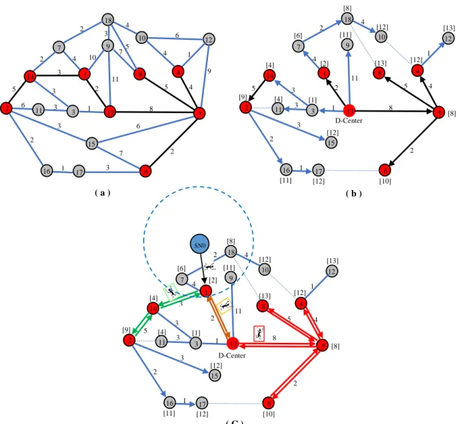
Figure 2.(a): the constructed minimum connected dominating set MCDS in a Cluster 2 in Fig.1; (b): Three branches stem from the constructed shortest path tree in the “D-Center ”dominating node 13; (c): Three mobile agents are dispatched from

the dominating node 1 (nearest dominating node to the sink) to the farthest dominating nodes {2, 8, 13}in each branch.

In our example, Fig2.(c) shows three planned itineraries. The dominating node 1 is the nearest dominating node that is located in the transmission range of the sink node. From the dominating node 1, the farthest dominating nodes in the branches of the “D-Center” node 13 are {2, 8, 13} nodes. The sink node dispatches one mobile agent to the dominating node 1; when the agent arrives, it clones itself according to the branches’ number that contain dominating nodes. Therefore, the agent at node 1 clones itself two times in order to move to the dominating nodes {2, 8, 13}. The itinerary of each agent contains arranged dominating nodes in each branch that must visit by the agent. The agent starts collecting the data from the {2, 8, 13} nodes, it uses the shortest paths information introduced by Dijkstra's algorithm to efficiently moving between each pair of dominating nodes and finally returns to the sink node.

The data collected at each dominating node are reduced only by a certain ratio f (0 < f < 1). Thus, each sensor node stores Sdata raw data, the size of data collected by the mobile agent

on the i visited sensor node can be written as iSdata = iSdata f. The total energy consumption is defined by the equation (3).

𝑇𝑜𝑡𝑎𝑙𝑐𝑜𝑠𝑡 = ∑𝑘𝑗=1𝐸𝑡 (3)

The total energy consumption in each branch of the constructed STP can be described by equation (4).

Et = ESN0_to_Ldn + ELdn_to_SN0 (4)

Where the ESN0_to_Ldn is the energy consumed by moving each mobile agent from the sink node passing through the nearest dominating node toward the farthest dominating node in each branch stems from the STP of the “D-Center” dominating node, without aggregating any data. ELdn_to_SN0 is the energy consumed by moving the mobile agent to aggregate data starting from the last dominating node toward the sink node passing through the dominating nodes belong to the branch. To compute the energy consumed ESN0_to_Ldn, equation (5) is used. Where NB-CDS is the total number of the connected

dominating nodes in each branch. ESN0_to_Ldn = (Scode+Sstate).NB-CDS (5) 2 3 D-Center [4] 2 3 6 1 2 1

3 ₁ ₈

5 4 1 4 11 2 4 3 2 5 18 17 16 15 14 13 12 10 9 8 5 4 3 2 7 1 6 11 [8] [10] [12] [11] [12] [13] [12] [8] [6] [2] [1] [9] [12] [11] [13] [4] 6 2 3 7 6 3 6 1 2 1

3 1 8

5 4 9 1 4 6 4 5 7 11 10 2 3 4 3 2 2 5 3 18 17 16 15 14 13 12 10 9 8 5 4 3 2 7 1 6 11 D-Center [4] 2 3 6 1 2 1 1 8 5 4 1 4 11 2 4 3 5 18 17 16 15 14 13 12 10 9 8 5 4 3 2 7 1 6

11 _[8]

[10] [12] [11] [12] [13] [12] [8] [6] [2] [1] [9] [12] [11] [13] [4] 3 SN0

( C )

(7)

To compute the energy consumed ELdn_to_SN0 for each CDS based itinerary in each branch to aggregate the data the equation (6) is used.

ELdn_to_SN0= ∑ ((𝑖𝑓𝑆𝑑𝑎𝑡𝑎+ 𝑆𝑐𝑜𝑑𝑒+ 𝑆𝑠𝑡𝑎𝑡𝑒) ∙ (𝑒𝑡𝑥

1

|𝑁B−CDS|

+ 𝑒𝑟𝑥)) (6)

Where etx is the energy transmission and erx the energy receiving cost respectively associated with transferring and receiving one byte between pair of directly connected dominating nodes. Sstate is the mobile agent’s initial size; Scode is the execution code size that carried by the mobile agent.

3.5. Fault tolerance based on selecting alternative CDS-based itinerary

Unfortunately, nodes in the dominating set consume more energy in handling various bypass traffic than nodes outside the set. We propose a method of calculating power-aware connected dominating set based on a dynamic selection process, given the preference to a node with a higher energy level. Because the topology of the network changes over time, as some sensor nodes drain their energy and become deactivated, the connected dominating set also needs to be updated periodically from time to time, the mobile agent verifies that during its move among the predefined CDS-based itinerary. Those connected dominating sets are expected to be changed after the mobile agent visits them based on their remained energy. Thus, the mobile agents inform the sink, which in turn periodically reconstructs new MCDS in each cluster. This change preserves the energy balance among the selected connected dominating nodes. In order to prolong the network life, alternative itineraries are taken into consideration; the itineraries derived by CDS-MIP algorithm must be modified over consecutive data aggregation rounds and before any dominating node fails. Thus, different dominating nodes will be consecutively replaced to share the amount of consumed energy especially those dominating nodes being closer to the sink node, since these nodes suffer from extra data forwarding burden.

4. Experimental results and Simulation settings

We have implemented the proposed CDS-MIP algorithm using Castalia [27] simulation platform. We compared our algorithm with two Minimum Spanning Tree-based MIP algorithms NOID [26] and BST [13]. The size of the simulated zone has been set to 500 × 500 m2. All the nodes randomly deployed in the network zone, varied from 100 to 600 nodes and the sink node is located at the center of the zone. The parameters for the simulation (shown in Table 1) are considered to evaluate the performance of the proposed algorithm in sparse and density network.

We consider the following performance metrics:

− Overall energy consumption is the consumed energy by all sensor nodes and the mobile agents to visiting and aggregating data from the minimum connected dominating nodes MCDS.

− The number of mobile agents MAs (equivalent to the number of itineraries) that will be dispatched to aggregate

data from the minimum connected dominating nodes MCDS.

− Execution time: it is the required time for all MAs to execute one round of data aggregation.

Table 1: Simulation Parameters.

Parameters Value

Simulated terrain 500 × 500 m2

Agent code size 1024 bit

Agent accessing delay 10 ms

Size of collected data at dominating node 2048 bits

Aggregation ratio 0.9

The initial energy of nodes 0.5J Energy consumed for Mobile agent execution (data aggregation)

5 nJ Energy consumed for sensing 0.02 mJ

Network transfer rate 250 Kbps

Raw data reduction ratio (r) 0.8 Size of processing code (Scode) 2MB Topology configuration mode Randomized Fig.3 shows the overall energy consumption, comparing our approach to other approaches, CDS-based approach consumes less energy with the increase in the size of the network. In the case of 100-200 nodes, the network is sparse and the average number of constructed CDS in each cluster is relatively high; the CDS-MIP outperforms other approaches, as the dominating nodes are grouped (sub-sets of CDS) in the branches of the Shortest Path Tree; therefore, the itineraries are planned based on the limited number of connected dominating nodes.

Fig.3 Overall energy consumed of our CDS based approach comparing to other approaches.

Fig.4 number of constructed CDS.

A shown in Fig.4, the number of connected dominating nodes is a perfect percentage rate to the total number of the network

100 10000

100 200 300 400 500 600

OV

E

R

A

L

E

NE

R

GY

C

ON

S

UPT

ION

NUMBER OF SENSOR

NOID BST CDS-MIP

15 20 25 30 35 40 45

100 200 300 400 500 600

C

DS

S

iz

e

in

a

v

er

age

(8)

nodes. Thus, the length of itineraries planned by CDS-MIP algorithm are short as well. While other approaches plan the itineraries based on the minimum spanning tree, which spreads over all the nodes in the network or a portion of the network; therefore, the agent will be obligated to traverse long itineraries with additional intermediate nodes.

In the case of 300-600 nodes, in spite of the relative increase on the selected dominating nodes in each cluster (dense network); the performance of our approach is still good. As one dominating node can cover a big number of adjacent nodes and the planning of the itinerary is based on a subset of dominating nodes with few numbers of intermediate nodes (if any). Thus, the agent will perform a few numbers of moves. While in MST based approaches, the number of intermediate nodes in the spanning tree is increased with the increase in the deployed nodes; thus, the agent will perform big numbers of moves.

In order to start the data collection task, MAs in BST and NOID approaches typically moves via the intermediate nodes located along their itineraries. MA follows a path including several intermediate nodes, no data is collected at these nodes, energy is consumed to receive and retransmit the MA with its aggregated data from the source nodes; therefore, additional hops will be performed that increase the overall energy consumption, implementation time and affect the performance rate. Consequently, MA carries aggregated data from their assigned nodes while moving towards the sink with additional cost. NOID consumes more energy than BST mainly because it commonly derives long itineraries, hence, reducing the number of resulting itineraries.

It is observed that the rate change of the energy consumption in CDS-MIP algorithm is significantly low, because the maximum payload of the agent is relatively fixed in the CDS-MIP, and the intermediate nodes in each itinerary are few. However, for minimum spanning tree based approaches, there is no restriction on the included nodes (intermediate nodes) in the itinerary, therefore the payload size of the agent increases, which is resulting in more energy consumption.

Fig.5 illustrates the execution time required for traveling the mobile agents to visit all CDS for delivering the collected data to the sink. It compares our proposed approach CDS-MIP to NOID and BST approaches in term of execution time. It is obvious that the execution time is directly proportional with the joined nodes in each itinerary or with an increase in the number of the dispatched agent. The service time is determined by the time elapsed when the first mobile agent is sent to the network until the last mobile agent returns to the sink.

Fig.5 the time required for traveling the mobile agents to visit all source nodes.

Our CDS-MIP algorithm maintains stable execution time as the network size increases. Each itinerary contains a specific subset of connected dominating nodes, and the intermediate nodes (if any) exist only when the agent moves from the nearest dominating node that is located in the transmission range of the sink to the farthest dominating node in each branch. While in NOID and BST approaches undoubtedly have longer execution times that are produced, as MAs need more time to travel along their itineraries that contain numerous intermediate nodes. The results indicate that CDS-MIP outperforms other approaches in term of execution time and energy consumed due to construct efficient itineraries based on sub-sets of CDS.

Finally, Fig.6 shows the number of itineraries (which is the equivalent to the number of dispatched MAs) in NOID, BST approaches and our CDS-MIP approach. NOID has the highest number of dispatched MAs, followed by BST while our CDS-MIP approach manages the optimal number of the dispatched MAs.

Fig.6 Total number of itinerariesintroduced by our CDS-MIP approach comparing to other approaches.

As shown in Fig.7, although NOID generates the largest number of itineraries, those itineraries have the higher number of intermediate nodes, which cause a high increase in the execution time and the agents performed large numbers of transfers. The mobile agents require multiple hops to reach the first source node and return from the last one. While our approach generates the optimal number of the itineraries that are corresponding to a specific number of dominating nodes subsets in each branch.

Fig.7 Total number of transfers performed by MAs. 3

30 300

1 0 0 2 0 0 3 0 0 4 0 0 5 0 0 6 0 0

EXE

CUT

IO

N

T

IME

(

SE

C)

NUMBER OF SENSORS BST NOID CDS-MIP

1 10 100

100 200 300 400 500 600

NU

M

B

E

R

OF

I

T

INE

R

A

R

IE

S

NUMBER OF SENSORS

BST NOID CDS-MIP

10 100 1000

1 0 0 2 0 0 3 0 0 4 0 0 5 0 0 6 0 0

TO

TA

L

N

UM

B

ER

O

F M

A

T

R

A

N

SF

ER

S

(9)

5. Conclusion

In this work, we proposed a new approach for planning and constructing efficient multi itineraries MIP based on the connected dominating sets CDS-MIP. We adapt the k-means algorithm in order to partition the network and distribute the sensor nodes in equivalent clusters, k-means algorithm is used effectively to draw the boundaries among the clusters and to group the nodes according to their distances toward each cluster heads called centroids. Thus, we construct a minimum connected dominating set MCDS in which all SNs in this region efficiently communicate due to this virtual infrastructure. This MCDS is a backbone by which one mobile agent can efficiently aggregate the data in this region. Since each non-dominating sensor node directly connects to at least one connected dominating node (one hop away), the agent aggregates the data of the dominating node and the sensed data of the adjacent nodes that are covered by the dominating node. In order to achieve balanced CDS based itineraries, we introduce a method of constructing subsets of connected dominating nodes from the main MCDS in each cluster. To realize that, we specified the length of the MCDS which is the maximum hop counts number between each pair of dis-connected dominating nodes; the path must include the maximum number of dominating nodes. We construct the shortest path tree SPT in the dominating node (called D-Center) that is located at the center of this path. Thus, branches of SPT are stemming from the D-Center, and each branch contains a subset of dominating nodes. Finally, planning of each itinerary will start from one dominating node (sensor node) in each cluster, which is located at the transmission range of the sink node (nearest dominating node to the sink). One mobile agent will be dispatched to each branch of the SPT; it uses the shortest path information to move between the nearest dominating node and the farthest dominating node in each branch. The agent then starts collecting the data from the farthest node passing through the dominating nodes in each branch toward the sink node. Simulation results show that our CDS-MIP approach outperforms other approaches in term of execution time and energy consumed due to constructing efficient itineraries based on sub-sets of CDS.

References

[1]. A. Aziz, Y. A. Sekercioglu, "A distributed energy aware connected dominating set technique for wireless sensor networks," Proceedings of the 4th International Conference on Intelligent and Advanced Systems (ICIAS 2012), Kuala Lumpur, Malaysia, Vol. 1, pp. 241-246, 2012.

[2]. H. Beigy, M.R. Meybodi, “Utilizing distributed learning automata to solve stochastic shortest path problems,” International Journal of Uncertainty, Fuzziness, and Knowledge-Based Systems Vol. 14, No. 05, pp. 591-615, 2006.

[3]. D. Kim, Y. Wu, Y. Li, F. Zou, and D. Z. Du, “Constructing minimum connected dominating sets with bounded diameters in wireless networks,” IEEE Transactions on Parallel and Distributed Systems, Vol. 20, No. 2, pp. 147– 157, 2009.

[4]. Z. Yuanyuan, X. Jia, and H. Yanxiang, “Energy efficient distributed connected dominating sets construction in

wireless sensor networks,” Proceedings of the 2006 International Conference on Wireless Communications and Mobile Computing, IWCMC 2006, Vancouver, British Columbia, Canada, p. 802, July 3-6, 2006.

[5]. W.Gicheol and C.Gihwan, “Securing Cluster Formation and Cluster Head Elections in Wireless Sensor Networks,” International Journal of Communication Networks and Information Security (IJCNIS), Vol. 6, No. 1, pp.71-88, 2014.

[6]. Dong, M., Ota, K., Yang, L. T., Chang, S., Zhu, H., & Zhou, Z, “Mobile agent-based energy-aware and user-centric data collection in wireless sensor networks,” Computer Networks, Vol. 74, pp.58–70, 2014.

[7]. Mpitziopoulos, Aristides, Damianos Gavalas, Charalampos Konstantopoulos and Grammati E. Pantziou “Mobile agent middleware for autonomic data fusion in wireless sensor networks,” Autonomic Computing and Networking, Chapter 3 in book, pp. 57-81, 2009.

[8].Rais Amine, Bouragba Khalid & Ouzzif Mohamed, “Determination of Itinerary Planning for Multiple Agents in Wireless Sensor Networks,” International Journal of Communication Networks and Information Security (IJCNIS), Vol. 10, No. 1, April 2018.

[9]. Gavalas, D, Venetis, IE, Konstantopoulos, C, “Energy-efficient multiple itinerary planning for mobile agents-based data aggregation in WSNs,” Telecommunication System, Vol. 63, pp. 531–545, 2016.

[10].Paul, T. & Stanley, K. G., “Data collection from wireless sensor networks using a hybrid mobile agent-based approach,” Proceedings of the 2014 IEEE 39th conference on local computer networks LCN’2014, pp. 288–295, 2014.

[11].Mpitziopoulos A, Gavalas D, Konstantopoulos C, et al, “Deriving efficient mobile agent routes in wireless sensor networks with NOID algorithm,” In: IEEE 18th international symposium on personal, indoor and mobile radio communications PIMRC2007, Athen Greece, pp. 1– 5, September 2007.

[12].Wang X, ChenM, Kwon T, et al, “Multiple mobile agents’ itinerary planning in wireless sensor networks: survey and evaluation,” IET Communication, Vol. 5, No.12, pp. 1769–1776, 2011.

[13].Chen, M., Cai, W., Gonza´lez, S., & Leung, V. C. M, “Balanced itinerary planning for multiple mobile agents in wireless sensor networks,” Proceedings of the Second International Conference in Ad Hoc Networks (ADHOCNETS’2010), Victoria, BC, Canada, pp. 416– 428, August 18-20, 2010.

[14]. A. Aloui, O. Kazar, L. Kahloul, S. Servigne, ” A new Itinerary planning approach among multiple mobile agents in wireless sensor networks (WSN) to reduce energy consumption,” International Journal of Communication Networks and Information Security (IJCNIS), Vol.7, No.2, 2015.

[15]. Chen M, Gonzalez S, Zhang Y, et al, “Multi-agent itinerary planning for wireless sensor networks,” 6th International ICST Conference on Heterogeneous Networking for Quality, Reliability, Security and Robustness, QShine 2009 and 3rd International Workshop on Advanced Architectures and Algorithms for Internet Delivery and Applications, AAA-IDEA 2009, Las Palmas, Gran Canaria, Spain, pp. 584–597. 2009.

(10)

[17].Cai W, Chen M, Wang X, et al, “Angle gap (AG) based grouping algorithm for multi-mobile agents itinerary planning in wireless sensor networks,” Proceedings of Symposium of the Korean Institute of communications and Information Sciences, Seoul, Republic of Korea, Vol. 11, pp. 305–306, 2009.

[18].B. Han, W. Jia, “Clustering wireless ad hoc networks with weakly connected dominating set,” Journal of Parallel and Distributed Computing, Vol. 67, pp.727–737, 2007.

[19].G Chen, S Wu, J Zhou, AKH Tung, “Automatic itinerary planning for traveling services,” IEEE Transactions on Knowledge and Data Engineering , Vol. 26, No.3, pp. 514-27, 2014.

[20].X. Chen and J. Shen, “Reducing connected dominating set size with multipoint relays in ad hoc wireless networks,” Proceedings of the 7th International Symposium on Parallel Architectures, Algorithms and Networks, Hong Kong, China, pp. 539 - 543, May 2004.

[21].M. Chen, S. Gonzalez, V. Leung, "Directional source grouping for multi-agent itinerary planning in wireless sensor networks," 2010 International Conference on Information and Communication Technology Convergence (ICTC), Jeju, South Korea, pp. 207-212, 2010.

[22].A. Likas, N. Vlassis, J. Verbeek, " The global k -means clustering algorithm," Pattern Recognition ., Vol. 36, No. 2, pp. 451-461, 2003.

[23].L. Ding, X. Gao, W. Wu, W. Lee, X. Zhu, D.-Z. Du, “An exact algorithm for minimum CDS with shortest path constraint in wireless networks,” Optimization Letters, Vol. 5, No. 2, pp. 297–306, 2011.

[24].T. Kanungo, D. M. Mount, N. S. Netanyahu, C. D. Piatko, R. Silverman and A. Y. Wu, "An efficient k-means clustering algorithm: analysis and implementation," in IEEE Transactions on Pattern Analysis and Machine Intelligence, Vol. 24, No. 7, pp. 881-892, Jul 2002.

[25].R Alhanani, Jaafar Abouchabaka, Rafalia Najat, “New approach to construct a minimum connected dominating set using Mobile Agent,” 3th International Conference on Big Data, Cloud and Applications, (BDCA’18), Morocco, pp. 120-132, 2018.