Hybrid Bees Approach Based on Improved Search Sites Selection by
Firefly Algorithm for Solving Complex Continuous Functions
Mohamed Amine Nemmich and Fatima Debbat
Department of Computer Science, University Mustapha Stambouli of Mascara, Mascara, Algeria E-mail: [email protected], [email protected]
Mohamed Slimane
Université de Tours, Laboratoire d’Informatique Fondamentale et Appliquée de Tours (LIFAT), Tours, France E-mail: [email protected]
Keywords: optimization, bees algorithm, firefly algorithm, memory scheme, adaptive neighborhood search, swarm intelligence, bio-Inspired computation
Received: July 25, 2018
The Bees Algorithm (BA) is a recent population-based optimization algorithm, which tries to imitate the natural behavior of honey bees in food foraging. This meta-heuristic is widely used in various engineering fields. However, it suffers from certain limitations. This paper focuses on improvements to the BA in order to improve its overall performance. The proposed enhancements were applied alone or in pair to develop enhanced versions of the BA. Three improved variants of BA were presented: BAMS-AN, HBAFA and HFBA. The new BAMS-AN includes memory scheme in order to avoid revisiting previously visited sites and an adaptive neighborhood search procedure to escape from local optima during the local search process. HBAFA introduces the Firefly Algorithm (FA) in local search of BA to update the positions of recruited bees, thus increasing exploitation in each selected site. The third improved BA, i.e. HFBA, employs FA to initialize the population of bees in the BA for a best exploration and to start the search from more promising regions of the search space. The proposed enhancements to the BA have been tested using several continuous benchmark functions and the results have been compared to those achieved by the standard BA and other optimization techniques. The experimental results indicate that the improved variants of BA outperform the standard BA and other algorithms on most of the benchmark functions. The enhanced BAMS-AN performs particularly better than others improved BAs in terms of solution quality and convergence speed.
Povzetek: Za reševanje kompleksnih zveznih funkcij so razvili nov pristop na osnovi hibridnega čebeljega algoritma (BA) in algoritma Firefly.
1
Introduction
Metaheuristic algorithms generally mimic the more successful behaviors in nature. These methods present best tools in reaching the optimal or near optimal solutions for complex engineering optimization problems [1].
As a branchof metaheuristic methods, swarm intelligence (SI) is the collective behavior of populated, self-organized and decentralized systems. It concentrates specifically on insects or animals behavior in order to develop different metaheuristics that can imitate the capabilities of these agents in solving their problems like nest building, mating and foraging. These interactions have been effectively appropriated to solve large and complex optimization problems [2]. For instance, the behaviors of social insects, such as ants and honey bees, can be patterned by the Ant Colony Optimization (ACO) [3] and Artificial Bee Colony (ABC) [4] algorithms. These methods are generally utilized to describe effective food search behavior through self-organization of the swarm.
In SI, honey bees are one of the most well studied social insects. Furthermore, it is in a growing tendency in the literature for the past few years and it will continue. Many intelligent popular search algorithms are developed such as Honey Bee Optimization (HBO), Beehive (BH), Honeybees Mating Optimization (HBMO), Bee Colony Optimization (BCO), Artificial Bee Colony (ABC) and the Bees Algorithm (BA) [5].
The Bees Algorithm (BA) is one of optimization technique that imitates the foraging behavior of honeybee in nature to solve optimization problems [6]. The main advantage of Bees Algorithm is has power and equilibrate in local search (exploitation) and global random search, (exploration), where both are completely decoupled, and can be clearly varied through the learning parameters [7]. It is very efficient in finding optimal solutions and overcoming the problem of local optima, easy to apply, and available for hybridization combination with other methods [5].
optimization [8], production scheduling [9], numerical functions optimization [5, 6, 7, 10], solving timetabling problems [11], control system tuning [12], protein conformation search [13], test form construction [14], Placements of FACTS devices [15], pattern recognition [16], robotic swarm coordination [17], data mining [18, 19, 20], chemical process [21], mechanical design [22], wood defect classification [23], Printed Circuit Board (PCB) assembly optimization [24], image analysis [25], and many other applications [26].
The BA has attracted attention of many researchers in different fields since it has been proved to be efficient and robust optimization tool. It can be split up into four components: parameter tuning, initialization of population, exploitative neighborhood or local search (intensification) and exploratory global search (diversification) [26]. However, despite different successful applications of the BA, the algorithm has some limitations and weaknesses. The algorithm efficiency is much influenced by initialization of the different parameters that need to be tuned. Additionally, the BA suffers from slow convergence caused by many repeated iterations in local search [5].
Many different investigations have been made to improve BA performance. Certain of these studies focus on the parameter tuning and setting component [27, 28]. Others developed different concepts and techniques for the local search neighborhood stage [5, 7], or global search stage [9] or for both the local and global stage [29]. Nonetheless, limited interest has been given to the improvement of the initialization stage.
In order to deal with some weaknesses of BA, this paper considers different improvements based on other strategies and procedures. Hybridization of different techniques may improve the solutions quality and enhance the efficiency of the algorithms.
The present work is an extension of the methods presented in [30]. The Firefly Algorithm (FA), which is swarm intelligence metaheuristic for optimization problems that based upon behavior and motion of fireflies [31], is applied to initialize the bee population of Basic BA for a best exploration of research space and start the search from more promising locations. FA is also introduced in the local search part of Basic BA in order to increase exploitation in each research zone. As a result, two BA variants called the Hybrid Firefly Bee Algorithm (HFBA) and Hybrid Bee Firefly Algorithm (HBAFA), respectively.
We also investigate the behavior of local search and global search of the BA by introducing two strategies: memory scheme (local and global memories) to overcome repetition and unnecessarily spinning inside the same neighborhood and avoid revisiting previously visited sites, and adaptive neighborhood search procedure to jump from the sites of similar fitness values, thus improving the convergence speed of the BA to the optimal solution. This improved variant of BA is called, Bees Algorithm with Memory Scheme and Adaptive Neighborhood (BAMS-AN).
The rest of this article is organized as follows. Section 2 provides a description of Basic BA, FA and
three improved variants of BA with different strategies. Section 3 presents and discusses the computational simulations and results obtained on benchmark instances, while Section 4 presents our conclusions and highlights some suggestions and future research directions.
2
Materials and methods
2.1
The standard bees algorithm
The Bees Algorithm (BA) is a bee swarm-based metaheuristic algorithm, which is derived from the food foraging behavior of honey bees in nature. It was originally proposed by Pham et al. [6].
The BA starts out by initializing the population of scouts randomly on the space of search. Then the fitness of the points (i.e. solutions) inspected by the scouts is evaluated. The scouts with the highest fitness are selected for neighborhood search (i.e. local search) as “selected bees” [6]. To avoid duplication, a neighborhood called a “flower patch” is created around every best solution; furthermore the forager bees are recruited and affected randomly within the neighborhoods. If one of the recruited bees lands on a patch of higher fitness than the scout, that recruited bee turns into the new scout and participates in the waggle dance in the next generation. This step is called local search or exploitation [7]. Finally, the remaining of the colony bees (i.e. population) is assigned around the space of search scouting in a random manner for new possible solutions. This activity is called global search (i.e. exploration). In order to establish the exploitation areas, these solutions with those of the new scouts are calculated with a number of better solutions being reserved for the succeeding learning cycle of the BA. This procedure is repeated in cycles until it is necessary to converge to the optimal global solution [5].
The Bees Algorithm detects the most promising solutions, and explores in selective manner their neighborhoods to find the global minimum of the objective function. When the best solutions are selected, the BA in its basic version makes a good balance between a local (or exploitative) search and a global (or exploratory) search. The both develop random search [7]. The pseudo-code of the Standard Bees Algorithm is given below in Figure 1.
A certain number of parameters are required for the BA, called: number of the scout bees or sites (n), (m) sites selected for local search among n sites, (e<m) elite sites chosen from the m selected site for a more intense neighborhood search, (nre) recruited bees for the elite sites, (nrb<nre) bees recruited for neighborhood search around other m-e best sites, initial size of all selected patch (ngh) around each scout for neighborhood search (i.e. flower patch), stopping criterion for the algorithm to terminate and number of iterations [5].
From the control settings of algorithm, the bees’ population size p can be determined as below:
(
m
e
)
nrb
nre
e
ns
where; ns is (n – m) remaining bees.
For random scouting in the initialization phase as well as for the unselected bees, the following equation is adopted:
(
max min)
min
rand
*
x
x
x
x
rand=
+
−
(1)where; rand is a random vector element between 0 to 1, xmax, xmin are the upper and lower bound to the solution vector, respectively.
Two additional steps are called when neighborhood search does not improve any fitness enhancement in a neighborhood: the neighborhood shrinking and the site abandonment. The primary objective is to enhance the computation performance and the search accuracy. This implementation is called the Standard Bees Algorithm (Standard-BA) [7].
2.1.1
Neighborhood shrinking strategy
A large value is defined for the initial size of the neighborhoods. For each ai of a = {a1, …,an} is set as follows:
( )
( ) (
i i)
i
t
ngh
t
a
=
max
−
min
( )
0
=
1
.
0
ngh
(2)where t represents the t-th iteration of the BA main loop. The initial size of flower patches is on a wide area to promote the exploration of the search space. Whilst the local search procedure gives better fitness, the size of patches is maintained unchanged, and is then gradually reduced to yield the search more exploited round the local optimal [7]. The ultimate objective of the neighborhood shrinking approach is to make the search progressively concentrated in the proximity of the local peak of fitness. The updating formula is given as follows:
(
t
)
ngh
( )
t
ngh
+
1
=
0
.
8
(3)A new variant of BA can be obtained by applying the shrinking procedure over Basic BA. This implementation is named the Shrinking-based BA [26]. It can be deducted from the first paper of Pham et al. [6].
2.1.2
Site abandonment strategy
To enhance the efficiency of the local search, the site abandonment procedure is introduced, in which there is no more enhancement of the fitness value of the fittest bee after a predetermined number (stlim) of successive
stagnation cycles. If the abandoned site corresponds to the fitness best value, the location of the peak is registered. If no other flower patch will generate a better value of fitness in the rest of the search, the better registered fitness position is taken as the final solution [7].
To sum up, in the literature review of Bees Algorithm, three important implementations could be discovered, which are Basic-BA, Shrinking-based-BA, and Standard-BA.
Bees Algorithm (BA)
Initialize population with random solutions by sending (n) scout bees. Iterate until a stopping criterion is met
1. Evaluate the fitness of the population. 2. Sort the solutions according to their fitness. // Waggle dance
3. Select the highest-ranking m solutions (i.e. sites or patches) for neighborhood search. 4. Determine the patch of each selected site with an initial size of (nghinit).
5. Recruit nr = nre foragers to each of the e≤m top-ranking elite solutions. 6. Recruit nr = nrb≤nre foragers to each of the remaining m – e selected solutions. // Local search
7. For each of the m selected solutions
a. Create nr new solutions by perturbing the selected solution randomly or otherwise and evaluate their fitness. b. Retain the best solution amongst the selected and new solutions.
// Neighborhood Shrinking Strategy
c. Adjust the neighborhood of the retained solution (i.e. Shrink patches whose neighborhood has achieved no improvement by a shrinking factor (sf)).
// Site Abandonment Strategy
d. Abandon sites where no progress has been made for a number (stlim) of consecutive iterations and re-initialize them (Save the location of the abandoned site if it represents the current best solution).
// Global search
8. Assign the remaining bees (n - m) to search randomly and evaluate their fitness. 9. Form new population (m solutions from local search, n – m from global search)
2.2
The standard firefly algorithm
Firefly Algorithm (FA) is a recent biologically-inspired algorithm originally introduced by [31]. FA imitates the communication behavior of tropical fireflies and the idealized flashing features of fireflies [31].
The primary strengths of FA are namely exploitation and exploration. In addition, the proposal time of this algorithm is relatively short, the parameters needing to be adjusted are quite few due to its simple structure and less complexity without requiring complex evolutionary operations; and the optimizing search ability is also relatively good [32].
FA has been successfully applied to solve different optimization problems such as software testing [33], dynamic multidimensional knapsack problems [34], combinatorial problem [35], mobile robotics [36], network route selection [37], linear antenna array failure correction [38], optimized gray-scale image watermarking [39], automatic control system optimization [40, 41], price budget [42], multi-objective economic emission dispatch solution [43], and so on. Generally, it can get the optimal solution with its exploitation [44].
According to [32], two important things need to be defined in FA: the change of the attractiveness (β) and the formulation of the light intensity or brightness (I).
The strength of attraction is proportional to the intensity of the brighter firefly and the distance between the two fireflies, so the brightness reduces with the distance from its source and the media will absorb the light. The light intensity of a firefly is given according to the value of the objective function. For simplicity, different features of fireflies are idealized into diverse rules detailed in [32]. The descriptive pseudo code of the FA is given in Figure 2.
The attractiveness β between two fireflies can be determined by the following equation:
(
2)
0
exp
*
r
=
−
(4)where; β0 is the attractiveness at r = 0, r is the distance of two fireflies and γ is the light absorption coefficient. γ is the most crucial parameter in FA method, it performs a very important role in determining the convergence speed and how FA behaves. Hence, nearly all the applications it differs from 0.1 to 10 [45].
The distance among any two fireflies i and j at xi and xj, respectively, calculated by the Euclidean or Cartesian distance formulation as follows:
(
)
=
−
=
−
=
dk
k j k i j
i
ij
x
x
x
x
r
1
2 ,
, (5)
Firefly i is attracted to another more attractive (brighter) firefly j and its movement is calculated by equation (7) [31]. In this equation the second part is the attraction, whilst the third is randomization with the control parameter α ∈ [0, 1], and εi is a vector of random numbers being generated from different distributions such as uniform distribution, Gaussian distribution and Lévy flight. The most basic form is εi could be changed by (rand − ½) where rand is a random real number
between interval [0 1] [32]. It is interesting that (7) is a random-walk partial to the brighter fireflies. If β0 = 0, it turns into a simple random walk. Furthermore, the randomization term can easily be prolonged to different distributions such as Lévy flights [31].
(
)
ti t j t i r t
i t
i
x
e
x
x
x
+=
+
−ij2−
+
0 1
(6)
2.3
The improved bees algorithms
In this subsection, three improved variants of BA are presented: Bees Algorithm with Memory Scheme and Adaptive Neighborhood (BAMS-AN), Hybrid Firefly-Bee Algorithm (HFBA) and Hybrid Firefly-Bee Firefly Algorithm (HBAFA).
2.3.1
Improved bees algorithm with memory
scheme and adaptive neighborhood
In this improved variant, two modifications of BA are introduced. The first one is to improve the BA in more efficient and natural manner with memory integration (local and global memories) to avoid revisiting previously visited sites and overcome repetition and unnecessarily spinning inside the same neighborhood. Thus, the search in the BA can prevent searching within infertile areas and can jump from potential local optimums. The second modification is to deploy an adaptive neighborhood search procedure to escape from local optima during the local search process.
The memory is part of the honey bees’ nature, but was not included in basic BA. The strategy is to force the bees to stay away from the neighborhoods studied and experienced with no beneficial results. This will enforce the bees to visit different solutions for investigation. This needs the integration of a memory mechanism into the bees to allow them to respect the experiences and not waste their energy and time. This type of memory will be Firefly Algorithm (FA)
Define the objective function of f(x), where
x=(x1,...,xd)T
Generate initial population of fireflies xi (i = 1, 2,..., n) randomly.
Determine the light intensity of Ii at xi via f(xi) Define α, β and γ
While (t <MaxIterFA)
For i = 1 :n (all n fireflies)
For j = 1 : n (all n fireflies)
If (Ii <Ij ), Move firefly i towards j by using equation (7); end if
Vary attractiveness with distance
r via exp[− γr]
Evaluate new solutions and update light intensity
Endfor j Endfor i
Rank the fireflies according to light intensity and find the current global best
End while
Post-process results and visualization
integrated to the scout and the follower bees where these bees could employ information and details about previously visited sites (i.e. positions and finesses). Different structures of arrays are used to save and handle the memory of each bee (scout and follower). The memory contains the information obtained during direct communication with the environment that used to decide the way of patch visiting based on a waggle dance or depend on it. This information is very important and affects the way forager bees (both scout and follower bees) choose the patch to visit and whether it will be based on a waggle dance or not (i.e., choosing a familiar food source). Foragers depend on their own memories to discover particular locations during the visit of food patches repeatedly [16, 19].
The memorized experiences are continuously updated and utilized to lead the further foraging of the bees, contributing to a more effective search procedure than basic BA.
The pseudo-code below shows the procedures added. It is included in the local neighborhood search for follower bees and in the global search for scout bees. This procedure decides if the new position (in different dimensions) of any bee is close to its previous one recorded in its memory.
where r is the radius, xd
max and xdmin are the upper and the lower bound to the solution vector respectively, itmax is the maximum number of iterations and ngh is the neighborhood size.
The radius is the Euclidean distance from the field center to the border. It defines the size of field. It is applied so that different patches do not congregate in the same area. As can be seen from Figure 3, the value of radius r is based on the size of the solution space for scouts and the size of ngh for followers, which involves that r, will be greater than ngh for the scouts and less than ngh for followers.
In addition, this enhanced variant of BA introduces an improvement to the Basic-BA by using two approaches simultaneously; adaptive change to the size of neighborhood of a selected patch and abandonment of site procedure, in the local search part. The neighborhood shrinking method bears similarities with Simulated Annealing procedure. The flower patches are initially set to a large region to foster the exploration and favor large “jumps” across the fitness landscape. Then, the neighborhood shrinking method is applied to a patch
after predefined number of consecutive stagnation cycles. If shrinking the patch size does not result in any improvement in the local search after a predefined number of iterations, an enhancement procedure is applied. The enhancement procedure is applied for a number of consecutive iterations of no progress. Finally, after this number of iterations, the patch is assumed to be trapped within a local minimum (or peak) and it is abandoned, and the scout bee is randomly re-initialized. This process is known as site abandonment. If the abandoned location corresponds to the best-so-far solution, it is stored temporarily. If no better solution is subsequently found, the saved best solution is taken as the final one. The objective is to improve the local intensification, evade from local optima and speed the convergence to the optimal solution.
2.3.2
Hybrid firefly-bee algorithm
In initialization step of BA, the scout bees fly at random to initial resources. This stage is performed by distributing the scouts uniformly in random manner on search space. The initial position of scout bees relative to the optimal source may influence the level of optimality of other algorithm steps. Therefore, the population initialization of BA is critical and important factor because it can significantly influence the convergence speed to the optimal target, the quality of the resource found and the stability [26].
In the second variant of BA, an enhancement is introduced based on the Firefly Algorithm (FA) to improve the initialization stage of the BA. The proposed approach is called Hybrid Firefly Bee Algorithm (HFBA).
Although the BA has a combination of both local and global search abilities, it nonetheless has some drawbacks such as a high level of randomness and processing time. The results generated by the standard BA are subject to the random initialization step. This may not contain a sufficient amount of information and details about the space surrounding. Nevertheless, due to its randomness, it is infeasible for random initialization to obtain a high-quality of initial solution regularly. It affects convergence speed, accuracy of final solution and stability. Practically, we should be searching in all directions simultaneously; put differently, initial solutions must be distributed uniformly through the overall search space. Hence, to obtain a better view of the surroundings of all random positions visited by each scout bee and to begin a local search from more promising sites, a FA search step is introduced during the first scouting procedure. The aim of the FA is to enhance the performance of the initialization stage of the BA, which will offer a better exploration of the search-space and empower the global performance of the method. High exploration would provide a high chance to obtain a solution which is close to global optima. FA based search process encourages the fireflies to look for new areas including some lesser explored areas and improves the fireflies’ ability to explore the large search space. In other words, the FA not only integrates the self-If the bee is a scout then
r = x1 * xd
max - xdmin;
Else if the bee is a follower bee then r = x2 * ngh;
End If
While (number_iterations<itmax) do
If the new position is close to its previous position recorded in the private memory (by using the Euclidian distance) then
Find a new position randomly; End If
End While
improving approach with the current search space, but it also integrates the enhancement among its own space from the prior phases [30, 44]. This contributes to the discovery of better fitness valued patches from where the neighborhood search will be performed since if the method begins its search from a promising location, it is evident that it will have better chance to converge to the global optima. In addition, FA has fast convergence capability.
In the proposed algorithm, FA explores the search place to either isolate the more advantageous region of the search space, and then to escape from trapping into local optima and enhance global search, it is introduced BA to explore search space (starting with the best solutions found by FA) and discover new better solutions. The pseudo-code and flow chart of the proposed hybrid HFBA are given in Figures 4 and 5.
The main steps of the novel hybrid algorithm (HFBA) can be summarized as follows: First, The initial population of n fireflies should be generated, and then, each firefly ought to be assigned the random position and the fitness (light intensity) for that position should also be calculated. Then, a new function is introduced to increase the convergence by calculating the step α as mentioned in Equation (8). This additional function is designated to modify the basic value of α parameter and design a dynamic adjusting scheme. The idea to minimize randomness is to maximize the algorithm’s search capability [30, 46]. The step α can be determined as following:
( )
t
=
0
.
4
(
1
+
exp
(
0
.
015
(
t
−
MaxIterFA
)
3
)
)
(8)
where; t and MaxIterFA represent current and maximum number of iterations, respectively. The next step is the process of moving each firefly in research space towards other brighter and attractive firefly. The position of each firefly is updated by Equation (7). The research process of firefly is controlled by the maximum number of iterations MaxIterFA. When the main loop of FA ends, the n best results generated from FA are communicated to the BA as an initial population of n scout bees. Thus, the BA will start with a population, and the rest of the method behaves like the standard (normal) BA algorithm in Figure 1.
To sum up, the main difference between the novel proposed HFBA and the Standard BA lies in the first step of initialization, with the introduction of a new mechanism (FA) for generating the initial population of scout bees. Initialization phase of the improved BA is controlled by firefly fitness and optimized by α and MaxIterFA, which are important HFBA control parameters.
2.3.3
Hybrid bee firefly algorithm
In the third improved variant of BA, the FA algorithm is called to improve the local search of Bees Algorithm. We name this proposed algorithm by Hybrid Bee Firefly Algorithm (HBAFA).
Disadvantage of BA is that it can be relatively weak in neighborhood search activities, and it suffers from slow convergence phenomena caused by the repetition of unneeded similar process in the local search. The repetitive iteration of the algorithm triggers a supplementary computational time in producing the solution. This makes the whole process slow. To overcome these problems, the intelligent algorithm FA is introduced, so as to increase the speed of convergence and avoid running the method with additional iteration without any improvements.
The basic idea behind the proposed HBAFA is to introduce a FA search strategy into local search of BA. The main difference between the Standard BA and the hybrid HBA-FA is the manner of how the different selected patches types to be exploited. The Standard BA employs random mutations as the only means of neighborhood search, whereas in HBAFA, FA has been applied to improve the local search ability of BA and reconfigures the neighborhood dance search as a FA search. FA enhances the capability to exploit the whole local search space in order to either isolate the most promising solution of each selected site. Figure 6 shows the flow chart of the Hybrid HBAFA. The pseudo code of the improved local search part of BA is presented in Figure 7.
The general steps of HBAFA algorithm are as follows. The proposed algorithm uses the Standard BA as a core, where FA works as a local search to refine the best sites found by the scout bees. Firstly, the best sites of BA are given and the control parameters of FA are set. Then, the FA algorithm starts its search process in each best site and it is run (as a normal FA algorithm in Figure. 2) until its stopping criterion is met. The initial population of nr fireflies (i.e. nre fireflies per site for elite sites and nrb fireflies per site for best sites) should be generated and then, each firefly ought to be assigned the random position in the neighborhood of each selected site, and the fitness (light intensity) for that position should also be calculated. The next step is the process of moving each firefly in research space of each selected site towards other brighter and attractive fireflies. The position of each firefly is updated by equation (7). The value of the parameter alpha (α) impacts the algorithm convergence. Therefore, the initial value of step size α is modified and reduced according to equation (8) to maximize the algorithm’s search [30].
Figure 4: Flow chart of Hybrid Firefly-Bee Algorithm (HFBA).
Assign the (n–m) Remaining Bees to Random Search
Fitness Evaluation Random initialisation of n Scout Bees =
Final Best population of Fireflies
Fitness Evaluation
Local Search
Global Search
New Population of Scout Bees
Stop?
Solution Sort the initial population
Generate n random fireflies
Calculate light intensity
Calculate the relative distance and attractiveness between each couple of
fireflies in the population
Update the positions of fireflies
Evaluate new solutions and update light intensity
Reduce alpha
Rank the fireflies and find the current best
Stop?
Final Best population of Fireflies
Selection
Elite Site (e) - nre bees per patch
Best Site (m - e) - nrb bees per patch
Fitness Evaluation Fitness Evaluation
Select Patch Fittest Select Patch Fittest
In
iti
a
li
sa
ti
o
n
P
h
a
se
b
y
Fi
re
fly
Alg
o
rith
m
Hybrid Firefly-Bees Algorithm (HFBA)
Define the objective function of f(x), where x=(x1,...,xd)T Define the FA parameters α, β, γ andMaxItrFA
Define the BA parameters n, m, e, nre, nrb, nghinit, sf and stlim Begin FA
Generate initial population of fireflies xi (i = 1, 2,..., n) randomly. Determine the light intensity of Ii at xi via f(xi)
While (t <MaxIterFA) For i = 1 : n (all n fireflies)
For j = 1 : n (all n fireflies)
If (Ii <Ij ), Move firefly i towards j by using equation (7); end if Vary attractiveness with distance r via exp[− γr]
Evaluate new solutions and update light intensity Endfor j
Endfor i
Reduce alpha(α) according to Eq. (8)
Rank the fireflies according to light intensity and find the current global best End while
Final Best population of n Fireflies End begin FA
Begin BA
// Initialize n scout bees for BA based on the best solution found by FA Initialize population of BA = Final Best population of n Fireflies found by FA While (stopping criterion not met)
Evaluate the fitness of the population. Sort the solutions according to their fitness. // Waggle dance
Select the highest-ranking m solutions (i.e. sites or patches) for neighborhood search. Determine the patch of each selected site with an initial size of (nghinit).
Recruit nr = nreforagers to each of the e≤m top-ranking elite solutions. Recruit nr = nrb≤nre foragers to each of the remaining m – e selected solutions. // Local search
For each of the m selected solutions
Create nr new solutions by perturbing the selected solution randomly or otherwise and evaluate their fitness. Retain the best solution amongst the selected and new solutions.
Adjust the neighborhood of the retained solution (i.e. Shrink patches whose neighborhood has achieved no improvement by a shrinking factor (sf)).
Abandon sites where no progress has been made for a number (stlim) of consecutive iterations and re-initialize them (Save the location of the abandoned site if it represents the current best solution).
// Global search
Assign the remaining bees (n - m) to search randomly and evaluate their fitness. Form new population (m solutions from local search, n – m from global search) End while
End begin BA
Figure 5: Pseudo code of Hybrid Firefly-Bee Algorithm (HFBA). Figure 6: Flow chart of Hybrid Bee Firefly Algorithm (HBAFA).
Note: Dotted box is improved local search of BA by FA. Random initialisation of n
Scout Bees
Fitness Evaluation
Local Search
Global Search
New Population of Scout Bees
Stop?
Select m sites for neighbourhood search
Generate initial population for each Site - nre fireflies per site for Elite sites (e) - nrb fireflies per site for Best sites (m-e)
Calculate the relative distance and attractiveness between each couple of
fireflies in the population
Update the positions of fireflies
Evaluate new solutions and update light intensity
Reduce alpha
Rank the fireflies and find the current best
Stop?
Select Site Fittest
Ne
ig
h
b
o
u
rh
o
o
d
S
ea
rc
h
Ph
a
se
b
y
Fi
re
fly
Al
g
o
rith
m
Solution Sort the initial population
Assign the (n–m) Remaining Bees to Random Search
3
Experimental setup
3.1
Benchmark functions
To measure the performance of the improved BAs, some well known continuous type benchmark problems were selected. Each of these functions has its own properties whether it unimodal, multimodal, separable, non-separable, and multidimensional, so obtained results illustrate strengths and weaknesses of the algorithm in different situations.
Some functions are unimodal which mean there is only one global optimum. It can easily locate the point; thus they are useful for evaluating the exploitation ability of an optimization algorithm. If a function has two or more local optima, this function is called multimodal. Multimodal functions are suitable for benchmarking the global exploration capability of an optimization algorithm. If the exploration operation of a method is mediocre that it cannot perform an efficient search in whole space, this method gets trapped in local minima. Multimodal benchmarks are difficult for algorithms as well as benchmarks having flat surfaces because the flatness of the benchmark does not offer the algorithm any kind of information to lead the search process towards the minima. A function is regarded as separable if it can be expressed as a sum of function just from one variable. Non-separable benchmarks cannot be expressed in this form. Consequently, non-separable benchmarks are considerably more difficult compared to the separable benchmarks. Meanwhile, dimensionality of the search
area reflects the number of parameters to be optimized. It is an essential characteristic that determines the difficulty of the problem [4].
The Martin and Gaddy and Hypersphere are unimodal benchmarks which are fairly simple for optimization tasks. The Easom function is a unimodal test function. It is characterized by a single narrow mode and the global minima have a small region relative to the search space. The Goldstein & Price is a multimodal function (i.e., including multiple local optima, but just one global optimum) and it is easy optimization task with only two variables. Schaffer benchmark is symmetric complex multimodal function that has a global optimum very close to a local optimum. The Rosenbrock function is complex and unimodal and the minimum is at the lowest part of a long, narrow and parabolic shaped valley. To find the valley is trivial and it can be easily discovered with a few repetitions of an optimization methods, however, to locate the exact global minima is quite difficult. Rastrigin, Griewank and Ackley have an overall unimodal behavior and local multi-modal pockets created by a cosinusoidal “noise” component. The Schwefel function is well-known to be a complex and tough problem. It is a multimodal function and the global minimum is geometrically distant from the second best local minima. Consequently, the optimization algorithms are potentially susceptible to convergence in the incorrect direction. Thus, the algorithm never gets the same value on the same position. Algorithms that fail to tackle this function will do poorly in real world problems with noisy data. The combination of these characteristics determines the complexity of the continuous functions.
// Improved Local Search phase of BA 7. For each of the m selected solutions
a. // Perform neighborhood search using Firefly Algorithm
Generate initial population of fireflies xi(i = 1, 2,…, nr) randomly (i.e. nre fireflies per site for elite sites and nrb fireflies per site for best sites).
Determine the light intensity of Ii at xi via the objective function f(xi) Define α, β and γ
While (t <MaxGeneration)
For i = 1 :nr (all nr fireflies)
For j = 1 : nr (all nr fireflies)
If (Ii <Ij), Move firefly i towards j by using equation (7); end if Vary attractiveness with distance r via exp[− γr]
Evaluate new solutions and update light intensity Endfor j
Endfor i
Reduce alpha (α) according to Eq. (8)
Rank the fireflies according to light intensity and find the current global best End while
Output optimum solution value and its locate
b. Retain the best solution amongst the selected and new optimum solution.
c. Adjust the neighborhood of the retained solution (i.e. Shrink patches whose neighborhood has achieved no improvement by a shrinking factor (sf)).
d. Abandon sites where no progress has been made for a number (stlim) of consecutive iterations and re-initialize them (Save the location of the abandoned site if it represents the current best solution).
Interval, full equation, dimensions, theory global optimal solutions and properties of these functions are shown in Table 1 as reported in [4]. Readers are referred to [47] for more details on the benchmark functions used in present investigation and its characteristics.
3.2
Performance measures
Performance assessment of the different algorithms is based on two metrics: namely, the accuracy and the average evaluation numbers and results were compared to Standard Bees Algorithm (BA), Firefly Algorithm (FA), and other well known optimization techniques such as Particle Swarm Optimization (PSO), Evolutionary Algorithm (EA). These are given in Tables 3, 4 and 5.
The accuracy of algorithms (E) was defined as the difference of the fittest solution obtained by algorithms and the value of the global optimum. It was chosen as a performance indicator to ascertain the quality of the solutions obtained. According to this approach, the more accurate results are closer to zero. However, the number of function evaluations (NFE), which is the number of times any benchmark problem had to be assessed to grasp the optimal solution, was used to evaluate the convergence speed. If the algorithm could not find E less than 0.001, the final fitness value is recorded with maximum function evaluations. Lower value of NFE for
a method on a problem means the method is faster in solving that problem.
The process will run until stopping criteria are met. Each time, the optimization algorithm is run until the accuracy (error) is less than 0.001, or the maximum number of iterations (5000) is elapsed. For each configuration, 50 independent minimization trials are performed on each benchmark function.
3.3
Parameters settings
In order to obtain a reliable and fair comparison amongst standard and novel improved BA, the same parameters and values were utilized for all benchmarks to achieve acceptable results within the required tolerance without careful tuning, except for the parameter α, β and γ which were only set for the two variants of BA based on FA and FA. The Firefly Algorithm (FA) was implemented in this study according to the method described in [31]. The parameter configuration recommended by [32] is used. The parameters of the implemented BA used in this paper have been empirically tuned and the optimal parameter settings are used to find the optimal solution. The Standard BA implemented in this work is called BA1.
The simulation results of our experiment are compared with ones reported in [7]. This comparison was carried out between the BA1, FA and the proposed
No Benchmark Function Min Interval P
1 Easom 2D
( ) ( )
( ) (2 )2
2 1
2 1
cos
cos
min
F
=
−
x
x
e
x− − x− 0 [-100, 100] UN2 Goldstein & Price 2D
(
)
(
)
2 2
2 2 1 2 2 1 1 2 2
1
1
19
14
3
14
6
3
1
min
F
=
+
x
+
x
+
−
x
+
x
−
x
+
x
x
+
x
(
)
(
)
2
2 2 1 2 2 1 1 2 2
1
3
18
32
12
48
36
27
2
30
+
x
−
x
−
x
+
x
+
x
−
x
x
+
x
3 [-2, 2] MN3 Martin & Gaddy
2D
(
)
(
(
)
)
2 2
1 2 2
1
10
/
3
min
F
=
x
−
x
+
x
+
x
−
0 [-20, 20]4 Schaffer 2D
(
)
(
)
2
22 2 1 2 2 2 2 1
001
.
0
0
.
1
5
.
0
sin
5
.
0
min
x
x
x
x
F
+
+
−
+
+
=
0 [-100, 100] MN5 Schwefel 2D
(
( )
)
=
−
=
2 1 1sin
min
i ix
x
F
0 [-500, 500] MS6 Ackley 10D ( )
e
e
e
F
i i
i Xi X
+
+
−
−
=
20
− = =20
min
10 2 cos 10 2 . 0 10 1 10 1 2 0 [-32, 32] MN
7 Griewank 10D
(
)
= =
+
−
−
−
=
10 0 10 0 21
100
cos
100
4000
1
min
i i i ii
x
x
F
0 [-600, 600] MN8 Hypersphere 10D
=
=
10 1 2min
i ix
F
0 [-100, 100] US9 Rastrigin 10D
(
(
)
)
=
−
+
=
10 1 22
cos
10
100
min
i i ix
x
F
0 [-5.12, 5.12] MS10 Rosenbrock 10D
(
)
(
)
= +
−
+
−
=
10 1 2 2 1 21
100
min
i i ii
x
x
x
F
0 [-50, 50] UNvariants of BA with the standard BA introduced in [7] (noted by BA2) and other well-known optimization techniques such as EA and PSO. Pham and Castellani (2009) were analyzed in [7] the learning results of EA, PSO and BA2 algorithms, and the parameter setting that gives the most consistent performance across all the benchmarks was found for each algorithm. The parameter settings of the algorithms are given in Table 2. Given an optimization algorithm, the No Free Lunch Theorem of optimization (NFLT) entails that there is no universal tuning that guarantees top performance on all possible optimization problems [48].
The algorithms developed in this study were implemented using Octave programming language and
all experiments were performed on Intel Core i3-370M 2.4 GHz and 4 GB RAM running a 64-bit operating system.
4
Results and discussion
In this work, initialization stage, local search and global search parts of BA were investigated. The attention was on improving the performance of the BA by increasing the accuracy and the speed of the search.
The comparisons were carried out between improved variant of BAs (BAMS-AN, HFBA and HBAFA), the standard BA (BA1) and FA. Then, the performance of these algorithms is compared against other well-known optimization techniques presented in [7] such as standard BA (BA2), EA and PSO. The same stopping criterion is used for all the algorithms (see Section. 3.2).
The Average accuracy (μE) and their standard deviation (σE), and the mean numbers of function evaluations (Mean) and standard deviation (Std) for 50 runs are compared in Tables 3 and 4, respectively. Bold values represent the best results. The second best results are in italics. Additionally, Table 5 displays the percentage of improvements in term of reducing the number of evaluations (NFE) when comparing the variants BAs with FA and the Standard BA.
First, we compare the performance of our implemented BA (BA1) to the Standard BA exposed by Pham and Castellani (BA2) in [7]. The two algorithms use different combinations of parameters (Table 2). After finishing the simulation, it is found from Table 3 that the two parameter combinations are capable to find the global optimum on 7 cases out of 10 benchmark functions. For the rest, the average accuracy (μE) found for the Rastrigin function with 10 dimensions was better for the BA1 compared with the BA2 with 7.8601 against 8.8201 respectively. However, BA2 performed slightly better than BA1 on Rosenbrock 10D with 0.0293 against 0.1093, respectively. For Griewank 10D, the result is almost slightly the same for both.
In order to examine and compare the convergence speed of these algorithms, the average number of function evaluations (Mean) is considered. On the other hand, evaluate which parameter combination is better than another. Parameter combination with the minimum number of function evaluations achieving global optimum over all benchmarks and all dimensions is distinguished as the best. It is immediately obvious from Table 4, that BA1 outperformed BA2, except for Schaffer 2D and Griewank 10D functions. Hence, the combination of parameters used for our implementation of BA (BA1) algorithm gave the best results in terms of number of function evaluations. For this reason, it has been selected for the proposed variants of BA. This suggests that if a user faces a problem, this parameter combination ought to be used as default setting.
The second comparison of performances is achieved between the improved algorithms (BAMS-AN, HBAFA, HFBA), BA1 and FA and others well-known optimization algorithms EA, PSO and BA2.
Algorithm Parameters Value
BA1, BAMS-AN, HBAFA, HFBA - Common Parameters
Scout bees (n) Elite sites (e) Best sites (m) Recruited elite (nre) Recruited best (nrb) Stagnation limit (stlim) Neighborhood size (nghinit)
Shrinking factor (sf) Evolution cycles (ec)
12 2 6 29 9 10 (Search range)/2 0.8 5000 FA, HFBA,
HBAFA - Common Parameters
Population size
Initial attractiveness (β0) Minimum value of beta (βmin) Light absorption coefficient (γ) Control parameter (α)
FA cycles (MaxIterFA)
40 1 0.2 1 0.2 12500 HFBA &
HBAFA
FA cycles in inner loop of HFBA
FA cycles in inner loop of HBA-FA
[3 10] 5 BA2 [7] Scout bees (n)
Elite sites (e) Best sites (m) Recruited elite (nre) Recruited best (nrb) Stagnation limit (stlim) Neighborhood size (nghinit)
Shrinking factor (sf) Evolution cycles (ec)
11 2 6 30 10 10 Not presented 0.8 5000 EA [7] Population size
Evolution cycles (max number) Children per generation Mutation rate (variables) Mutation rate (mutation width) Initial mutation interval width a (variables)
Initial mutation interval width p (mutation width) 100 5000 99 0.8 0.8 0.1 0.1 PSO [7] Population size
The algorithms are tested first for accuracy, and compared on the benchmark functions. According to Table 3, BA and its variants found the minimum results for the most of the functions with good standard deviations. BAMS-AN is the best performing approach which have been successful in achieving the minimum error in 8 functions out of 10 benchmarks followed by standard HBAFA, HFBA and BA in 7 out of 10 functions. Each of PSO, EA and FA has been capable of obtaining the theoretical value of 0 in, respectively, 6, 5 and 4 functions out of 10 benchmarks.
BAMS-AN did not reach the minimum average accuracy only in Schwefel 2D, Rastrigin 10D functions while the other variants of BA (Standard BA, HBAFA and HFBA) are not capable of finding function minimum on Griewank, Rastrigin and Rosenbrock benchmarks with 10 dimensions. PSO cannot find the global minimum for Schwefel 2D, Rastrigin 10D, Griewank 10D and Rosenbrock 10D functions. In addition to these benchmarks, EA is not capable of finding function minimum on Schaffer 2D benchmark and FA on Easom 2D, Schwefel 2D and Ackley 10D benchmark functions.
All BA algorithms managed to achieve the theoretical optimal value with the Schwefel 2D function except for BAMS-AN where the mean value obtained is 0.0003 which is very close to the theoretical optimum value. However, BAMS-ANcan find the optimal values for Griewank 10D and Rosenbrock10D functions or near optimal value for Rastrigin 10D function with 0.0002, while the other variants of BA and other algorithms fail.
HBAFA comes in second place (after BAMS-AN) and outperformed other compared methods (EA, PSO, FA, BA1, BA2 and HFBA) when solving the Rosenbrock 10D function with 0.0234 which is closest to the theoretical optimum value of 0, followed by HFBA with 0.1062. BA2 and BA1 become the third and the fourth best algorithm with 0.0241 and 0.1093, respectively. However, the results found using the FA and EA were not good and far from the theoretical optimal value (0.00) with 10.1469 and 61.5213, respectively. The Rosenbrock 10D benchmark was hard for the EA and the FA algorithms.
The Rastrigin 10D function proved to be difficult tasks, particularly for the EA and none of the algorithms achieved the best minimization performance. HBAFA has become the second best algorithm after BAMS-AN algorithm with 2.9848 and PSO has become the third best with 4.8162. The best fourth one is FA where it managed to achieve 6.0693.
The second best results for the Griewank benchmark function in 10 dimensions are when applying BA2 with 0.0089. HFBA, HBAFA and BA1 perform almost the same on Griewank 10D function with 0.0120 but slightly better than FA with 0.0178.
The results in Goldstein & Price 2D, Martin & Gaddy 2D and Hypersphere 10D functions indicated that all algorithms have achieved the optimal values. Therefore, it is noticeable that BA, HBAFA and HFBA share the only performing approaches in Schwefel 2D function where all of them managed to find the theoretical optimal solution.
For Easom 2D function, all algorithms managed to achieve the theoretical optimal value, except for FA where the mean value obtained is -0.7996.
Besides the average error, the assessment of the performance involves also the average number of evaluations. To compare the convergence speed of the algorithms (FA, BA1, BAMS-AN, HBAFA and HFBA), we calculated and compared the means and standard deviation of number of evaluations (Mean and Std.) generated by each algorithm after 50 runs.
It can be clearly observed in Table 4 that the implementation of BA that utilizes the memory scheme and adaptive neighborhood search (BAMS-AN) achieved the smallest expected numbers of function evaluations (the smallest values of Mean) on 6 out of the 10 tested problems, followed by the modified BA by improving the local search part with FA (HBAFA) on 4 cases out of 10. The proposed BAMS-AN performed significantly better than the other methods on most of the test functions such as Easom 2D, Goldstein & Price 2D, Griewank 10D, Hypersphere 10D, Rastrigin 10D and Rosenbrock 10D (see Table 4). However, the results found from Martin & Gaddy 2D, Schaffer 2D, Schwefel 2D and Ackley 10D using the HBAFA algorithm were better than the proposed BAMS-AN, basic BA and other approaches. Thus, it can be concluded that BAMS-AN and HBAFA algorithms were able to converge to the optimal solution much faster than HFBA, BA, FA and other approaches.
The third best result is for HFBA algorithm which was capable to reduce NFE and performed better in 8 and 7 out of 10 benchmark functions compared to BA1 and BA2, respectively. BA2 produces better results than HFBA on Schwefel 2D, Griewank 10D and Rosenbrock 10D benchmarks. In the meantime, BA1 is selected as the best performing method in only Schwefel 2D and Griewank 10D functions compared to HFBA algorithm.
Comparing HFBA, BA1 and with FA, PSO and EA algorithms, it is apparent that on the most benchmarks, the majority of the results for HFBA and BA were found to be better than the results of the other algorithms, except for Rastrigin 10D function where PSO followed by FA excelled better.
On the whole, BAMS-AN and HBAFA can be classified as the first and the second best performers in terms of reduced number of evaluations, respectively, followed by HFBA and BA. From the observed Table, it is also obvious that PSO, EA and FA have a fairly low convergence rate during the entire process compared with BA variants but PSO performs slightly better than EA and FA.
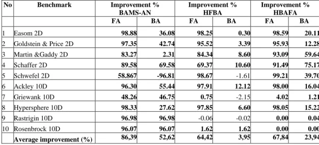
Table 5 presents the percentage of improvements in term of reducing NFE when comparing the enhanced variants of BA with the Standard BA.
searches with adaptive neighborhood search procedure in basic BA affects the results. The second best algorithm is HBAFA with the average percentage improvement of 67.84% and 23.94% compared to FA and BA, respectively. This variant of BA uses FA to improve the local search stage of Basic BA. On average, the capability to reduce the total NFE when applying Firefly Algorithm in initialization step of BA is 64.42% and
3.95% compared to FA and Standard BA respectively, which ranks HFBA in the third place.
Therefore, the enhanced variants of BA delivered a highly significant improvement in terms of overall performance. An interesting finding is that the introduced strategies and procedures helped BA to converge to good solutions quickly and robustly.
No Benchmark EA PSO FA BA2 BA1 BAMS-AN HFBA HBAFA
μE σE μE σE μE σE μE σE μE σE μE σE μE σE μE σE
1 Easom 2D 0.0000 0.0000 0.0000 0.0000 -0.7996 0.4039 0.0000 0.0000 0.0000 0.0000 0.0000 0.0002 0.0000 0.0000 0.0000 0.0000
2 Goldstein & Price 2D
0.0000 0.0000 0.0000 0.0000 0.0000 0.0000 0.0000 0.0000 0.0000 0.0000 0.0000 0.0001 0.0000 0.0000 0.0000 0.0000
3 Martin &Gaddy 2D
0.0000 0.0000 0.0000 0.0000 0.0000 0.0000 0.0000 0.0000 0.0000 0.0000 0.0000 0.0000 0.0000 0.0000 0.0000 0.0000
4 Schaffer 2D 0.0009 0.0025 0.0000 0.0000 0.0000 0.0000 0.0000 0.0000 0.0000 0.0000 0.0000 0.0000 0.0000 0.0000 0.0000 0.0000
5 Schwefel 2D 9.4751 32.4579 4.7376 23.4448 59.2194 64.4283 0.0000 0.0000 0.0000 0.0000 0.0003 0.0007 0.0000 0.0000 0.0000 0.0000
6 Ackley 10D 0.0000 0.0000 0.0000 0.0000 0.0010 0.0000 0.0000 0.0000 0.0000 0.0000 0.0000 0.0003 0.0000 0.0000 0.0000 0.0000
7 Griewank 10D 0.0210 0.0130 0.0199 0.0097 0.0178 0.0223 0.0089 0.0059 0.0120 0.0081 0.0000 0.0001 0.0120 0.0075 0.0127 0.0080
8 Hypersphere 10D 0.0000 0.0000 0.0000 0.0000 0.0000 0.0000 0.0000 0.0000 0.0000 0.0000 0.0000 0.0000 0.0000 0.0000 0.0000 0.0000
9 Rastrigin 10D 17.4913 7.3365 4.8162 1.4686 6.0692 2.7579 8.8201 2.2118 7.8601 2.1010 0.0002 0.0004 7.2632 2.1010 2.9848 0.8287
10 Rosenbrock 10D 61.5213 132.6307 1.7879 1.5473 10.1469 39.2052 0.0293 0.0068 0.1093 0.5627 0.0000 0.0003 0.1062 0.5637 0.0234 0.0022
Table 3: Accuracy of improved BA algorithms compared with FA and BA and other well-known optimization techniques.
No Benchmark EA PSO FA BA2 BA1 BAMS-AN HFBA HBAFA
Mean Std. Mean Std. Mean Std. Mean Std. Mean Std. Mean Std. Mean Std. Mean Std. 1 Easom 2D 36440 28121 97136 45642 189158.40 159102.21 3866 819 3326.9 415.2 2126 2260 3316.90 469.69 2658 858
2 Goldstein & Price 2D
5816 2259 4836 2361 57360 26870.34 2714 454 2658.4 383.4 1 522 660 2568.4 372.1 2332 479
3 Martin &Gaddy 2D
3248 1602 2512 781 12729.60 9644.23 2248 329 2180.3 363.7 2130 3034 1992.8 585.4 880 532
4 Schaffer 2D 219376 183373 35474 27151 121040.80 100516.67 27890 27335 41472.7 38237.9 12618 4330 37077.2 34805.7 10298 11777
5 Schwefel 2D
51468 133632 84572 90373 301726.40193824.47 5006 2110 3963.2 590.1 124108 0 4027.1 397.9 2390 1080
6 Ackley 10D 50344 3949 261608 9165 497459.20 4413.18 12186 3553 11836.2 3532.3 18398 7302 10402.2 516.4 9938 422
7 Griewank 10D
490792 65110 497714 16164 474366.40 43760.27 447064 126512 460894.8 102457.2 245 426,34 198326,6 470787.2 118.6821 455307 127061
8 Hypersphere 10D
36376 2736 223082 10872 356958.40 6627.86 8288 403 8212 425 5944 3926 7670.02 384.4 6962 332
9 Rastrigin 10D
500000 0 500000 0 500000 0.00 500000 0.00 500180 9.9 15 118 14186 500300 7.92 500000 0.00
10 Rosenbrock 10D
500000 0 500000 0 500000.00 0.00 500000 0 500000 0 19 642 6666 491924.1 57954.4 500000 0.00
5
Conclusion
In this paper, enhancements to the Bees Algorithm (BA) have been presented for solving continuous optimization problems. The basic BA was modified first to find the most promising patches, by using memory scheme in order to avoid revisiting previously visited sites, thus increasing the accuracy and the speed of the search, followed by adaptive neighborhood search procedure to escape from local optima during the local search process. This implementation is called BAMS-AN. The second improved version of BA, called HBAFA, uses Firefly Algorithm (FA) to update the positions of recruited bees in the local search part of BA, thus improving the convergence speed of the BA to good solutions. The third variant of BA, i.e. HFBA, developed a new strategy based on Firefly Algorithm (FA) to initialize the population of bees in the Basic BA, enhance the population diversity and start the search from more promising locations.
We evaluated the improved algorithms on several widely used benchmark functions and compared the results with those from the basic BA, FA and other state- of-the-art algorithms found in the literature. These benchmarks cover a range of characteristics including unimodal, multimodal, separable, and inseparable. The results have shown that BAMS-AN followed by HBAFA could track the optimal solution and give reasonable solutions most of the time. By including the improvements, both the search speed was improved and more accurate results were obtained. The comparisons among BA-based algorithms showed that BAMS-AN outperformed HBAFA, HFBA and the conventional BA. The experiments have also indicated that the improved variants of BA performed much better than the standard BA, PSO, FA and EA algorithms.
Testing the improved algorithms further on real world optimization problems and looking for algorithmic enhancements remains as future work.
6
References
[1] Mehmet Polat Saka, O. Hasançebi, and Zong Woo Geem. Metaheuristics in structural optimization and discussions on harmony search algorithm. Swarm and Evolutionary Computation, 28: 88-97, 2016. https://doi:10.1016/j.swevo.2016.01.005
[2] Lale Özbakir, and Pinar Tapkan. Bee Colony Intelligence in Zone Constrained Two-Sided Assembly Line Balancing Problem. Expert Systems with Applications, 38(9): 11947-11957, 2011. https://doi:10.1016/j.eswa.2011.03.089
[3] Marco Dorigo, and Gianni Di Caro. Ant Colony Optimization: A New Meta-heuristic. Proceedings of the 1999 Congress on Evolutionary Computation-CEC99 (Cat. No. 99TH8406), Wash-ington, DC, USA,
https://doi:10.1109/cec.1999.782657
[4] Dervis Karaboga, and Bahriye Akay. A Comparative Study of Artificial Bee Colony Algorithm. Applied Mathematics and Computation, 214(1): 108-132, 2009.
https://doi:10.1016/j.amc.2009.03.090
[5] Baris Yuce Michael S. Packianather, Ernesto Mastrocinque, Duc Truong Pham, and Alfredo Lambiase. Honey Bees In-spired Optimization Method: The Bees Algorithm. Insects, 4(4): 646-662, 2013.
https://doi:10.3390/insects4040646
[6] Duc Truong Pham, Afshin Ghanbarzadeh, Ebubekir Koç, Sameh Otri, Shafqat Rahim, and Muhamad Zaidi. The Bees Algorithm, A Novel Tool for Complex Optimization Problems. Proceedings of the Second International Virtual Conference on Intelligent production machines and systems (IPROMS 2006), Elsevier, Oxford. 454-459, 2006 https://doi.org/10.1016/j.engappai.2018.04.012 [7] Duc Truong Pham, and Marco Castellani. The Bees
Algorithm: Modeling Foraging Behavior to Solve Continuous Optimization Problems. Proceedings of
No Benchmark Improvement %
BAMS-AN
Improvement % HFBA
Improvement % HBAFA
FA BA FA BA FA BA
1 Easom 2D 98.88 36.08 98.25 0.30 98.59 20.11
2 Goldstein & Price 2D 97.35 42.74 95.52 3.39 95.93 12.28
3 Martin &Gaddy 2D 83.27 2.31 84.34 8.60 93.09 59.64
4 Schaffer 2D 89.58 69.58 69.37 10.60 91.49 75.17
5 Schwefel 2D 58.867 -96.81 98.67 -1.61 99.21 39.70
6 Ackley 10D 96.30 55.44 97.91 12.12 98.00 16.04
7 Griewank 10D 48.26 46.75 0.75 -2.15 4.02 1.21
8 Hypersphere 10D 98.33 27.62 97.85 6.60 98.05 15.22
9 Rastrigin 10D 96.98 96.98 -0.06 -0.02 0.00 0.04
10 Rosenbrock 10D 96.07 96.07 1.62 1.62 0.00 0.00
Average improvement (%) 86,39 52,62 64,42 3,95 67,84 23,94