Complexity Issues on Designing Tridiagonal Solvers on 2-Dimensional Mesh Interconnection Networks

Complexity Issues on Designing

Tridiagonal Solvers on 2-Dimensional

Mesh Interconnection Networks

Eunice E. Santos

Department of Electrical Engineering and Computer Science Lehigh University

We consider the problem of designing optimal and ef-ficient algorithms for solving tridiagonal linear systems with multiple right-hand side vectors on two-dimensional mesh interconnection networks. We derive asymptotic upper and lower bounds for these solvers using odd-even cyclic reduction. We present various important lower bounds on execution time for solving these systems including general lower bounds which are independent of initial data assignment, and lower bounds based on classifications of initial data assignments which classify assignments via the proportion of initial data assigned amongst processors. Finally, different algorithms are designed in order to achieve running times that are within a small constant factor of the lower bounds provided.

1. Introduction

In this paper, we consider the problem of de-signing algorithms for solving tridiagonal lin-ear systems. Such algorithms are referred to as tridiagonal solvers. A method for solving these systems, in which there is particular interest by designers, is the well-known odd-even cyclic re-duction method which is a direct method. Due to this interest, we chose to focus our atten-tion on odd-even cyclic reducatten-tion. Thus, our results will be applicable to tridiagonal solvers designed on a two-dimensional mesh utilizing cyclic reduction. Much research has been spent exploring this problem which deals with design-ing and analyzdesign-ing algorithms that solve these systems on specific types of interconnection networks 1, 5, 7, 8, 9, 10, 11] such as

hyper-cube or butterfly. However, very little has been

done on determining lower bounds for solving tridiagonal linear systems 4, 6, 10, 11]on any

type of interconnection network or on specific general parallel models 9]. Moreover, few of

these papers consider the case of multiple right-hand side(RHS)vectors and the authors know

of no papers which derive lower bounds on par-allel run-time for odd-even cyclic solvers with multiple RHS vectors.

The main objective of this paper is to present asymptotic upper and lower bounds on the run-ning time for solving tridiagonal systems with multiple right hand sides which utilize odd-even cyclic reduction on 2-dimensional meshes. Our decision to work with meshes is based on the simple fact that they are very common and fquently used interconnection networks. The re-sults obtained in this paper will provide not only a means for measuring efficiency of existing al-gorithms but also provide a means of pinpoint-ing algorithm design issues, data layouts and communication patterns in order to achieve op-timal or near-opop-timal running times.

While we have already derived results for tridi-agonal solvers with only a single vector on a 2-D mesh 10], the results were not easily adaptable

to multiple vectors. In fact, multiple vectors produced several layers of complexity towards analysis of this problem. Some of the interest-ing results we shall show include the followinterest-ing: The skewness in the proportion of data will sig-nificantly affect running time. Another inter-esting result is the proof on the threshold for

processor utilization. For some problem sizes, using common data layouts and straightforward communication patterns do not result in signif-icantly higher complexities than assuming that all processors have access to all data items re-gardless of communication pattern. In many cases, common data layouts can be used to ob-tain optimal running times. However, there is no one algorithm, data layout or communication pattern which will provide optimal run-times for all cases. In fact, we present more than 6 algorithms/subalgorithms which are needed in

order to show how to achieve optimal or near-optimal running times for all cases.

The paper is divided as follows. Section 2 con-tains a description of the 2-D mesh topology. In Section 3 we discuss the odd-even cyclic reduc-tion method for solving tridiagonal systems. In Section 4, we derive various important lower bounds on execution. First, we derive gen-eral lower bounds for solving tridiagonal sys-tems, i.e. the bounds hold regardless of data assignment. We follow this by deriving lower bounds which rely on categorizing data layouts via the proportion of data assigned amongst pro-cessors. Furthermore, we describe commonly-used data layouts designers utilize for this prob-lem. Lastly, we present a variety of algorithms and subalgorithms which will produce running times within a small constant factor of the lower bounds derived. Section 6 gives the conclusion and summary of results.

2. 2-Dimensional Mesh Interconnection Network

A mesh network is a parallel model on P pro-cessors in which propro-cessors are grouped as two types: border processors and interior proces-sors. Each interior processor is linked with exactly four neighbors. Each but for four bor-der processors have three neighbors. And the remaining four border processors have exactly two neighbors. More precisely:

Denote processors by somepi j where

1i j p

P

- For 1 < i j < p

P the four neighbors of pi jare pi+1j,pi;1j,pi j+1, andpi j;1

- Fori=1 and 1<j< p

Pthe three neigh-bors of pi j arepi+1j,pi j+1, and pi j;1

- For i = p

P and 1 < j < p

P the three neighbors ofpi jarepi;1j,pi j+1, andpi j;1

- Forj=1 and 1<i< p

Pthe three neigh-bors of pi j arepi+1j,pi;1j, andpi j+1

- For j = p

P and 1 < i < p

P the three neighbors ofpi jarepi+1j,pi;1j, andpi j;1

- Fori = 1 andj = 1 the two neighbors of

pi j arepi+1j, andpi j+1

- Fori = 1 and j = p

Pthe two neighbors ofpi jare pi+1j, and pi j;1

- Fori = p

Pandj = 1 the two neighbors

ofpi jare pi;1j, andpi j+1

- Fori= p

Pandj= p

Pthe two neighbors ofpi jare pi;1j, andpi j;1

Communication between neighbor processors require exactly 1 time step. By this, we mean that if a processor transmits a message to its neighbor processor at the beginning of time x, its neighbor processor will receive the mes-sage at the beginning of time x + 1.

More-over, we assume that processors can be receiv-ing transmittreceiv-ing]a message while performing a

local operation.

3. Odd-Even Cyclic Reduction Method

The Problem: Given M which is an NN

matrix, andRvectorsb1 b2bReach of size

N. For eachs( R), solvexswhereMxs =bs.

We assume that b1 b2bR can be stored in

one matrix B of size NR where the s th

col-umn of B represents vector bs. We make an

analogous assumption forx1 x2 xR.

More-over, we assume for the sake of simplicity that 1 < P = 2

2k

NR where k is an integer

and R = 2

r_{. An algorithm is simply a set of}

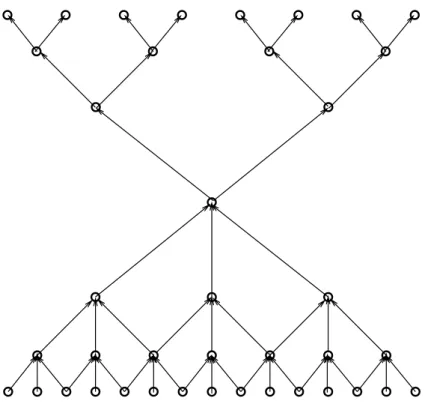
Fig. 1. Row dependency for odd-even cyclic reduction forN=15 andR=1.

components(algorithm, data layout,

communi-cation pattern)are needed in order to determine

running time.

Odd-even cyclic reduction 2, 3, 7]is a recursive

method for solving tridiagonal systems of size N = 2

n

;1. This method is divided into two

parts: reduction and back substitution.

The first step of reduction is to remove each odd-indexedxsi and create a tridiagonal system

of size 2n;1

;1. We then do the same to this

new system and continue in the same manner until we are left with a system of size 1. This requires n phases. We refer to the tridiagonal matrix of phase j as Mj and the vector as bjs.

The originalM andbs are denoted M0 andb0s.

The three non-zero items of each rowiinMjare denotedlji mji rij(left, middle, right). Below is

the list of operations needed to determine the items of rowiin matrixMj

(which we refer to

asMij.

ej_i=;

lj;1 i

mj;1 i;2

j;1

f_ij =;

rj;1 i

mj;1 i+2

j;1

lj_i=e j ilj

;1 i;2

j;1 r j i = f

j irj

;1 i+2

j;1

mj_i=m j;1 i +e

j irj

;1 i;2

j;1 +f

j ilj

;1 i+2

j;1

bj_{s i}=b j;1 s i +e

j ibj

;1 s i;2

j;1 + f

j ibj

;1 s i+2

j;1

The results in this paper assume that determin-ing values for each eji fij lji rji mji or bjs i are

atomic, i.e. if a processor is computing, for example, eji, then the processor must compute

all the operations to satisfy the equation foreji

given above.

Clearly, each system is dependent on the previ-ous systems. The lower half of Figure 1 shows the dependency between all theMj’s in the re-duction phase. The nodes in leveljof the figure represent the rows ofMj. A directed path from node a in level k to node b in level j implies that rowainMk_{is needed in order to determine}

the entries for row b in Mj. In fact, Figure 1 also pinpoints the dependencies between all the bjs i’s. Since there are no dependencies between

somebjs1i and someb y

s2z (wheres1 6= s2), the

only dependencies remaining are those between Mj_{’s andb}y

s’s. From the definition of the

prob-lem, we see that for eachs,bjs iis dependent on

In this paper, for simplicity, we assume that if an algorithm employs odd-even cyclic reduction, we assume that a processor computed items of whole rows of a matrix(i.e. the three non-zero

data items).

The back substitution phase is initiated after the system of one equation has been determined. We recursively determine the values of thexsi’s.

The first operation isxs_2n;1 =

bn;1

s2n;1 mn;1

2n;1

:For the

re-maining variablesxsi, letjdenote the last phase

in the reduction step beforexsiis removed, then

xsi =

bj;1 s i ;l

j;1 i xs_i

;2j ;1

;r j;1 i xs_i

+2j ;1

mj;1 i

:

Again, we are assuming the operations to com-pute thexsi’s are atomic forR = 1. However,

for the case ofR >1, we divide the operations

forxsi into the following atomic operations:

tempi=

lj;1 i xs_i

;2j ;1

+r j;1 i xs_i

+2j ;1

mj;1 i

and

xsi =

bj;1 s i

mj;1 i

;tempi:

Returning back to Figure 1, we see that the back substitution is represented by the top half of the graph. In essence, the entire tridiagonal sys-tem’s dependency graph isR+1 copies of the

graph in Figure 1 (one for the M matrix, and

the remaining for theRvectors)with some

ad-ditional edges. Clearly, for any two vectors of

b, their respective dependency graphs will not have any edges between them. In fact the only edges to be added are from the sub-dependency graph of M to every vector of b. In other words, for all vectors bs, each node in the M

sub-dependency graph will have an edge to the “mirror” node in the sub-dependency graph of

bs.

The serial complexity of this method is denoted byS(N R P)whereP =1. R =1 is a special

case, i.e.

S(N 1 1)=19N;14 log(N+1);4:

ForR>1,

S(N R 1)=15N;10n;5+M(6N;4n;1):

In Section 4, we derive several important lower bounds on running time for odd-even cyclic reduction algorithms on 2-D mesh networks. Specifically, we derive general lower bounds in-dependent of data layout, lower bounds which are based on categorization of data layouts, and lower bounds on running time for common data layouts for this problem. In Section 5.6 we present optimal algorithm running times on 2-d mesh topologies.

4. Lower bounds for Odd-Even Cyclic Reduction

Definition 4.1. The class of all communica-tion patterns is denoted byC. The class of all

data layouts is denoted byD. A data layout D

is said to be a single-item layout if each non-zero matrix-item is initially assigned to a unique processor.

In the following sections we shall provide lower bounds based on certain types of data layouts as well as general lower bounds. The lower bounds hold regardless of the choice of communication pattern.

4.1. A General Lower Bound for Odd-Even Cyclic Reduction

In this subsection we assume the data layout is the one in which each processor has a copy of every non-zero entry ofM0andb0_s. We denote this layout by ¯D. Since ¯Dis the best data lay-out possible, a lower bound based on this data layout will provide a general lower bound.

Remark 4.1. We will denote the (parallel) com-putation lower bound for odd-even cyclic reduc-tion of size N and R and utilizing P processors by S(N R P).

Remark 4.2. Let A be an odd-even cyclic re-duction algorithm. A computation lower bound for A, given P processors and assuming none of the P processors are totally idle is S(N R P)=

Ω( NR

Theorem 4.1. Let A be an odd-even cyclic re-duction algorithm. The following is a lower bound for A regardless of data layout and com-munication pattern:

8 > > <

> > :

max(S(N R P) p

(P=R))=Ω( NR

P +logN +

p

(P=R)) if PRN 2 3

max(S(N R RN 2

3))=Ω(N 1

3) otherwise

Proof. We will begin by assuming that all P processors will be used in computation and/or

communication. Clearly, S(N R P) is a lower

bound for the problem. Furthermore, we see that there are groups of processors which work together in order to solve the items in the de-pendency graph of M or in any of the bs’s

graphs. Denote these(not necessarily disjoint)

groups of processors byM1,M2 Mz. Let

P0

= maxi z

jMij(min(N P)). Since these

processors must ultimately produce only one row of M in the back substitution phase, it is clear there is some type of “all-to-one broad-cast” of P0 processors in order to complete the

back-substitution phase ofM and/orbs. Thus,

on a two-dimensional mesh, this will require communication of at leastp

P0. Moreover, this

will also require computation of at least _PN0.

Therefore, a lower bound, assuming allP pro-cessors are used, is max(S(N R P)

N P0

p

P0 ).

This leads to the fact thatP0

=max(1 P

R)in

or-der to minimize the lower bound. Furthermore, we see that using more than Ω(RN

2

3)

proces-sors, will reduce efficiency; i.e. the threshold for procesor utilization isΩ(RN

2 3).

In Section 5.6 we will provide optimal algo-rithms, i.e. the running times are within a small constant factor of the lower bounds. There-fore, we note that our results show that when P is sufficiently large, i.e. P = Ω(RN

2 3)

us-ing more thanRN23 processors will not lead to

any substantial improvements in running time if utilizing data layout ¯D.

4.2. Lower Bounds forOon c

P-data layouts

Many algorithms designed for solving tridiago-nal linear systems assume that the data layout is

single-item and that each processor is assigned roughly _P1thof the rows ofM0 _{and the items of}

b where P is the number of processors avail-able. However, in order to determine whether skewness of proportion of data has an effect on running time and if so, exactly how much, we classify data layouts by initial assignment pro-portions to each processor. In other words, in this section, we consider single-item data lay-outs in which each processor is assigned at most a fraction _Pc of the rows of M and items of b where 1cP(

NR+N;P+1 NR+N

).

Definition 4.2. Consider c where 1 c <

P(

NR+N;P+1

NR+N

). A data layout D on P

processors is said to be a _Pc-data layout if (a) D is single-item,

(b) no processor is assigned more than a frac-tion _Pc of the rows of M0or items of b,

(c) at least one processor is assigned exactly a fraction_Pc of the rows of M0_{or items of b, and}

(d) each processor is assigned at least one row of M0or items of b.

Denote the class of _Pc data layouts byD( c P).

Theorem 4.2. If D 2D( c

P), then for any A 2 Ofor R vectors, a lower bound is

max(S(N R P) p

P 8

NRc 6P ) =Ω(

NR

P +logN + p

P+

NRc P )

Proof. The computational lower bound must also be a lower bound for the problem regardless of communication. Thus S(N R P)is a lower

bound. Moreover, since at least one processor is assignedNRc_P pieces of data, this processor(

de-noted as p0) can either choose to use that data

item in a binary arithmetic operation or send out the item to another processor. Therefore, it is clear that NRc_6P must also be a lower bound. We will now describe the argument for why

p P 8

must also be a lower bound. We will use a contradiction argument.

Consider any two data items fromMand/orB.

are both required by some computation in order to provide final solutions. Clearly, any initial data item ofM, i.e. M0 _{will be related to any}

other initial item ofM. Suppose the

p P

8 is not a

lower bound, this implies that any two proces-sors which are both assigned initial items ofM cannot be more than or equal to a distance of

p P

4 from each other on the 2-D mesh.

Further-more, consider a processor pwhich computes Mn;1. Processorpwill require data from all of

the items ofM0. Clearly, only processors which are within at most a distance of

p P

8 ;1 can be

as-signed items fromM0_{. Furthermore, expanding}

the distance from

p P 8 ;1 to

p P

4 ;2 frompwill

now contain all the processors which will uti-lize any item fromM0_{for computation. Finally}

expanding the distance from pto 3

p P

8 ;3 will

represent all the processors that are assigned data items from not only M0 _{but also items of}

B0 _{which are related to any item inM}0_{. Every}

processor is assigned at least one initial piece of data and the layout is single-item. Moreover, every item inB0is related to at least one item of M0. Thus, every processor assigned an item of B0orM0must be inside this region. However, the region does not include all the processors in the mesh. Therefore, this is a contradiction.

Analyzing the result given in the above theorem, we see that_P1-data layouts will result in the best lower bounds for this class of data layouts, i.e. :

Corollary 4.1. If D 2 D( 1

P), then for any

A2Ofor R vectors, a lower bound is

max(S(N R P) p

P)=Ω(

NR

P +logN+ p

P)

Comparing results against the general lower bound, we see that for sufficiently largeN (i.e.

N >> P, or more precisely P R(N) 2 3),

the lower bound for _P1-data layouts is precisely equal to the general lower bound. The com-plexity of any algorithmA2 O using a

1 P-data

layout isΩ(logN+ NR

P + p

P). In Section 5.6,

we present algorithms that are within a small constant factor of the bounds presented in this and previous subsections.

5. Optimal Algorithms, Data Layouts, and Communication Schedules

In this section, we design the algorithms which will produce running times which are within a small constant factor of the lower bounds de-rived in the last section. We begin by dis-cussing the data layouts we plan to use. We follow this with a discussion of some of the communication schedules(mostly dealing with

distribution/broadcast of the data to processors

that require this information for computation).

Lastly, we present the optimal algorithms along with their running times. We will discuss under which circumstances one algorithm should be used over another in order to achieve optimal or near-optimal running times.

5.1. Definitions of Data Layouts

In the previous sections, we have derived var-ious lower bounds on running time for tridi-agonal solvers which utilize odd-even cyclic reduction on a 2-dimensional mesh intercon-nection topology. In order to design algorithms which are within a constant factor of these lower bounds, we must determine which types of data layouts we will use. In this section, we present definitions on data layouts in order to use these layouts in the next subsections in our algorithm designs.

We would like to point out that while we can easily use the best data layout ¯D to obtain the general lower bounds, in this section we will present data layouts which are not so powerful but which still achieve the lower bounds stated. In fact, in the cases whereN >>P, no

proces-sor is assigned more thanO( NR

P )data items.

We begin by presenting partial layouts and in each subsection, we discuss a data layout we will utilize in our optimal algorithms.

Definition 5.1. Let P be an integer where1

PN and2 i

;1P<2 i+1

;1. A data layout

on P processors, p1 pP, is an

M-replicative-blocked data layout if for all j<2 i;1, p

jis

as-signed the nonzero items in rows(j;1)2 n;i

+1

to(j+1)2 n;i

;1of M

0_{. We denote this layout}

Definition 5.2. Let P be an integer where1

PN and2 i

;1P<2 i+1

;1. A data layout

on P processors, p1 pP, is anbs

-replicative-blocked data layout if for all j < 2 i;1, p

j is

assigned bs l where (j ; 1)2 n;i

+ 1 l

(j+1)2 n;i

;1. We denote this layout by Db

sP.

Definition 5.3. Let P be an integer where1

P N and P = 2

i_{. A data layout on P}

pro-cessors, p1 pP, is an M-single-item-blocked

data layout if (a) for all j<P;1, pjis assigned

the nonzero items in rows(j;1) N P;1

+1to j N P;1

of M0_{, (b) p}

P;1is assigned the nonzero items in

rows(P;2) N P;1

+1to(P;1) N P;1

;1of M 0_,

and (c) pP is assigned the nonzero items in row

N of M0_{. We denote this layout by D}0 M P.

Definition 5.4. Let P be an integer where1

PN and2 i

;1P<2 i+1

;1. A data layout

on P processors, p1 pP, is anbs

-single-item-blocked data layout (a) for all j < P;1, pj is

assigned the vector items(j;1) N P;1

+1to j N P;1

ofbs, (b) pP;1is assigned the nonzero items in

vector items(P;2) N P;1

+1to(P;1) N P;1

;1

ofbs, and (c) pP is assigned the vector item N

ofbsp. We denote this layout by D0

bsP.

5.1.1. Data Layout 1

IfPRN 2

3 then we will only useR22b

n;1 3 c

pro-cessors, and, in this case, we will simply assume P=R2

2b

n;1 3 c.

This data layout will be utilized in order to achieve the general lower bounds whenRP.

We begin by partitioning the processors intoR groups of P_R = 2

2k;r processors. For the sake

of simplicity, we will assume that r is even. TheseRgroups will be referred to asPi jwhere

1i j p

R.

The processors assigned to group Ps t are pi j

where (s ; 1)2 k;

r

2 + 1 i s2

k;

r

2 and

(t;1)2 k;

r

2 +1jt2

k;

r 2.

We will create a new notation for the mesh pro-cessors in order to utilize the partial data layouts defined in this section. Consider the processors in groupPs t, these processors will be denoted

byps t₁ ps t₂ p s t

P

R wherep

(s;1)2

k;

r

2+i(t;1)2

k;

r 2+j

is denoted by

- ps t

(i;1) p

P=R+j

ifiis odd

- ps t

(i;1) p

P=R+ p

P=R;j+1

ifiis even

For each groupPs t, we will allocate the items of

Musing data layoutD_MP

R. Moreover, this group

of processors will be allocated vectorb

(s;1)

P R+t

using data layoutD_b

(s;1)

P r

P R.

5.1.2. Data Layout 2

This data layout will be utilized in order to achieve the general lower bounds whenR>P.

We begin by partitioning the assignment of the

bs vectors to theP processors. Each processor

will be assigned R_P whole vectors. In particular pi jwill be assigned the items in vectorsblwhere

(i;1) R p

P+(j;1) R

P+1l(i;1) R p

P+(j) R P:

Moreover, every processor will be assigned the items in matrixM.

5.1.3. Data Layout 3

This is a single-item data layout and will be utilized in order to achieve the single-item data layout lower bounds whenP <N.

We will create a new notation for the mesh pro-cessors in order to utilize the partial data layouts defined in this section. The processors will be denoted by p1 p2 pP where p

i j _{is denoted}

by - p

(i;1) p

P+j

ifiis odd - p

(i;1) p

P+ p

P;j+1

ifiis even

We will allocate the items ofM using data lay-outD0

M P. Moreover, the processors will be

al-located each vectorbs using data layoutD0

5.1.4. Data Layout 4

This is a single-item data layout and will be utilized in order to achieve the single-item data layout lower bounds whenP>N andRP.

We begin by partitioning the processors into R groups of P_R = 2

2k;r processors. These R

groups will be referred to asPiwhere 1 i

R. IfR

p

Pthen the processors assigned to group

Pl are pi j where (l;1)2 k;r

+1 i l2

k;r

and 1j p

P.

We will create a new notation for the mesh pro-cessors in order to utilize the partial data layouts defined in this section. Consider the processors in group Pl, these processors will be denoted

by pl

1 pl2 p l

P

R where p(l;1)2

k;r +i j

is denoted by

- pl (i;1)

p P+j

ifiis odd - pl

(i;1) p

P+ p

P;j+1

ifiis even

However, if R > p

P then the processors as-signed to groupPl where l = x

R p

P +y are pi j

wherei =x+1 and(y;1) P

R +1jy P R.

We will create a new notation for the mesh pro-cessors in order to utilize the partial data layouts defined in this section. Consider the processors in group Pl, these processors will be denoted

by pl

1 pl2 p l

P

R where p

(l;1)2

k;r

+i j is denoted

bypl

(i;1) p

P+j

.

Regardless of the size of R, for groupP1, we

will allocate the items of M using data layout D0

M P_R. Moreover, each group Pl will be

allo-cated vectorblusing data layoutD0

b_l P_R. Clearly,

this is a c

P-data layout wherecis constant.

5.1.5. Data Layout 5

This is a single-item data layout and will be utilized in order to achieve the single-item data layout lower bounds whenR>P>N.

We begin by partitioning the assignment of the

bs vectors to thePprocessors. Each processor

will be assignedR_P full vectors. In particularpi j

will be assigned the items in vectors bl where

(i;1) R p

P+(j;1) R

P+1l(i;1) R p

P+(j) R P:

Moreover, processor p1 1 will be assigned the

items in matrix M. Clearly, this is a _Pc-data layout wherecis constant.

The data layouts presented in this subsection will be used to design optimal or near-optimal algorithms for solving tridiagonal systems on a 2-dimensional mesh. We again note that while we could have simply assumed the best data lay-out for designing our algorithms to achieve the general lower bounds, we instead have listed data layouts in which no processor has been assigned more than O(

NR

P ) initial data items.

Furthermore, we have presented several single item data layouts which we will be using in our optimal algorithm designs in later subsections. In the following subsection, we present some communication schedules which we will use in our algorithms designs. These schedules are used to address data redistribution.

5.2. Communication Schedules

For some of the algorithms we will design in the next subsection, it is important that we are able to redistribute the data from one layout to another. In this section, we present communi-cation schedules which do the needed redistri-butions.

5.3. Schedule 1

In this communication schedule, we are redis-tributing data layout 3 into the layout in which the matrixMis distributed usingDM Pand each

bs is distributed using DbsP. Clearly, only neighbor processors(as ordered in the data

lay-out discussion for 3)need to communicate.

This would be accomplished by running the fol-lowing:

For alljP;2, processorspjdo in parallel

send all initially assigned data items to processorpj+1

send all initially assigned data items to processor pj;1

Running Time: O( RN

P ).

5.4. Schedule 2

In this communication schedule, we are redis-tributing data layout 4 into the layout in which the matrix M is distributed to each group us-ing layout D_MP

R. Moreover, we also wish to

redistribute the b vectors such that instead of D0

bP_R, we wish the distribution to beDb P_R. Two

slightly different schedules for this redistribu-tion are needed: one for R

p

P and one for R>

p

P.

We will discuss the schedule forR p

P. The redistribution schedule for the other case is very similar and, for brevity, we will omit its discus-sion.

ConsiderR p

P. We begin by redistributing so that each group is assigned the matrixM us-ing D0

M P_R. Clearly, only processors above and

below(on the mesh)a processor need the same

data to communicate. Collecting the data items ofMin each column to the first processor in the column and then sending out the information to every other processor in the column would effectively accomplish the first step of the re-distribution. The remaining redistributions can be easily taken care of using Schedule 1 above. This would be accomplished by running the fol-lowing:

For allj p

Pdo in parallel For all 2<i

p P

R every processor pi jdo

in parallel

send all initial data items ofM top1j (pipelined broadcast)

p1jdo a one to all(pipelined)broadcast of

the items ofM to processorsp2j p p

P j.

For each groupPldo in parallel

Run schedule 1 for the assigned vector Run schedule 1 forM

Running Time: O( RN

P + p

P).

5.5. Schedule 3

In this communication schedule, we are redis-tributing data layout 5 into the layout in which the matrix M is distributed to every proces-sor. This is simply a “one-to-all broadcast” of 3(N ;1) items. Clearly, this can be

accom-plished in O(N ;1+ p

P) steps. Due to the

assumptions made in layout 5, the running tims isO(

NR P +

p

P+logN).

5.6. The Optimal Algorithms

In the previous subsections, we have discussed the data layouts and some communication re-distribution schedules we plan to use in our al-gorithms. In this section, we present the algo-rithms which will produce running times within at most a small constant factor of the lower bounds presented in the previous section.

5.6.1. SubAlgorithm 1 for Best Data Layout

This algorithm solves a tridiagonal system by sequentially solving values based on values it has already computed and not sent from another processor. This Subalgorithm will be a building block for the full algorithms.

Assume y of the vectors of b are assigned to this group of P0

= 2

q _{processors. Moreover,}

assume the processors are ordered using the or-dering given in data layout 3. The items of row iof leveljare considered to belji rij mjiandbjs i (of ally vectors). Lastly, we will utilize only

P0

;1 processors.

SubAlgorithm1 forData LayoutD¯ Every processorpi(1i<2

q

)do in parallel :

fors=1 ton;qdo

forz=2 n;q;s

(i;1)+1to

2n;q;s

(i+1);1do

compute(serially)the items of rowzof

levels

send items of rowiof leveln;qtopi +1and

/* ifi=P 0

;1 do not send, and ifi=1

do not receive */

send items of rowiof leveln;qtopi ;1and

receive frompi+1 /* ifi=2

q

;1 do not receive, and ifi=1

do not send */

fors=1 toq;1do

if ₂is is an integerthen

compute the items of row 2;s

iof level n;q+s

ifs 1

2logP then

send items of rowi2;sof leveln

;q+s

topi+2

s routed through the path

(pi

+1 pi+2 pi

+k pi+k+1 pi

+2

s

;1 )

and received from pi;2

s

/* ifi+2s>2 q

;1 do not send, and

ifi;2 s

<1 do not receive */

send items of rowi2;sof leveln

;q+s

topi;2

s routed through the path

(pi

;1 pi;2 pi

;k pi;k;1 pi

;2

s

;1 )

and received from pi+2

s

/* ifi+2s>2 q

;1 do not receive,

and ifi;2 s

<1 do not send */

elses= 1

2logP+k

send items of rowi2;sof leveln

;q+s

topi+2

s routed through the path

(p i+

p P pi+2

p P p

i+j p

P pi+(j+1) p

P

p i+(2

k

;1) p

P)and received frompi ;2

s

/* ifi+2s>2 q

;1 do not send,

and ifi;2 s

<1 do not receive */

send items of rowi2;sof leveln

;q+s

topi;2

s routed through the path

(p i;

p P pi;2

p P p

i;j p

P pi;(j;1) p

P

p i;(2

k

;1) p

P)and received frompi +2

s

/* ifi+2s>2 q

;1 do not receive,

and ifi;2 s

<1 do not send */

For back substitution, if piwas the last

processor to handle items of rowj then picomputes allxsi wherebsis

assigned to pi(and if necessary,

send and receive appropriate values of allxsm)

Running Time: O( Ny P0

+ylogP 0

+ p

P0 )

5.7. Algorithm 1 for Data Layout 1

This data layout is used whenRP. This

algo-rithm is simply solving the tridiagonal system with one vector. We have partitioned the pro-cessors intoRgroups. Since the best data layout actually is not needed for subalgorithm 1 and in fact our data layout is sufficient, we simply call SubAlgorithm 1 for each group in parallel with P0

= P

R,y =1. Therefore the total running time

isO( NR

P +log P R+

q P

R)=O( NR

P +logN+ q

P R):

As we stated in the subsection defining Data Layout 1, if P RN

2

3, we simply assume

P=RN 2

3. Therefore the running time is clearly

O(N 1 3).

5.8. Algorithm 2 for Data Layout 2

This data layout is used whenR > P. This

al-gorithm is simply sequentially solving the tridi-agonal system with R_P right-hand side vectors. We have partitioned the vectors intoP groups. Each processor in parallel, serially solves their assigned system. Therefore the total running time isO(

NR

P +logN)=O( NR

P +logN+ q

P R):

5.9. Algorithm 3 for Data Layout 3

This algorithm first calls schedule 1, then it sim-ply solves the tridiagonal system withRvectors. We consider the caseP<

N

logN. Since the best

data layout is actually not needed for subalgo-rithm 1 and in fact our data layout is sufficient

(after schedule 1), we simply call SubAlgorithm

1 withP0

= P,y = R. Therefore the total

run-ning time is the time for Schedule 1 plus the time for Subalgorithm 1: O(

NR

P +RlogN+ p

P):

Since P < N

logN then the run-time is clearly

O( NR

P + p

P+logN).

For the case where _logN_N P N,

in the last phases of reduction and the first phases of back substitution are replicated so that at least half the processors are always work-ing. This will produce a running time of: O(

NR

P +logN+ p

P):

5.10. Algorithm 4 for Data Layout 4

This algorithm first calls schedule 2 then it is simply solving the tridiagonal system with one vector. We have partitioned the processors into Rgroups. Since the best data layout is actually not needed for subalgorithm 1 and in fact our data layout is sufficient (after schedule 2), we

simply call SubAlgorithm 1 for each group in parallel withP0

= P

R,y=1. Therefore the total

running time isO( NR

P +logN + p

P):

5.11. Algorithm 5 for Data Layout 5

This algorithm first calls schedule 3, then it is simply sequentially solving the tridiagonal sys-tem with R_P right-hand side vectors. We have partitioned the vectors into P groups. Each processor in parallel, serially solves their as-signed system. Therefore the total running time isO(

NR

P +logN+ p

P):

In this section, we designed algorithms for each of the data layouts which cover all problem sizes. Analyzing the running times of our al-gorithms, we see that they are all within a small constant factor of the lower bounds provided. In particular, the algorithms for Data Layouts 1 and 2 satisfy the general lower bounds. The algorithms for the remaining Data Layouts all satisfy the single-item bounds. Moreover, an-alyzing the design of the algorithms, we see that to achieve the single-item bounds simply requires redistribution of a single-item layout to the layouts used to achieve the general lower bounds. Furthermore, no layout assigned any processor more thanO(

NR

P )initial data items.

6. Conclusion

In this paper we examined the problem of designing optimal tridiagonal solvers on 2-dimensional mesh interconnection networks

with multiple right hand sides using odd-even cyclic reduction. This is the first paper to have tackled and solved this problem asymptotically. We were able to derive asymptotic lower bounds on the execution time. Moreover, we were able to provide algorithms whose running times dif-fer by only a small constant factor of these lower bounds.

Specifically, we proved that the complexity for solving tridiagonal linear systems regardless of data layout(i.e. a general parallel lower bound

on a 2-dimensional mesh)isΩ(N 1

3)whenP =

Ω(RN 2

3)else the bound isΩ( NR

P +logN+ q

P R).

This shows that utilizing more than Ω(RN 2 3)

processors will not result in any substantial run-time improvements. In fact, utilizing more pro-cessors may result in much slower run-times. When we added the realistic assumption that the data layouts are single-item and the num-ber of data items assigned to a processor is bounded, we derived lower bounds for classes of data layouts. The asymptotic lower bound is

Ω( NR

P +logN+ p

P). We provided three types

of data layouts which provided optimal running times. In other words, we showed that the best types of layouts in general are those in which either (a) each processor is assigned an equal

number of rows ofM0andb,(b)the processors

are grouped intoRgroups in which every group is assignedP_R of the vectors, or(c)each

proces-sor is assignedR_Pwhole vectors ofb. Therefore, we see that the skewness of proportion of data will significantly affect performance. Compar-ing the lower bounds for the c

P-layouts with the

general lower bounds, we see that restricting the proportion of data items assigned to a processor to NR_P does not result in a significantly higher complexity than assuming all processors have all the data items for sufficiently large N (i.e.

PRN 2 3).

Lastly, we show that there are algorithms, data layouts, and communication patterns whose run-ning times are within a constant factor of the lower bounds provided. This provides us with theΘ-bounds stated above.

data layout, i.e. the data layout in which every processor is assigned all the data items, we did not. We presented two data layouts in which no processor was assigned more thanO(

NR P )data

items. Two types of algorithms produce optimal running times: (a)algorithms in which

proces-sors are partitioned into R sets such that each set is in essence an independent tridiagonal sys-tem, or(b)algorithms in which each processor

sequentially solves R_P of the vectors.

As stated previously, three different data lay-outs were provided in order to design optimal algorithms for single-item layouts. The three types of algorithms are: (a) algorithms which

in essence utilize block layouts and solve the tridiagonal system R times. (b) algorithms in

which processors are partitioned intoRsets such that each set is in essence an independent tridi-agonal system, or(c)algorithms in which each

processor sequentially solves R_P of the vectors. For (b)-(c), the algorithms provided are very

similar to those to achieve the optimal running times (regardless of data layout). In fact, the

difference in run-time is primarily the need to do redistributions of data in order to run the optimal algorithms.

Finally, it is worthwhile to observe that for suf-ficiently largeN, the single-item lower bounds are asymptotic to the general lower bound.

References

1] C. AMODIO AND N. MASTRONARDI, A parallel version of the cyclic reduction algorithm on a hypercube,Parallel Computing, 19, 1993.

2] D. HELLER, A survey of parallel algorithms in numerical linear algebra, SIAM J. Numer. Anal., 29(4), 1987.

3] A. W. HOCKNEY AND C. R. JESSHOPE, Parallel Computers, Adam-Hilger, 1981.

4] S. L. JOHNSSON, Solving tridiagonal systems on ensemble architectures,SIAM J. Sci. Stat. Comput., 8, 1987.

5] S. P. KUMAR, Solving tridiagonal systems on the butterfly parallel computer, International J. Super-computer Applications, 3, 1989.

6] S. LAKSHMIVARAHAN ANDS. D. DHALL, A Lower Bound on the Communication Complexity for Solv-ing Linear Tridiagonal Systems on Cube Architec-tures, InHypercubes 1987, 1987.

7] S. LAKSHMIVARAHAN ANDS. D. DHALL, Analysis and Design of Parallel Algorithms : Arithmetic and Matrix Problems, McGraw-Hill, 1990.

8] F. T. LEIGHTON,Introduction to Parallel Algorithms and Architectures: Arrays-Trees-Hypercubes, Mor-gan Kaufmann, 1992.

9] E. E. SANTOS, Optimal Parallel Algorithms for Solving Tridiagonal Linear Systems, In Springer-Verlag Lecture Notes in Computer Science #1300 (Proceedings of Euro-Par), 1997.

10] E. E. SANTOS, Optimal Tridiagonal Solvers on Mesh Interconnection Networks InSpringer-Verlag Lecture Notes in Computer Science #1557 (Pro-ceedings of ACPC), 1999.

11] E. E. SANTOS, Solving Tridiagonal Linear Systems on a Torus Proceedings of the International Con-ference on Parallel and Distributed Processing and Techniques, 1998.

Received: May 15, 1999 Accepted in revised form:January 21, 2000

Contact address: Eunice E. Santos Department of Electrical Engineering and Computer Science

19 Memorial Drive West Lehigh University Bethlehem, PA 18015 phone:+1(610)758-4517

Fax:+1(610)758-6279

[email protected]. edu