Vol. 1, No. 1, 2008, (4-37)
ISSN 1307-5543 – www.ejpam.com
Honorary Invited Paper
Multivariate Regression Models with Power Exponential Random
Errors and Subset Selection Using Genetic Algorithms With
Information Complexity
Minhui Liu1, Hamparsum Bozdogan2,∗
1Department of Statistics, Operations and Management Science, University of Tennessee, 2Stokley Management Center, Knoxville Tennessee, 37996-0562 U.S.A.
Abstract. In this paper we introduce and develop two different novel multivariate regression models with Power Exponential (PE) random errors for the first time. Our first model assumes that the observations are independent and the second model assumes that the observations are dependent. These two models coincide only when the shape parameter of the multivariate Power Exponential (MPE) distribution is equal to one which corresponds to the multivariate normal distribution. We develop method of moments (MOM) and the maximum likelihood (ML) methods to estimate the model parameters. The model selection criteria such as AIC and ICOMP(IFIM) for both models are derived. Two simulation examples and a real example on a benchmark data set are given to show the applications of these two models in subset selection of the best predictors. A genetic algorithm (GA) approach is used to obtain the estimates of the model parameters and to carry out the subset selection of the best predictors under these two different model types.
Key words: Multivariate Power Exponential Distribution, Multivariate Regression, AIC, ICOMP, Model Selection, Genetic Algorithm.
1. Introduction and Objectives
During the past fifty years, multivariate normal distribution has enjoyed a significant role in the development of many important multivariate modeling techniques including the multivariate regression models. In many practical applications such as in behavioral and social sciences, bio-metrics, chemobio-metrics, econobio-metrics, environmental sciences, and financial modeling to name a few, we cannot any longer assume the multinormality on the set of dependent variables or the random error term of the model. Real data often show significant departures from normality and normality may not be tenable, especially when the tails are thicker or thinner than those of nor-mal distributions. For this reason, to achieve more flexibility in statistical modeling and model selection, and to robustify many multivariate statistical procedures, the purpose of this paper is to develop novel techniques in multivariate regression models for nonnormal data under the general class of: Multivariate Power Exponential (PE) distributions by broadening the usual multivariate normal assumption on the random errors under various assumptions. In regression models, the
∗Corresponding author.Email address: [email protected](H. Bozdogan)
random error terms are generally assumed to be normally distributed. However, since data of-ten are non-normal, the normality assumption is not always of-tenable especially when the tails are thicker or thinner than those of normal distributions. The Power Exponential (PE) distribution family which is introduced by Subbotin ( [32]) and popularized by Box and Tiao ( [6]), has been used in modeling economic and financial data as a generalization of normal distribution in recent years (e.g. [28, 33, 34]). G´omez-Villegas and S´a nchez-Manzano et al. ( [20, 31]) proposed multi-variate and matrix generalizations of the PE family of distributions and studied their properties in relation to multivariateElliptically Contoured(EC) distributions.
Zeckhauser and Thompson ( [36]) were probably the first who attempted to study the simple multiple linear regression model with PE error terms in a short but an incomplete paper. Liu and Bozdogan ( [23]) developed a GA on GA (or GA engineering) approach for PE multiple regression and subset selection of variables with information-theoretic complexity (ICOMP) criterion. The closed form expressions of the inverse Fisher Information Matrix (IFIM) and ICOMP(IFIM) for PE multiple linear regression models were also given. Finding proper criterion or measure for the comparison of competing models is important to select correct regression models. AIC-type criteria ( [2–5]) are the most widely used information-based criteria for model selection in recent years. However, the penalty term used in AIC-type criteria is insufficient to measure the model complexity which has been cited by many authors (see, e.g. [29]). Bozdogan’s ICOMP criteria ( [7,9,10,12–14]) improve AIC-type criteria by using an information-theoretic measure of“overall”
model complexity based on the generalized covariance complexity index of van Emden ( [16]). ICOMP(IFIM) is the most general form of ICOMP.
In this paper, we extend the work of Liu and Bozdogan ( [23]) and study the multivariate regression models with PE random errors under various assumptions. As a short hand notation, we abbreviate these models as MVPER models. We develop and use the genetic algorithms (GAs) for both the parameter estimation of the models and for subset selection of best predictors with information criteria as our fitness function. We note that, in the literature, this work seems to be the first to attempt to study MVPER models utilizing modern optimization techniques such the GAs and information criteria as our fitness function. More specifically, we consider the multivariate regression model:
Yn×p =Xn×qBq×p+En×p, p+q ≤n, rank(X) =q (1.1)
where Y = [y1,y2,· · · ,yp] = [y(1),y(2),· · ·,y(n)]0 is the matrix of nobservations on p re-sponse variables.X = [x1,x2,· · · ,xq] = [x(1),x(2),· · · ,x(n)]0is the matrix of(n×q)constant terms on non-stochastic predictor variables,B = [b1,b2,· · · ,bp] = [b(1),b(2),· · ·,b(q)]0 is the coefficient matrix andE = [ε1, ε2,· · ·, εp] = [ε(1), ε(2),· · ·, ε(n)]0 is the unobservable random error term matrix. The error terms are assumed to be multivariate PE rather than normal. Ap-plying thevector operatorV ec(·)( [30, p.21]) to (1.1), the multivariate regression model can be transformed to a univariate regression problem given by
V ec(Y0) =V ec(B0X0) +V ec(E0) = (X⊗Ip)V ec(B0) +V ec(E0) (1.2)
or
whereynp×1 = [y0
(1),y0(2),· · ·,y0(n)]0,bpq×1 = [b0(1),b0(2),· · ·,b0(q)]0andεnp×1 = [ε0(1), ε0(2),· · · , ε0(n)]0.
Ip is the(p×p) dimensional identity matrix. ⊗isKronecker productoperator ( [30, p.12]). In this paper, we letV ec0(·)denote(V ec(·))0.
The rest of the paper is organized as follows. In Section 2, we introduce the multivariate PE distribution. In Section 3, we study Type I MVPER model and in Section 4 we study Type II MVPER model which takes the dependency structure of the data into account. Section 5 gives the derivation of AIC and ICOMP(IFIM) for these two types of MVPER models. Section 6 outlines and presents the general background of the Genetic Algorithms (GAs). In Section 7, we give two simulation examples and a real model selection example on a benchmark macro-economic data in subset selection of best predictors under both the Type I and Type II MVPER models to illustrate the versatility of our new approach. Section 8 concludes the paper.
2. Multivariate PE Distributions
A random variablezis PE distributed if the density function ofzis
f(z;µ, σ, β) = 1
σΓ
³
1 + 1
2β ´
21+21β
exp
Ã
−1
2
¯ ¯ ¯ ¯z−σµ
¯ ¯ ¯ ¯
2β!
, (2.1)
where the parameters−∞< µ < ∞andσ >0are location and scale parameters, respectively, andβ >0is the shape parameter, which is related to thekurtosis parameter. A family of unimodel symmetric curves with different shapes for different values ofβcan be represented by the above density. When β = 0.5, the Laplace distribution, and when β → ∞ the Uniform distribution arises. Particularly whenβ = 1, the density becomes normal distribution. So PE distribution can be seen as a generalized normal distribution. Standard PE distribution is the PE distribution with mean zero andσ= 1.
According to G´omez et al. ( [20]), a multivariate generalization of the PE family of distribu-tions, denoted byP Ep(µ,Σ, β), is defined as
f(z;µ,Σ, β) = pΓ(p/2)
πp/2Γ(1 + p
2β)21+p/2β
|Σ|−1/2exp(−1
2((z−µ)
0−1(z−µ))β) (2.2)
where z = [z1, z2,· · ·, zp]0 is a p dimension random vector, µ∈ Rp, Σis a (p×p) positive definite symmetric matrix, andβ ∈ (0,∞)is the shape parameter. Ifβ is given, this multivari-ate generalized PE distribution is actually a multivarimultivari-ateElliptically Contoured(EC) distribution
ECp(µ,Σ, g)with the probability density generatorg(t) = exp(−12tβ)( [18, p.46]). Further, it is a special case of symmetricKotztype distribution ( [18, p.76]) withN = 1. Whenp= 1, (2.2) reduces to (2.1).
S´anchez-Manzano et al. ( [31]) gave the definition of matrix variate PE distribution. A random
(n×p) matrixZ has a(n×p)-variate PE distribution, denoted asZ ∼ M P Ep×n(M,Φ,Σ, β) with parametersM, a(n×p)matrix;Φ, a(n×n)positive definite matrix;Σ, a(p×p)positive definite matrix andβ∈(0,∞)if
The matrix form of the density function ofZis then given by
f(Z;M,Φ,Σ, β) =k|Φ|−p/2|Σ|−n/2exp(−1
2(tr((Z−M)
0−1(Z−M)Σ−1))β) (2.4)
where
k= npΓ(np/2)
πnp/2Γ(1 +np/2β)21+np/2β.
IfZ ∼M P Ep×n(M,Φ,Σ, β), thenZ0 ∼M P En×p(M0,Σ,Φ, β). Some probabilistic character-istics ofZ are given by:
E[Z] =M,
V ar[V ec(Z0)] = 21/βΓ(np2β+2)
npΓ(np2β) (Φ⊗Σ),
γ1[Z] = 0,
γ2[Z] =
(np)2Γ(np
2β)Γ(
np+4
2β )
Γ2(np+2 2β )
−np(np+ 2),
E[(tr((Z−M)0−1(Z−M)Σ−1))s] = 2s/βΓ(np2+2βs)
Γ(np2β) ,
wheresis a positive integer,γ1 andγ2 aremultidimensional asymmetry (skewness)andkurtosis coefficients ( [26]) defined as
γ1[Z] = E[((V ec(Z0)−V ec(M0))0(V ar[V ec(Z0−1(V ec(Z0)−V ec(M03],
γ2[Z] = E[((V ec(Z0)−V ec(M0))0(V ar[V ec(Z0−1(V ec(Z0)−V ec(M02]
−np(np+ 2).
From the above, it is easy to show that
E[(V ec(Z0)−V ec(M0))0(V ar[V ec(Z0−1(V ec(Z0)−V ec(M0))] =np.
For a givenβ >0,Zactually is a matrix variate EC distribution denoted as
Z ∼En,p(M,Φ⊗Σ,Ψ)
by Gupta and Varga ( [21, p.20, p.26]) withh(t) = kexp(−tβ/2). Forn = 1andΦ = I n,Z0 andZ have the same distribution. The parameters in the definition of a matrix multivariate PE distribution are not uniquely defined as shown in the following theorem.
Theorem 2.1. LetZ ∼M P Ep×n(M1,Φ1,Σ1, β1)and at the same timeZ ∼M P Ep×n(M2,Φ2,Σ2, β2).
If Z is non-degenerate, then there exist positive constant c such that M2 = M1, Σ2 = cΣ1,
Φ2= Φ1/candβ2 =β1.
Proof: The proof follows along the lines given in Gupta and Varga ( [21, p.23]). SinceZ is symmetric aboutM1as well as aboutM2, thenM2 =M1. LetM =M1 and
−2 0
2 −2
0 2 0 0.5 1
x 10−3
−2 0
2 −2
0 2 0 0.1 0.2
−2 0
2 −2
0 2 0 0.2 0.4
−2 0
2 −2
0 2 0 0.2 0.4
beta=0.25 beta=1 (multivariate normal distribution)
beta=2 beta=10
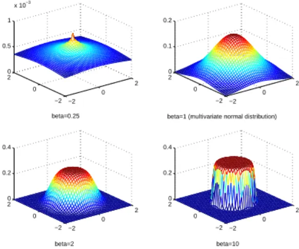
Figure 1: Matrix PE density function withn= 1,p= 2,Φ =I1,Σ =I2and variateβ.
Letk(i) denote thep-dimensional vector whoseith entry is 1 and all the others are 0. Letl(i) denote the n-dimensional vector whoseith entry is 1 and all the others are 0. SinceZ is non-degenerate, it must have an elementzi0j0 which is non-degenerate. Sincezi0j0 = l0(i0)Zk(j0),
from Theorem 4 of S´anchez-Manzano et al. ( [31]), there arezi0j0 ∼P E(mi0j0,1φi0i01σj0j0, β1)
andzi0j0 ∼P E(mi0j0,2φi0i02σj0j0, β2). So we haveβ2 = β1 and2φi0i02σj0j0 = 1φi0i01σj0j0.
From Gupta and Varga ( [21, p.24]), there must beΦ2⊗Σ2 = Φ1⊗Σ1. By the Theorem 1.3.16 of Gupta and Varga ( [21, p.13]), there exists a nonzero real number c such thatΣ2 = cΣ1 and
Φ2= Φ1/c. IfΦ2 = Φ1= Φ, thenc= 1andΣ2= Σ1. ¤
From the proof of Theorem 2.1, the only case that a matrix multivariate PE distribution is not uniquely defined is that there exist positive constantcsuch thatΣ2 =cΣ1andΦ2 = Φ1/c. So if the parameterΣorΦis known, then the distribution is uniquely defined by the other three param-eters. Therefore, in the rest of this paper, we only consider the case that parameterΦis known to handle the uniqueness issue.
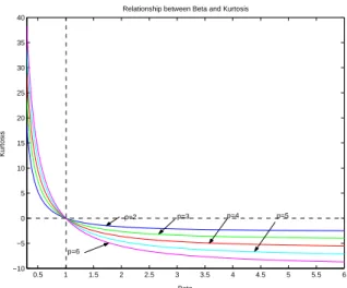
An advantage of PE distribution is that it is adaptive to bothpeakednessandflatness in the data by varying the values ofβ. Whenβincreases, the sharpness diminishes. Figure 1 represents the plot of (2.2) withn= 1,p= 2,Φ = I1,Σ = I2and the shape parameterβ. The relationship betweenβ andγ2 for the multivariate PE distribution is shown in Figure 2. Forβ = 1, (2.2) is a multivariate normal distribution and forβ → ∞, (2.2) is a multivariate uniform distribution. We note that as the dimension of the distribution gets larger, the kurtosis gets larger for bothβ < 1
0.5 1 1.5 2 2.5 3 3.5 4 4.5 5 5.5 6 −10
−5 0 5 10 15 20 25 30 35 40
Relationship between Beta and Kurtosis
Kurtosis
Beta
p=2 p=3 p=4 p=5
p=6
Figure 2: The relationship betweenβand kurtosis.
3. Type I Multivariate PE Regression Model
In model (1.1), if we assume that the rows of the random error matrixE are drawn indepen-dently fromP Ep(0,Σ, β)distribution, i.e.,ε(1), ε(2),· · · , ε(n)arei.i.d.andε(1) ∼P Ep(0,Σ, β), then y(i) ∼ P Ep(B0x
(i),Σ, β). We denote the multivariate linear regression model under this assumption as Type I MVPER model. In this case, the likelihood function is
L(B,Σ, β|Y, X) =k1exp(−12
n X
i=1
((y(i)−B0x(i))0Σ−1(y(i)−B0x(i)))β), (3.1)
where
k1 =
pnΓn(p
2)
πnp/2Γn(1 + p
2β)2
n+np2β |Σ| −n/2.
The log likelihood function is
l(B,Σ, β|Y, X)≡logL(B,Σ, β|Y, X)
=nlog(pΓ(p2))−np2 log(π)−nlog Γ(1 + 2pβ)−n(1 +p/2β) log 2
−n
2log|Σ| −12
Pn
i=1((y(i)−B0x(i))0Σ−1(y(i)−B0x(i)))β.
(3.2)
Letθ= (b0, V ec0(Σ), β)0,ε
(i)=y(i)−B0x(i)andti =ε0−(i)1ε(i). Differentiating (3.2) with respect tob,V ec(Σ)andβrespectively, we have
∂l(θ)
∂b =β
n X
i=1
tβi−1V ec(Σ−1ε(i)x0(i)), (3.3)
∂l(θ) ∂V ec(Σ) =−
n
2V ec(Σ
−1) +β
2
n X
i=1
and
∂l(θ)
∂β =
np
2β2ψ(1 +
p
2β) +
np
2β2 log 2−
1 2
n X
i=1
tβi logti, (3.5)
where ψ(·) = dlog Γ(x)/dx is called digamma function ( [1]), or psi function. To derive and construct the Fisher information matrix (FIM) and its inverse IFIM, we have
∂2(θ) ∂b0∂b =β
n X
i=1
(Ipq⊗V ec0(Ip))(Iq⊗Mi⊗Ip)(V ec(Iq)⊗Ipq), (3.6)
where
Mi=−tβi−1V ec(Σ−1)V ec0(x(i)x0(i))−2(β−1)tβi−2(Σ−1ε(i)x0(i))⊗(Σ−1ε(i)x0(i)).
∂2l(θ)
∂V ec0(Σ)∂V ec(Σ)= (Ip2⊗V ec0(Ip))(Ip⊗
∂2l(θ)
∂Σ∂Σ⊗Ip)(V ec(Ip)⊗Ip2)), (3.7)
where
∂2l(θ)
∂Σ∂Σ = n2V ec(Σ−1)V ec0−1)
−β2 Pn
i=1
tβi−1(V ec(Σ−1)V ec0−1ε (i)ε0−(i)1)
+V ec(Σ−1ε(i)ε(0−i)1)V ec0−1))
−β(β2−1) Pn
i=1
tβi−2(Σ−1ε
(i)ε0−(i)1)⊗(Σ−1ε(i)ε0−(i)1).
∂2l(θ)
∂β2 = −npβ3ψ(1 + 2pβ)− np 2
4β4ψ0(1 +2pβ)− npβ3 log 2−12
n P
i=1
tβi log2ti, (3.8)
whereψ0(·) =d2log Γ(x)/dx2 is called trigamma function.
∂2l(θ)
∂V ec0(Σ)∂b =β n X
i=1
(Ipq⊗V ec0(Ip))(Iq⊗Ni⊗Ip)(V ec(Iq)⊗Ip2), (3.9)
where
Ni= −tβi−1V ec(Σ−1)V ec0−1ε(i)x0(i))
−(β−1)tiβ−2(Σ−1ε(i)x0−(i)1ε(i)ε0−(i)1).
∂2l(θ)
∂β∂b =
n P
i=1
tβi−1V ec(Σ−1ε
(i)x0(i)) +β
n P
i=1
tβi−1log(ti)V ec(Σ−1ε(i)x0(i)). (3.10)
∂2l(θ)
∂β∂V ec(Σ) = 12
n P
i=1
tβi−1V ec(Σ−1ε (i)ε0−(i)1)
+β2 Pn
i=1
tβi−1log(ti)V ec(Σ−1ε(i)ε0−(i)1).
(3.11)
Some of the details of the above derivations are given in the Appendix. Since there are no closed form solutions to the likelihood equations, numerical methods such asGenetic Algorithms
Step 1 : ComputeBˆ = (X0X)−1X0Y.
Step 2 : Letdi =ε0(i)V ar(y(i))−1ε(i). di actually is the squaredMahalanobis distances. By the probability characteristics of multivariate PE distribution, we have
E[t2i] = 2
2/βΓ(p+4 2β )
Γ(2pβ) .
Then
E[d2i] =E[ p
2Γ2( p
2β)
22/βΓ2(p+2
2β )
t2i] = p
2Γ(p
2β)Γ(p2+4β )
Γ2(p+2
2β )
.
So we can computeβˆas the solution of
p2Γ(p
2 ˆβ)Γ( p+4
2 ˆβ )
Γ2(p+2
2 ˆβ )
= 1
n
n X
i=1
ˆ d2i
wheredˆi = (y(i)−Bˆ0x(i))0−1(y(i)−Bˆ0x(i)) andS = (Y −XBˆ)0(Y −XBˆ)/n is the sample covariance matrix.
Step 3 : Compute
ˆ
Σ = pΓ(
p
2 ˆβ)
21/βˆΓ(p+2
2 ˆβ )
S.
4. Type II Multivariate PE Regression Model
If we assume that the random error termsV ec(E0)in model (1.2) has a multivariate PE distri-butionP Enp(0,Φ⊗Σ, β), i.e.,V ec(Y0)∼P Enp((X⊗Ip)bpq×1,Φ⊗Σ, β)or with the matrix notationY ∼M P En×p(XB,Φ,Σ, β), whereΦis a(n×n)positive definite symmetric matrix and known, then the density function ofEis:
f(E; Φ,Σ, β) =k|Φ|−p/2|Σ|−n/2exp(−1
2(tr(Σ
−1E0−1E))β) (4.1)
or, the density function ofY is:
f(Y;B,Φ,Σ, β) =k|Φ|−p/2|Σ|−n/2exp(−1
2(tr(Σ
−1(Y −XB)0−1(Y −XB)))β). (4.2)
Under the assumption of Type II MVPER model, the likelihood function is:
L(B,Σ, β) =k|Φ|−p/2|Σ|−n/2exp(−1
2(tr(Σ
−1(Y −XB)0−1(Y −XB)))β), (4.3)
and the log likelihood function is:
l(B,Σ, β)≡logL(B,Σ, β)
= log(npΓ(np2 ))−np2 log(π)−log Γ(1 +np2β)−(1 +np/2β) log 2
−p2log|Φ|−n
2 log|Σ| −12(tr(Σ−1(Y −XB)0−1(Y −XB)))β.
(4.4)
Letθ=(b0, V ec0(Σ), β)0. Differentiating (4.4) with respect tob,V ec(Σ)andβ respectively, we have
∂l(θ)
∂b =V ec((
∂l(θ)
∂B )
0−1E0−1E))β−1V ec(Σ−1E0−1X), (4.5)
∂l(θ)
∂V ec(Σ) = V ec(
∂l(θ)
∂Σ )
= −n
2V ec(Σ−1) +β2(tr(Σ−1E0−1E))β−1V ec(Σ−1E0−1E)
(4.6)
and
∂l(θ)
∂β = 2npβ2ψ(1 + np2β) +2npβ2 log 2
−1
2(tr(Σ−1E0−1E))βlog(tr(Σ−1E0−1E)).
(4.7)
To derive and construct the FIM and IFIM of the model parameters, we have
∂l2(θ)
∂b0∂b = ∂∂b0(∂l∂(bθ))
= (Ipq⊗V ec0(I
p))(Iq⊗ ∂l
2(θ)
∂B0∂B0 ⊗Ip)(V ec(Iq)⊗Ipq)
(4.8)
where
∂l2(θ)
∂B0∂B0 = β(tr(Σ−1E0−1E))β−1∂(Σ
−1E0−1X)
∂B0
+(Σ−1E0−1X)⊗∂(β(tr(Σ−1E0−1E))β−1)
∂B0 ,
(4.9)
∂(Σ−1E0−1X)
∂B0 = −V ec(Σ−1)V ec0(X0−1X) (4.10) and
∂(β(tr(Σ−1E0−1E))β−1)
∂B0 =−2β(β−1)(tr(Σ−1E0−1E))β−2Σ−1E0−1X. (4.11) ∂l2(θ)
∂V ec0(Σ)∂V ec(Σ) = (Ip2 ⊗V ec0(Ip))(Ip⊗∂l 2(θ)
∂Σ∂Σ⊗Ip)(V ec(Ip)⊗Ip2) (4.12) where
∂l2(θ)
∂Σ∂Σ = n2V ec(Σ−1)V ec0−1)
−β2(tr(Σ−1E0−1E))β−1(V ec(Σ−1)V ec0−1E0−1EΣ−1)
+V ec(Σ−1E0−1EΣ−1)V ec0−1))
−β(β2−1)(tr(Σ−1E0−1E))β−2
((Σ−1E0−1EΣ−1)⊗(Σ−1E0−1EΣ−1)).
∂l2(θ)
∂β2 = −npβ3ψ(1 +np2β)−n 2p2
4β4 ψ0(1 +np2β)−npβ3 log 2
− 12(tr(Σ−1E0−1E))βlog2(tr(Σ−1E0−1E)). (4.14) ∂l2(θ)
∂β∂b = (tr(Σ
−1E0−1E))β−1V ec(Σ−1E0−1X)(1 +βlog(tr(Σ−1E0−1E))). (4.15)
∂l2(θ)
∂β∂V ec(Σ) = 12(tr(Σ−1E0−1E))β−1V ec(Σ−1E0−1EΣ−1)
(1 +βlog(tr(Σ−1E0−1E))). (4.16)
∂l2(θ)
∂V ec0(Σ)∂b = (Ipq⊗V ec0(Ip))(Iq⊗
∂l2(θ)
∂Σ∂B0 ⊗Ip)(V ec(Iq)⊗Ip2) (4.17) where
∂l2(θ)
∂Σ∂B0 = −β(tr(Σ−1E0−1E))β−1V ec(Σ−1)V ec0−1E0−1X)
−β(β−1)(tr(Σ−1E0−1E))β−2(Σ−1E0−1X)⊗(Σ−1E0−1EΣ−1). (4.18) Further details of the above derivations are given in the Appendix of the paper.
By the probability characteristics of multivariate PE distribution, we have
E[((V ec(Y0)−V ec(B0X0))0V ar(V ec(Y0−1(V ec(Y0)−V ec(B0X02]
= (np)
2Γ(np
2β)Γ(
np+4
2β )
Γ2(np+2 2β )
.v
Then, the method of moment estimate ofβ, denoted asβˆ, can be obtained by solving the equation:
((V ec(Y0)−V ec( ˆB0X0))0−1(V ec(Y0)−V ec( ˆB0X02 = (np)
2Γ(np
2 ˆβ)Γ( np+4
2 ˆβ )
Γ2(np+2
2 ˆβ ) where
S= (V ec(Y0)−V ec( ˆB0X0))(V ec(Y0)−V ec( ˆB0X0))0
and
ˆ
B = (X0X)−1X0Y
is the method of moment estimate of B. By Anderson and Fang ( [17, p.215]), the unbiased estimator ofΣcan be obtained as
ˆ
Σ = npΓ(
np
2 ˆβ)
(n−q)21/βˆΓ(np+2
2 ˆβ )
(Y −XBˆ)0−1(Y −XBˆ).
Under the assumption of Type II MVPER model, indeed the sample size is only 1. According to Gupta and Varga ( [21, p.224]), the MLEs of the model parameters do not exist without imposing some restrictions on Σand Φeven if Φis known. For n ≥ p, sinceh(t) = kexp(−tβ/2)is monotone decreasing on(0,+∞), there is
ˆ
by Theorem 7.1.1 of ( [21, p.226]) and the MLE ofΣis
ˆ
ΣM LE = p
λmax
(Y −XBˆ)0−1(Y −XBˆ)
whereλmaxis the maximum point of the function
f(λ) =λnp/2h(λ)
by Theorem 7.1.3 of ( [21, p.235]). It is easy now to show that
λmax = (ˆnp
βM LE)
1/βˆM LE
by the Lemma 2 of ( [17, p.204]). However, if we substitute ΣˆM LE and BˆM LE into the log likelihood function (4.4), the log likelihood function ofβbecomes:
f(β) = log(npΓ(np2 ))− np2 log(π)−log Γ(1 +np2β)−log 2−np2 logp−p2log|Φ|
−n2 log|(Y −XBˆ)0−1(Y −XBˆ)|+np2β log(np2β)−np2β
which actually has no maximum.
We get around this problem by providing two methods to compute the MLEs of Type II MVPER model parameters. One method is to maximize the log likelihood function directly with an algorithm such as the GA given in Bozdogan and Liu ( [23]). The other method is to employ a two step procedure given as follows:
Step 1 : Use a set ofmpairs of observations randomly selected from the original data to compute
ˆ
BM LE andΣˆM LE by considering the shape parameterβfixed.
Step 2 : SubstituteBˆM LE andΣˆM LE obtained inStep 1and the original sample data into the log likelihood function (4.4), thenβˆM LE is the value ofβ which maximizes the log likelihood function ofβ.
5. Information Criteria for Multivariate PE Regression Models
For a general multivariate linear or nonlinear model,AIC is defined as:
AIC =−2 logL( ˆθ) + 2k (5.1)
where k is the number of free parameters estimated within the model. So for Type I MVPER model, we have
AICModel I = −2nlog(pΓ(p2)Γ(1 + 2 ˆpβ)) +nplog(π) + 2n(1 +p/2 ˆβ) log 2
+nlog|Σˆ|+Pni=1((y(i)−Bˆ0x(i))0Σˆ−1(y(i)−Bˆ0x(i)))βˆ
+2pq+p(p+ 1) + 2
(5.2)
and for Type II MVPER model, we have
AICModel II
= −2 log(npΓ(np2 )) +nplog(π) + 2 log Γ(1 + np
2 ˆβ) + (2 +np/βˆ) log 2
+plog|Φ|+nlog|Σˆ|+ (tr( ˆΣ−1(Y −XBˆ)0−1(Y −XBˆ)))βˆ
+2pq+p(p+ 1) + 2.
(5.3)
The definition of ICOMP(IFIM) uses the concept of maximal covariance complexity which is defined as:
Definition 5.1A maximal information theoretic measure of complexity of a covariance matrix
Σof a multivariate normal distribution is
C1( Σ)≡ maxTC0(Σ)
= p2log(tr(pΣ))−12log|Σ|, (5.4)
where the maximum is taken over the orthonormal transformation T of the overall coordinate systemx1, x2,· · · , xp.
For more details on (5.4), we refer the readers to ( [9,13,14]). For a multivariate normal linear or nonlinear structural model, we define the general form of ICOMP(IFIM) as
ICOM P(IF IM) =−2 logL(ˆθ) + 2C1( ˆF−1(ˆθ)), (5.5)
where C1 denotes the maximal information-theoretic complexity of Fˆ−1, the estimated IFIM given in (5.4), and θˆis the MLE vector. So, for Type I MVPER model, we have
ICOM(IFIM)Model I
= −2nlog(pΓ(p2)Γ(1 + p
2 ˆβ)) +nplog(π) + 2n(1 +p/2 ˆβ) log +nlog 2|Σˆ|
+Pni=1((y(i)−Bˆ0x(i))0Σˆ−1(y
(i)−Bˆ 0
x(i)))βˆ+ 2C
1( ˆF−1( ˆθ)M odel I)
(5.6)
and for Type II MVPER model, we have
ICOM(IFIM)Model II
= −2 log(npΓ(np2 )) +nplog(π) + 2 log Γ(1 + np
2 ˆβ) + (2 +np/βˆ) log 2
+plog|Φ|+nlog|Σˆ|+ (tr( ˆΣ−1(Y −XBˆ)0−1(Y −XBˆ)))βˆ
+2C1( ˆF−1( ˆθ)M odel II).
The estimated observed inverse Fisher Information matrices for Type I and Type II MVPER mod-els, Fˆ−1(ˆθ)
M odel I andFˆ−1(ˆθ)M odel II, can be computed from the results of Sections 3 and 4 accordingly by
ˆ
F−1(ˆθ) =−
∂l2(θ)
∂b0∂b ∂l
2(θ)
∂V ec0(Σ)∂b ∂l
2(θ)
∂β∂b
∂l2(θ)
∂b0∂V ec(Σ) ∂l
2(θ)
∂V ec0(Σ)∂V ec(Σ) ∂l
2(θ)
∂β∂V ec(Σ)
∂l2(θ)
∂b0∂β ∂l
2(θ)
∂V ec0(Σ)∂β ∂l
2(θ)
∂β2
ˆ
θ
.
Note that the expected Fisher information matrix and its inverse for the Type I and Type II MVPER models involve complicated forms of expected values that is difficult to compute. There-fore, in what follows, it suffices for us to use the complexity of the estimated observed inverse-Fisher Information matrix (IFIM) above in our numerical examples.
6. Genetic Algorithms (GAs)
In this section to be complete and for the benefit of the general readership of the paper, we give the general background and the working of the Genetic Algorithms (GAs) for estimating model parameters and model selection contemporaneously.
Genetic Algorithm (GA) (see, e.g., Goldberg ( [19]), Holland ( [22]), Mitchell ( [27])) is a randomized, population-based heuristic optimization technique that belong to the general class of Evolutionary algorithms (EAs). GA has significant advantages such that it is independent from the complexity of the problem at hand, and not likely to be restricted to a local optimal solution, and it is easy to use in many difficult optimization problems.
Yang and Honavar ( [35]) use GA for the selection of a subset of attributes or features to represent the patterns to be classified with Neural network (NN). Bozdogan ( [8]) who introduced the GA in statistical model selection, uses the GA in the multiple regression model for subset selection of the best predictors for intelligent data mining under the normality assumption.
In GA, the criterion to rank solutions is often called afitness function. A set of solutions is called agenerationofpopulation. A specific solution is called anindividual in the population. GA improves solutions by generating a new generation of population on the base of current pop-ulation through a series ofGA operators, such ascrossoverandmutation. The first generation of population to start the GA process is generated as a set of “wildly’ guessed or randomly generated solutions. For the GA to evolve, a solution needs to be represented in binary string format. A binary string represents a solution and it is often called achromosome.
The individuals in the current population are used to generate the new population. There are different strategies to generate a new population. One strategy commonly used is the so-called called “natural” selecting strategy. With this strategy, the chance of an individual being selected is proportional to the ratio:
rj = ∆F itnessj/∆F itness (6.1)
with a ratio of two is twice as likely to be selected as an individual with a ratio of one. This approach is called theproportional selection. There are also other selection strategies such as the
rank order selection,and so forth.
A pair of individuals selected from the current population are used to generate a pair of new solutions, often called “offsprings”, through the GA operator crossover. Crossover mimics the process of mating. The pair of chromosomes chosen for crossover is controlled by thecrossover probability(Pc) which is an input parameter of the algorithm. Crossover point, where the binary string is broken for crossover, is picked randomly along each pair of parent chromosomes. In the algorithm, we give three choices of crossover types corresponding to different locations of crossover points. In the following, “|” represents a crossover point.
• Single point crossover
Parent A 10|001001001 ↓↑
Parent B 00|010011000
→ Offspring A 10|010011000
Offspring B 00|001001001
• Two point crossover
Parent A 10|001001|001 ↓↑
Parent B 00|010011|000
→ Offspring A 10|010011|001
Offspring B 00|001001|000
• Uniform crossover- bits are randomly switched between parents: Parent A 10001001001
↓↑
Parent B 00010011000
→ Possible offspring A 00000011001
Possible offspring B 10011001000
Mutation is another parameter or operator used in GA to realize a global search. During mutation, each bit in a binary string can change from 0 to 1, or from 1 to 0, with a user input probability called themutation probability(Pm). Hence, the searching process can jump to another area of the fitness landscape, instead of being limited in a local optimum area.
Our GA also allows theElitism rule(ER). When the Elitism rule is applied, the best solution of a generation will be copied without changes to the next generation. ERguarantees the individual with the best fitness in the current generation to survive in the next generation. In other words, the best solution is passed from one generation to the next and the survival of the fittest is achieved until the GA converges.
The outline of the GA procedures for model parameter estimation and model selection is sum-marized as follows:
Step 3: Rank each individual in the population according to the given fitness function. Step 4: Select individuals to be used to generate the new population.
Step 5: Do crossover on selected individuals with a given crossover type and crossover probabil-ity and create a new population.
Step 6: Do mutation on the new population with a given mutation probability.
Step 7: Do GA engineering on the new population with a given engineering probability.
Step 8: Do elitism if required. Elitism means that the best individual in current population is guaranteed to be included in the new population.
Step 9: Replace the current population with the new population.
Step 10: Repeat Steps 2-9 until a certain condition of the result is satisfied.
The GA for model parameter estimation and the GA for model selection share the shame out-line above, but with different objective functions (fitness functions) and solution representations. This reflects one of the significant advantages of GA method. Once a GA is set up, it can be expanded to solve different problems easily by only changing the fitness function and the repre-sentation of solution space. We will explain the fitness function and solution reprerepre-sentation for model parameter estimation and model selection in following sections. TheGA engineering(or
GA cloning) in Step 7 above is a new GA operator we developed to improve the evolution of the GA process. This will be explained in Section 6.4. The pseudo code of the steps of the GA outlined above is given in the Appendix.
6.1. GA for Model Parameter Estimation
We use GA to estimate the maximum likelihood estimators (MLEs) of the multivariate re-gression model parameters; the coefficients and the estimated inverse-Fisher information matrix (IFIM) of the model. We use the negative log likelihood function as the fitness function. With this choice, the best solution is the minimum fitness value.
We encode each model parameter to be estimated in a binary string of fixed length, which is given by the investigator as an input. Since the parameters are real numbers, we use the following scheme to encode them. Given a real interval[a, b]and the length of binary stringl, the binary string000· · ·000representsaand111· · ·111representsb. Adding binary1to an existing binary number increases its real value by(b−a)/2l−1. With this approach, decoding a binary string to real number is easy. For example, ifl= 5, then10010represents the real valuea+ (b−a)×18/31 =
(13a+ 18b)/31.
6.2. GA for Model Selection
In the GA for model selection, we use the ICOMP(IFIM) as the fitness function. The algorithm can also be easily edited to use other model selection criteria. We encode each model using the following scheme.
Each model, or subset, is encoded as a binary string with a fixed length based on the number of total available independent variables (including the constant term). Each bit in the string is a binary code indicating the presence (1) or absence (0) of a given predictor variable in the model. For example, if there are10predictor variables available in a given data set, then the string1010110110
represents a model, where constant term is included in the model, variable1is excluded from the model, variable2is included in the model, and so on.
6.3. GA on GA Hybridization
We combine and hybridize the GA for parameter estimation and the GA for model selection as follows:
• First, the GA for model selection is called to select the best subset of predictor variables.
• At each step a model is chosen to be evaluated. Then the GA for model parameter estimation is called to obtain the MLEs of the model parameters, or the MLEs are retrieved if the model has been evaluated before. The fitness, i.e., ICOMP(IFIM) of the model is computed using the MLEs of the model parameters.
With the GA on GA approach, the output of the GA for estimation is used in the fitness function (ICOMP) to evaluate the best subset candidate models. The estimation in fact initially acts as the fitness function of the model selection in GA.
The GA on GA approach inherits both advantages and disadvantages of the general GA. But the major convenience of the GA on GA approach is that both the estimation and model selection in GA can share the same GA procedure and code. Only the fitness functions and representations of the solutions need to be changed correspondingly.
6.4. A New GA Operator: GA Engineering
GA engineering is a new operator we developed and introduced to improve the evolution of the GA process. Since GA is a “random” or “stochastic” search method, it is not guaranteed that each run of the GA with the same settings will converge to the same optimal solution. With classic GA operators and the proper setting of the parameters, the bias and variance of MLEs caused by the GA are usually acceptable according to Chatterjee ( [15]). But for the GA on GA approach, the bias and variance caused by GA during the estimation of the model parameters will affect the GA for model selection.
For this reason, we introduce the GA engineering (or GA cloning) operator to improve the es-timation further. If the population evolves “naturally” with classic GA operators, GA engineering means to improve the quality of the population “artificially”. The idea of GA engineering comes from the fact that the difference of the fitness values between the two chromosomes is caused by the bits with different binary codes in these two chromosomes and the bit in the chromosome with better fitness are supposed to contain better genes/information. For example, given
Chromosome A 100101110
(Fitness A=10)
Chromosome B 101100101
(Fitness B=20)
→ Different bits in A t t0t t1t10
Different bits in B t t1t t0t01 ,
t t0t t1t10is supposed to have better genes thant t1t t0t01if a smaller fitness value is preferred. So, if we compare the best chromosome of generationiwith that of generationi+ 1, with probabilityPe, and find that they have different binary codes and bits, then we prefer the bits corresponding to the chromosome which has the smaller fitness value, since we are minimizing the information criteria to pick the best model. Indeed, our simulation results show that this new operator does reduce the bias and variance caused by the GA. This we like.
7. Numerical Examples 7.1. Simulation Examples
In the following simulation examples, we use the procedure described by G´omez-Villegas and S´anchez-Manzano et al. ( [20]) to generate PE random vectors. The GA on GA approach developed in Bozdogan and Liu ( [23]) is used to select predictor variables and to estimate the model parameters. Predictor variables are simulated using the following simulation protocol. The first three predictors are simulated by
x1 = 10 +ε1
x2 = 10 + 0.3ε1+αε2,whereα=
√
1−0.32 = 0.9539
x3 = 10 + 0.3ε1+ 0.5604αε2+ 0.8282αε3
(7.1)
which are simulated by:
x4 = 4×rand(0,1),· · ·,xi=i×rand(0,1) (7.2)
whererand(0,1)generates the uniform random numbers in(0,1). The response variables are generated from:
Yn×2= [1, Xn×3]B4×2+En×2 (7.3)
withX = [x1,x2,x3]and
B =
8 −5
1 0.5
0.5 0
0.3 0.3
.
The error terms in (7.3) are now multivariate PE (MPE) distributed rather than multivariate normal (MN).
7.1.1. Example 1: Model Parameter Estimation and Model Selection
In this example, we generatex1,x2,andx3from (7.1) and generateY from (7.3) with sample size
n= 500. The rows ofEarei.i.d. P E2(0,Σ, β)with
Σ =
·
1 0.5
0.5 2
¸
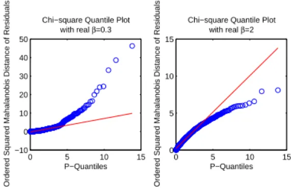
which is positive definite symmetric. We simulate two cases, β = 0.3 and β = 2 with the two dimensional plots given in Figure 1. To these simulated data sets, we fit both multivariate regression model under normality assumption and Type I MVPER model. In this case, we expect that the Type I MVPER model would be chosen as our best model according to the minimum of AIC or ICOMP, and that the model parameters would be estimated correctly, since our true model is generated under the MPE assumption. We are especially interested in the estimates ofβ. The results of200runs of both simulation cases are reported in Table 1.
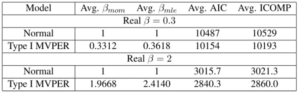
Table 1: Results of the Simulation Example 1.
Model Avg.βmom Avg.βmle Avg. AIC Avg. ICOMP Realβ= 0.3
Normal 1 1 10487 10529
Type I MVPER 0.3312 0.3618 10154 10193
Realβ = 2
Normal 1 1 3015.7 3021.3
Type I MVPER 1.9668 2.4140 2840.3 2860.0
0.1 0.2 0.3 0.4 0.5 0.6 0
10 20 30
Histogram of estimated βmom
with real β=0.3
0.1 0.2 0.3 0.4 0.5 0.6 0
10 20 30
Histogram of estimated βmle
with real β=0.3
1 1.5 2 2.5 3 0
5 10 15 20 25
Histogram of estimated βmom
with real β=2
0 2 4 6 8
0 10 20 30 40 50
Histogram of estimated βmle
with real β=2
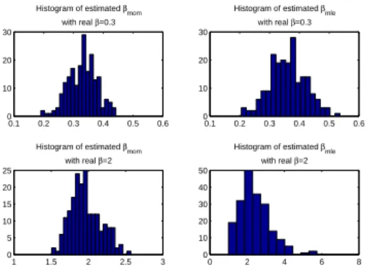
Figure 3: The MOM Estimates and MLEs ofβin 200 Runs of Simulation Example 1.
parameterβare close to the true values. The multivariate normal regression model has never been chosen by looking at the average values of AIC and ICOMP across the200runs of the simulation. The distributions of MOM estimates and MLEs ofβin the200runs of the simulation are shown in Figure 3. The Q-Q plots for the Type I MVPER model in one run of the simulation example are shown in Figure 4. From the Q-Q plots, we see that the Type I models are far from normal models for bothβ = 0.3 andβ = 2, which we expected. Figure 5 shows a typical GA process used to estimated the model parameters in one run of the simulation. The GA parameters are given in Table 2, where N Gis the number of generations,P S is the population size,Pc is the crossover probability,Pmis the mutation probability,Peis the GA engineering probability,CT is the crossover type,lis the length of the binary string used to encode real numbers, andN Ris the number of GA runs.CT = 3means uniform crossover method is used.
Table 2: GA parameters of the Simulation Example 1.
GA parameters N G P S Pc Pm Pe CT l N R Elitisim
Values 50 100 0.7 0.1 0.5 3 32 200 Yes
7.1.2. Example 2: Subset selection
In this example, we show the subset selection of the best predictors under Type I MVPER model with AIC and ICOMP(IFIM). In this simulation, three correct predictors need to be selected from total of ten available predictor variables, wherex4,· · · ,x10are considered as redundant variables. We generatex1,· · · ,x10from (7.1) and (7.2), and generateY from (7.3) with sample sizen =
500. The rows ofE arei.i.d. P E2(0,Σ, β)with
Σ =
·
1 0.5
0.5 2
¸
,
0 5 10 15 −10
0 10 20 30 40 50
Chi−square Quantile Plot with real β=0.3
Ordered Squared Mahalanobis Distance of Residuals
P−Quantiles
0 5 10 15
0 5 10 15
Chi−square Quantile Plot with real β=2
Ordered Squared Mahalanobis Distance of Residuals
P−Quantiles
Figure 4: The Q-Q plots for Type I MVPER Models in One Run of the Simulation Example 1.
0 10 20 30 40 50
1060 1080 1100 1120 1140 1160 1180 1200 1220 1240
A Typical GA Procedure in one Run of Simulation Example 1
−loglikelihood of the fitted model
GA Generations
Figure 5: A Typical GA Process in One Run of the Simulation Example 1.
3. Method of moments (MOM) estimates are used as the starting values for the GA process. For
11 independent variables (including the constant term), there are 211 = 2048possible subsets. Each subset, or model, is encoded as a binary string with the fixed length as the total number of available independent or predictor variables. Each locus in the string is a binary code indicating the presence (1) or absence (0) of a given predictor variable in the model. For example, the string
101011represents a model, where constant term is included in the model, variablex1is excluded
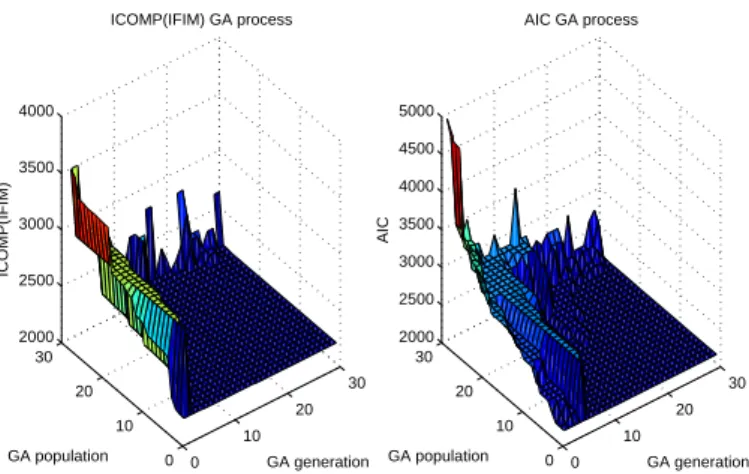
from the model, variablex2 is included in the model, and so on. Figure 6 shows the plots of all subsets evaluated in the GA process. Both GA processes converge to the true model. The top 5 subsets selected by the minimum ICOMP(IFIM) and AIC are summarized in Table 4. From Table 4, we see that the true model is selected as the best subset according to minimum ICOMP(IFIM) and AIC. The MLEs of the best model parameters chosen by ICOMP are:
ˆ
0 10
20 30
0 10 20 30 2000 2500 3000 3500 4000
GA generation ICOMP(IFIM) GA process
GA population
ICOMP(IFIM)
0 10
20 30
0 10 20 30 2000 2500 3000 3500 4000 4500 5000
GA generation AIC GA process
GA population
AIC
Figure 6: The GA Process for the Simulation Example 2 for ICOMP and AIC.
ˆ
ΣM LE =
·
0.8788 0.4007
0.4007 1.7192
¸
and
ˆ
BM LE =
7.2275 −5.4046
1.0004 0.5128
0.5142 0.0951
0.3587 0.2335
.
Our results show that the GA on GA approach with ICOMP(IFIM) or AIC as the fitness func-tion can detect the true relafunc-tionship and pick the correct models. We notice that the coefficients of the redundant variables in the top 5 best subset models selected are small, which means that these redundant variables can be ignored.
Table 3: GA parameters of the Simulation Example 2 and the Real Data Example.
N G P S Pc Pm Pe CT l Elitism
Subset GA 30 30 0.7 0.01 0.5 3 Yes
Model estimation GA 50 100 0.7 0.01 0.5 3 32 Yes
7.2. A Real Example: A Macroeconomic Time Series Data
In this last example, we use the famous quarterly macroeconomic time series data for the United Kingdom during 1948-1956. This data set consists of n = 36 quarterly observations, starting with the first quarter of 1948 and ending with the last quarter of 1956. All then = 36
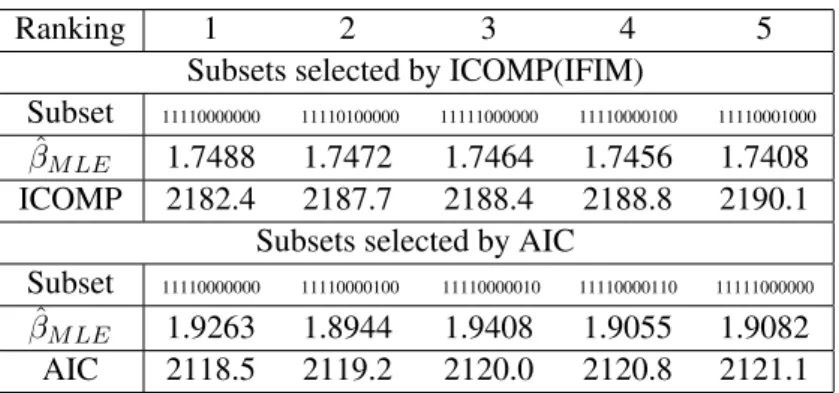
Table 4: Top 5 subsets according to minimum AIC and ICOMP(IFIM).
Ranking 1 2 3 4 5
Subsets selected by ICOMP(IFIM)
Subset 11110000000 11110100000 11111000000 11110000100 11110001000
ˆ
βM LE 1.7488 1.7472 1.7464 1.7456 1.7408
ICOMP 2182.4 2187.7 2188.4 2188.8 2190.1
Subsets selected by AIC
Subset 11110000000 11110000100 11110000010 11110000110 11111000000
ˆ
βM LE 1.9263 1.8944 1.9408 1.9055 1.9082
AIC 2118.5 2119.2 2120.0 2120.8 2121.1
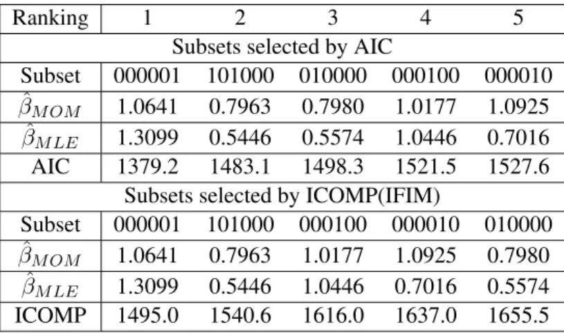
as the starting values for the GA process. AIC and ICOMP(IFIM) criteria developed in Section 5 are used for subset selection of the best predictors. The top 5 best subsets selected according to AIC and ICOMP(IFIM) scores by fitting Type I and Type II MVPER models on the Klein data set. The results are summarized in Tables 6 and 7, respectively. We can see that the results of AIC and ICOMP(IFIM) are slightly different for each type of MVPER models for this data set. For Type I MVPER model, both AIC and ICOMP(IFIM) criteria select the binary string000001as the optimal model. In other words, the predictor variablex5 =price index of consumptionis the best predictor to predict all the response variableY withβˆM LE = 1.3099which indicates that this data set is not normal.
The MLEs ofBandΣfor the optimal model are:
ˆ
BM LE,M odel I = ¡
1.0084 0.9151 0.8590 0.9793 1.0597 ¢
and
ˆ
ΣM LE,M odel I =
84.9514 9.1643 6.1158 9.5936 15.5155
9.1643 91.5875 138.4841 3.8669 −18.4478
6.1158 138.4841 576.3684 −55.7333 −54.1991
9.5936 3.8669 −55.7333 34.2577 −4.7476
15.5155 −18.4478 −54.1991 −4.7476 81.4006
.
For Type II MVPER model, both AIC and ICOMP(IFIM) select110000 as the optimal model. That is, the constant termx0 and the predictor variablex1 =total labor f orceare chosen as the best subset of predictors.
The MLEs ofBandΣfor the optimal model are
ˆ
BM LE,M odel II =
µ
−462.5338 −115.9112 473.4929 −417.9496 −505.6549
5.6339 2.1539 −3.6246 5.1773 6.0989
¶
and
ˆ
ΣMLE,M odel II =
496.1 171.4 −729.1 263.0 256.7
171.4 176.3 −188.7 25.6 26.7
−729.1 −188.7 9812.5 −1485.6 −765.4
263.0 25.6 −1485.6 973.4 275.0
256.7 26.7 −765.4 275.0 1479.4
Table 5: Variables of the Klein data set.
response variables independent variables
y1=industrial production x1 =total labor force
y2=consumption x2 =weekly wage rates
y3=unemployment x3 =price index of imports
y4=total imports x4 =price index of exports
y5=total exports x5 =price index of consumption
Table 6: Top 5 ranking subsets selected under Type I MVPER Model.
Ranking 1 2 3 4 5
Subsets selected by AIC
Subset 000001 101000 010000 000100 000010
ˆ
βM OM 1.0641 0.7963 0.7980 1.0177 1.0925
ˆ
βM LE 1.3099 0.5446 0.5574 1.0446 0.7016
AIC 1379.2 1483.1 1498.3 1521.5 1527.6
Subsets selected by ICOMP(IFIM)
Subset 000001 101000 000100 000010 010000
ˆ
βM OM 1.0641 0.7963 1.0177 1.0925 0.7980
ˆ
βM LE 1.3099 0.5446 1.0446 0.7016 0.5574 ICOMP 1495.0 1540.6 1616.0 1637.0 1655.5
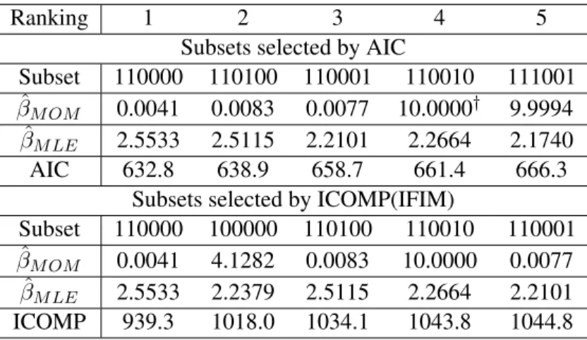
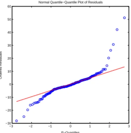
From the results in Tables 6 and 7, we see that the AIC and ICOMP(IFIM) values for the best Type II model are much smaller than those for the best Type I model. So according to the minimum value of both AIC and ICOMP(IFIM) criteria, Type II MVPER model will be selected as the best fitting model for the Klein data set. We note that such a choice is in agreement with our prior knowledge about this data set in that the observations actually are not independent. They are dependent since this data set is time dependent. We can also see that for both Type I and Type II MVPER models, the MLEs of β are different from one another, which means that the residuals are non-normal for the Klein data set. Here we use Q-Q plots to test the normality of the residuals. For the Type I model, if the residuals are i.i.d. multivariate normally distributed, the squared Mahalanobis distance of each residual vector,di = ε0−(i)1S−1ε(i), will be distributed approximately asχ2withpdegrees of freedom, wherep= 5is the number of dependent variables in the model. So the Q-Q plot for Type I model is the ordered distance values di against the corresponding theoretical quantiles ofχ2(5)distribution. For the Type II model, we first vectorize the residuals and then do the plot as the classic normal Q-Q plot. The Q-Q plots are shown in Figures 7 and 8, respectively. From the graphs, we see that the Type I model is closer to the normal model according to the estimatedβ values. However, we see that the best fitting Type II model does not follow the normal distribution based on the estimatedβ values. Indeed, this data set has serial correlations which causes the fact that the probability distribution of the model is misspecified. Type II model captures such misspecification as a general and flexible model which
†The GA is setup to searchβin [0.001 10]. If the MLE ofβis very near to 10, we consider the estimate is∞. If the
Table 7: Top 5 ranking subsets selected under Type II MVPER Model.
Ranking 1 2 3 4 5
Subsets selected by AIC
Subset 110000 110100 110001 110010 111001
ˆ
βM OM 0.0041 0.0083 0.0077 10.0000† 9.9994
ˆ
βM LE 2.5533 2.5115 2.2101 2.2664 2.1740
AIC 632.8 638.9 658.7 661.4 666.3
Subsets selected by ICOMP(IFIM)
Subset 110000 100000 110100 110010 110001
ˆ
βM OM 0.0041 4.1282 0.0083 10.0000 0.0077
ˆ
βM LE 2.5533 2.2379 2.5115 2.2664 2.2101
ICOMP 939.3 1018.0 1034.1 1043.8 1044.8
takes the dependency structure of the data into account.
0 5 10 15
0 5 10 15
Chi−square Quantile−Quantile Plot
Ordered Squared Mahalanobis Distance of Residuals
P−Quantiles
Figure 7: Q-Q plot under the Type I model.
8. Conclusion
In this paper we presented a new and novel model selection technique to deal with non-normality in multivariate regression models using information-theoretic model selection criteria such as AIC and ICOMP. We developed two types of MVPER models. These two types of MVPER models discussed in this paper can be used to model random phenomena whose observations are
−3 −2 −1 0 1 2 3 −30
−20 −10 0 10 20 30 40 50 60
Normal Quantile−Quantile Plot of Residuals
Ordered Residuals
P−Quantiles
Figure 8: Q-Q plot under the Type II model.
not be obtained from a single sample. But a two step re-sampling method is used and developed to solve this problem. Our simulated as well as the real computational examples show that the hy-brid of information criteria such as AIC and ICOMP(IFIM) and the GA approach works well for model selection in both cases. Advantages of this approach introduced in this paper are flexible to resolve many problems in vector autoregressive (VAR) models, in kernel support vector machines (SVMs), etc. by taking the dependency in the data into account.
All our computations are carried out using a newly developed computational MATLAB mod-ules with GA.
Acknowledgements
This paper is based on the results of the Ph.D. thesis of the first author under the supervision of Prof. Bozdogan. First author extends his thanks and gratitude to Prof. Bozdogan for all the help provided throughout. This paper has been presented by Prof. Bozdogan as an invited pa-per atBayes, Multivariate Analysis, and CASM Conferencein Honor of Professor S. Jim Press, Distinguished University Professor, at the University of California at Riverside, California during May 13-14, 2005. We are deeply honored to dedicate this paper to Professor Jim Press in honor of his 50 years of remarkable career and scientific contributions toBayesianandMultivariate Statis-ticson the occasion of his retirement. Professor Bozdogan gratefully acknowledges funding for his research from the Scholarly Research Grant Program (SRGP) Awards of the College of Busi-ness Administration at the University of TenBusi-nessee in Knoxville, during 2002-03 under the title