HAL Id: hal-02290310
https://hal.inria.fr/hal-02290310
Submitted on 18 Sep 2019
HAL
is a multi-disciplinary open access
archive for the deposit and dissemination of
sci-entific research documents, whether they are
pub-lished or not. The documents may come from
teaching and research institutions in France or
L’archive ouverte pluridisciplinaire
HAL
, est
destinée au dépôt et à la diffusion de documents
scientifiques de niveau recherche, publiés ou non,
émanant des établissements d’enseignement et de
recherche français ou étrangers, des laboratoires
Evaluation of Deep Species Distribution Models using
Environment and Co-occurrences
Benjamin Deneu, Maximilien Servajean, Christophe Botella, Alexis Joly
To cite this version:
Benjamin Deneu, Maximilien Servajean, Christophe Botella, Alexis Joly. Evaluation of Deep Species
Distribution Models using Environment and Co-occurrences. CLEF 2019 - Conference and Labs of
the Evaluation Forum, Sep 2019, Lugano, Switzerland. �hal-02290310�
Evaluation of Deep Species Distribution Models
using Environment and Co-occurrences
Benjamin Deneu
1, Maximilien Servajean
2, Christophe Botella
3,
and Alexis Joly
11
Inria, LIRMM, Montpellier, France, [email protected], [email protected]
2
AMIS, Universit´e Paul Val´ery Montpellier, LIRMM UMR 5506, CNRS, [email protected]
3INRA, Inria, AMAP, LIRMM, Montpellier, France, [email protected]
Abstract
This paper presents an evaluation of several approaches of plants species distribution modeling based on spatial, environmental and co-occurrences data using machine learning methods. In particular, we re-evaluate the environmental convolutional neural network model that ob-tained the best performance of the GeoLifeCLEF 2018 challenge but on a revised dataset that fixes some of the issues of the previous one. We also go deeper in the analysis of co-occurrences information by evaluating a new model that jointly takes environmental variables and co-occurrences as inputs of an end-to-end network. Results show that the environmental models are the best performing methods and that there is a significant amount of complementary information between co-occurrences and envi-ronment. Indeed, the model learned on both inputs allows a significant performance gain compared to the environmental model alone.
1
Introduction
Automatically predicting the list of species that are the most likely to be ob-served at a given location is useful for many scenarios in biodiversity informatics. First of all, it could improve species identification processes and tools by reduc-ing the list of candidate species that are observable at a given location (be they automated, semi-automated or based on classical field guides or flora). More generally, it could facilitate biodiversity inventories through the development of location-based recommendation services (typically on mobile phones) as well as the involvement of non-expert nature observers. Last but not least, it might serve educational purposes thanks to biodiversity discovery applications provid-ing innovative features such as contextualized educational pathways.
This problem is known as Species Distribution Modeling (SDM) in ecology. SDM have become increasingly important in the last few decades for the study
of biodiversity, macro ecology, community ecology and the ecology of conser-vation. An accurate knowledge of the spatial distribution of species is actually of crucial importance for many concrete scenarios including landscape man-agement, preservation of rare and/or endangered species, surveillance of alien invasive species, measurement of human impact or climate change on species, etc. Concretely, the goal of SDM is to infer the spatial distribution of a given species, and they are often based on a set of geo-localized occurrences of that species (collected by naturalists, field ecologists, nature observers, citizen sci-ences project, etc.). However, it is usually not reliable to learn that distribution directly from the spatial positions of the input occurrences. The two major problems are the limited number of occurrences and the bias of the sampling effort compared to the real underlying distribution. In a real-world dataset, the raw spatial distribution of the occurrences is actually highly influenced by the accessibility of the sites and the preferences and habits of the observers. An-other difficulty is that an occurrence means a punctual presence of the species, while no occurrences doesn’t mean the species is absent, which makes us very uncertain about regions without observed specimens.
For all these reasons, SDM is usually achieved throughenvironmental niche modelingapproaches,i.e. by predicting the distribution in the geographic space on the basis of a representation in the environmental space [1, 2, 3, 4, 5, 6, 7]. This environmental space is in most cases represented by climate data (such as temperature, and precipitation), but also by other variables such as soil type, land cover, distance to water, etc. Then, the objective is to learn a function that takes the environmental feature vector of a given location as input and outputs an estimate of the abundance of the species. The main underlying hy-pothesis is that the abundance function is related to thefundamental ecological niche of the species. That means that in theory, a given species is likely to live in a privileged ecological niche, characterized by an hypervolume in the envi-ronmental space. However, this volume can have a very irregular shape and, in addition, many phenomena can actually affect the distribution of the species relative to its so calledabioticpreferences. The real distribution of the species is calledrealized ecological nicheit can differ from thefundamental ecological niche by environmental perturbations, geographical constraints, or interactions with other living organisms (including humans) that might have encourage specimens of that species to live in a different environment. As a consequence, therealized ecological niche of a species can be much more diverse and complex than its hypothetical fundamental niche.
Very recently, SDM based on deep neural networks have started to appear [8]. These first experiments showed that they can have a good predictive power, potentially better than the models used conventionally in ecology. Actually, deep neural networks are able to learn complex nonlinear transformations in a wide variety of domains. In addition, they make it possible to learn an area of environmental representation common to a large number of species, which sta-bilizes predictions from one species to another and improves them globally [9]. Finally, spatial patterns in environmental variables often contain useful infor-mation for species distribution but are generally not considered in conventional
models. Conversely, convolutional neural networks effectively use this informa-tion and improve predicinforma-tion performance.
In this paper, we report an evaluation study of four main kinds of plants SDM:
1. A convolutional neural network aimed at learning the ecological prefer-ences of species thanks to environmental image patches provided as inputs (temperature, soil type, etc.).
2. Two purely spatial models, one based on a random forest fitted on the spatial coordinates of the occurrences of each species. The other named closest-locations classifier is close to a nearest neighbours classifier. 3. A species co-occurrence model aiming at predicting the likelihood of
pres-ence of a given species thanks to the knowledge of the prespres-ence of other species.
4. We finally introduce a new neural network that jointly learn on environ-ment and co-occurrences and compare it to the two separated models to study the joint information between the environment and co-occurrences. And in parallel to it, a model consisting of a late merging of the outputs of the co-occurrences model and the environmental CNN.
This paper is an extended and revised version of the working note that we wrote beforehand in the context of our participation to the GeoLifeCLEF 2018 chal-lenge [10]. It improves it two main ways. First we re-evaluate the environmental convolutional neural network models that obtained the best performance during the GeoLifeCLEF 2018 challenge but on a revised dataset that fixes some of the issues of the previous one (that were discovered after the end of the challenge). We also go deeper in the analysis of co-occurrences information by evaluating a new model that jointly takes environmental variables and co-occurrences as inputs of an end-to-end network. Section 2 gives an overview of the data and evaluation methodology. Section 3 and 4 provide the detailed description of the evaluated models. Section 5 presents the results of the experiments and their analysis.
2
Data and Evaluation Methodology
A detailed description of the protocol used to build the GeoLifeCLEF2018 dataset is provided in [11, 12]. In a nutshell, the dataset was built from occur-rence data of the Global Biodiversity Information Facility (GBIF), the world’s largest open data infrastructure in this domain, funded by governments. It is composed of 291,392 occurrences of N = 3,336 plant species observed on the French territory between 1835 and 2017. This dataset was split in 3/4 for training and 1/4 for testing with the constraints that: (i) for each species in the test set, there is at least one observation of it in the train set and (ii), an
observation of a species in the test set is distant of more than 100 meters from all observations of this species in the train set.
Concerning the environmental images used to learn CNN models, those given during the 2018 session of the challenge were found to be erroneous and enabled the models to actually overfit a part of the test set (mostly the occurrences that overlapped the sea). To resolve this problem, new environmental images of each occurrence were extracted using the patch extractor from GeoLifeCLEF2019
1. The environmental data is composed of 33 environmental rasters. Each
raster encodes an environmental variable on the French territory. They were constructed from various open datasets including Chelsea Climate, ESDB soil pedology data, Corine Land Cover 2012 soil occupation data, CGIAR-CSI evap-otranspiration data, USGS Elevation data (Data available from the U.S. Geo-logical Survey.) and BD Carthage hydrologic data. To construct the input tensor we extract for each occurrence a matrix of 64×64 pixels from each raster centered of the location of the occurrence. Most of the environmental variables are continuous variables such as the average temperature, the altitude or the distance to water. Thus, the corresponding 64×64 pixel matrices can be pro-cessed as classical image channels provided as input of the CNN. Some of the variables are rather of ordinal type (such as ESDB v2). However, they still can be considered as additional channels of the CNN in the sense that the order of the pixel values remains meaningful. This is not true, however, for categorical variables such as the Corine Land Cover variable. This variable take up to 45 different categorical values but the order of these values does not have any meaning. Consequently, this patch is unstacked into 45 different binary patches. We finally obtain a tensor of size 64×64×(32 + 45 = 77) for each occurrence. In the following, we usually denote asx∈X a particular occurrence, each
xbeing associated to a spatial positionp(x) in the spatial domainD, a species label y(x) and an environmental tensorg(x) of size 64×64×77. We denote as P the set of all spatial positions p covered by X. It is important to note that a given spatial positionp∈ P usually corresponds to several occurrences
xj ∈X, p(xj) =pobserved at that location (18 000 spatial locations over a total
of 60 000, because of quantized GPS coordinates or Names-to-GPS transforms). In the training set, up to several hundreds of occurrences can be located at the same place (be they of the same species or not). The occurrences in the test set might also occur at identical locations but, by construction, the occurrence of a given species does never occur at a location closer than 100 meters from the occurrences of the same species in the training set.
The used evaluation metric is the Mean Reciprocal Rank (MRR). The MRR is a statistic measure for evaluating any process that produces a list of possible responses ordered by probability of correctness. It is well adapted to assess the scenario targeted by the GeoLifeCLEF challenge,i.e. providing a short-list of species that are the most likely to be observed at a given location to users of field applications. The reciprocal rank of a query response is the multiplicative inverse of the rank of the first correct answer. The MRR is the average of the
reciprocal ranks for the whole test set: M RR= 1 Q Q X q=1 1 rankq (1)
whereQis the total number of query occurrencesxq in the test set and rankq
is the rank of the correct speciesy(xq) in the ranked list of species predicted by
the evaluated method forxq.
3
Evaluated SDM Models in GeoLifeCLEF2018
3.1
Convolutional Neural Network
It has been previously shown in [8] that Convolutional Neural Networks (CNN) may reach better predictive performance than classical models used in ecology. Our approach builds upon this idea but differs from the one of Botellaet al in two important points:
• Softmax loss: whereas the CNN of Botellaet al. [8] was aimed at pre-dicting species abundances thanks to a Poisson regression on the learned environmental features, our model rather attempts to predict the most likely species to be observed according to the learned environmental fea-tures. In practice, this is simply done by using a softmax layer and a categorical loss instead of the Poisson loss layer used in [8].
• Model architecture: we also used a different architecture of the con-volutional layers compared to the one of Botellaet al. and the one sub-mitted during our participation in the challenge [10]. We used the incep-tion v3 architecture [13] but with the three following modificaincep-tions: (i) we change the classifier size to 3336 (number of classes), (ii) we add a dropout layer between the last fully-connected layer and the classifier, and (iii), we change the input size from 3 channels (classical images classification) to 77 channels according to the size of the input environmental tensors.
Learning set up and parameters: All our experiments were conducted using PyTorch deep learning framework2 and were run on a single computing node
equipped with 4 Nvidia GTX 1080 ti GPU. We used the Stochastic Gradient Descent optimization algorithm with a learning rate of 0.1 (divided by 10 at epoch 90, 130, 150 and 170), a momentum of 0.9, a mini-batch size of 128 and a dropout of 0.7. We perform a validation every 10 epochs and the final model is chosen as the one with the highest validation score.
3.2
Spatial Models
For this category of models, we rely solely on the spatial positionsp(x) to model the species distribution (i.e. we do not use the environmental information at all). We did evaluate two different classifiers based on such spatial data:
1. Closest-location classifier: For any occurrence xq in the test set and
its associated spatial position p(xq), we return the labels of the species
observed at the closest locationpN N inPtrain(exceptp(xq) itself ifp(xq)∈ Ptrain). The species are then ranked by their frequency of appearance
at location pN N. Note that p(xq) is excluded from the set of potential
closest locations because of the construction protocol of the test. Indeed, as mentioned earlier, it was enforced that the occurrence of a given species in the test set does never occur at a location closer than 100 meters from the occurrences of the same species in the training set. As a consequence, if we took pN N = p(xq), the right species would never belong to the
predicted set of species.
One of the problem of the above method is that it returns only a subset of species for a given query occurrencexq (i.e. the ones located at pN N.
Returning a ranked list of all species in the training set would be more profitable with regard to the used evaluation metric (Mean Reciprocal Rank). Thus, to improve the overall performance, we extended the list of the closest species by the list of the most frequent species in the training set (up to reaching the authorized number of 100 predictions for each test item).
2. Random forest classifier: Random forests are known to provide good performance on a large variety of tasks, including in ecology [14, 15], and are likely to outperform the naive closest-location based classifier described above. In particular we used the random forest algorithm implemented within the scikit-learn framework3. We used only the spatial positions
p(x) as input variables and the species labels y(x) as targets. For any occurrencexq in the test set, the random forest classifier predicts a ranked
list of the most likely species according to p(xq). Concerning the
hyper-parametrization of the method, we conducted a few validation tests on the training data and finally used 50 trees of depth 8 for the final runs submitted to the GeoLifeCLEF challenge.
3.3
Co-occurrence Model
Species co-occurrence is an important information in that it may capture inter-dependencies between species that are not explained by the observed environ-ment. For instance, some species live in a community because they share pref-erences for a kind of environment that we do not observe (communities of weeds are often specialized to fine scale agronomic practices that are not reported in our environmental data), they use the available resources in a complementary
way, or they favor one another by affecting the local environment (leguminous and graminaceous plants in permanent grasslands). On the opposite, some species are not likely to be observed jointly because they live in different envi-ronments, they compete for resources or negatively affect the environment for others (allelopathy, etc.).
To capture this co-occurrence information, it is required to train a model aimed at predicting the likelihood of presence of a given species thanks to the knowledge of the presence of other species (without using the environmental information or the explicit spatial positions). Therefore, we did train a feed-forward neural network taking species abundance vectors as input data and species labels as targets. The abundance vectors were built in a similar way than the closest-location classifier described in section 3.2. For any spatial posi-tionq∈D, we first aggregate all the occurrences located at the closest location
pN N in Ptrain (except q itself). Then, we count the number of occurrences
of each species in the aggregated set. More formally, we define the abundance vector z(q)∈RN of any spatial positionq∈Das:
∀i,∀x, zi(q) =
X
p(x)=pN N
1(y(x) =i) (2)
where1() is an indicator function equals to 1 if the condition in parenthesis is true and 0 otherwise andzi(q) is the component of z(q) corresponding to the
abundance of thei-th species at positionq.
Architecture description: The neural network we used to predict the most likely species based on a given abundance vector is a simple Multi-Layered Per-ceptron (MLP) with one hidden layer of 256 fully connected neurons. We used ReLU activation functions [16] and Batch Normalization [17] for the hidden layer, and a softmax loss function as output of the network.
Learning set up and parameters: This model was implemented and trained within PyTorch deep learning framework4 and were run on a single computing
node equipped with 4 Nvidia GTX 1080 ti GPU. We used the Stochastic Gradi-ent DescGradi-ent optimization algorithm with a learning rate of 0.001, a momGradi-entum of 0.9, a mini-batch size of 32. We perform a validation every epochs and the final model is chosen as the one with the highest validation score.
3.4
Late Fusion of Previous Models
We also produced an other model corresponding to a late fusion of the environ-mental CNN and the co-occurrence model. Indeed, the two base models being trained on different kinds of input data, we expect that their fusion may ben-efit from their complementarity. We process the late fusion by averaging the prediction probabilities of the two models and then we re-sort the predictions.
4
4
New Model using Jointly Environment and
Co-occurrences in an End-to-End Network
The previous neural networks allow to capture in one case information contained in plant co-occurrences and in the other case environmental information from patches. However, co-occurrences can also be seen as a complementary envi-ronmental information. Indeed, the species close to a plant are directly part of its environment. Thus, species interact with each other and with the physical environment. To capture the interdependencies between co-occurrences and the environment we have developed a model that uses both inputs: environmental tensors and vector of co-occurrences.
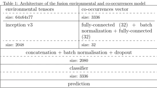
Architecture description: the environmental tensors are exactly the same as the CNN model and are described in section 2. The co-occurrences inputs remains the same as the co-occurrences model of the previous section,i.e. the abundance vector describe in section 3.3. This model is a deep neural network that is partly convolutional. The architecture is describe in table 1. It is first composed of two separate branches. One branch of the network is identical to the environmental CNN with the inception v3 architecture without the dropout layer. The other branch of the network is a small neural network like the co-occurrence model consisting in two fully-connected layer of size 32 with a batch normalization after the first one. Instead of making two classifiers, the tensors from the last layers of the two branches are concatenated and, followed by a batch normalization and a dropout layer, and finally a single classifier on this fi-nal tensor. The role of this additiofi-nal layer is to learn a common representation space that captures the potential interdependencies between the environment and the co-occurrences.
Learning set up and parameters: This model is learned with the same setup, parameters and process than the environmental CNN (see section 3.1) but with dropout of 0.8 instead of 0.7.
5
Experiments and Results
5.1
Evaluated Models Synthesis
In summary, we evaluate the six following models:
Spa-CC: the spatial closest-location classifier model (see section 3.2).
Spa-RF: the spatial random forest classifier (see section 3.2).
Cooc-NN: the co-occurrence model (see section 3.3).
Env-CNN: the environmental CNN (see section 3.1).
Env-Cooc-LF: late fusion of the probabilities given by theEnv-CNNand the
Cooc-NNmodels (see section 3.4).
Env-Cooc-JNN: joint neural network on environment and co-occurrences (see section 4).
Table 1: Architecture of the fusion environmental and co-occurrences model
environmental tensors
co-occurrences vector
size: 64x64x77 size: 3336
inception v3
fully-connected (32) + batch
normalization + fully-connected
(32)
size: 2048 size: 32
concatenation + batch normalisation + dropout
size: 2080
classifier
size: 3336
prediction
The 3 first ones (Spa-CC, Spa-RFand Cooc-NN) are exactly the same than submitted in our participation in the challenge (seeFLO 1, FLO 4and
FLO 2 in [10]). Env-CNN is the new CNN architecture (see section 3.1) that was trained on the revised GeoLifeCLEF patches. Env-Cooc-LF is the same fusion model thanFLO 5 in [10] but with the new environmental CNN predictions. Finally, Env-Cooc-JNN is our new model no submitted in our participation.
5.2
Model Selection and Validation Experiments
We conducted a first set of experiments to evaluate the performances of our models in the case of an independently and identically distributed validation set. Therefore, we extracted a part of the training set (10% occurrences selected at random) and used it as a validation set. For neural networks we extracted an additional 10% of remaining train occurrences to have a pre-validation set. We choose two cross-validation protocols :
• For the three neural network models (i.e. co-occurrences neural network, environmental CNN and environmental and co-occurrences fusion model) we choose to fix the split between training set, validation set and pre-validation set (Holdout cross-pre-validation). As, the neural networks took around one day to be learned completely, it was not workable to repeat split and learning many times. Thus, we worked with a single validation set to calibrate all our neural networks models. By fixing the split we assume to introduce a bias, but this bias is then constant between the
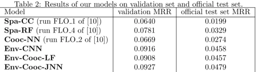
Table 2: Results of our models on validation set and official test set. Model validation MRR official test set MRR
Spa-CC(run FLO 1 of [10]) 0.0640 0.0199
Spa-RF(run FLO 4 of [10]) 0.0781 0.0329
Cooc-NN(run FLO 2 of [10]) 0.0669 0.0274
Env-CNN 0.0916 0.0458
Env-Cooc-LF 0.0908 0.0457
Env-Cooc-JNN 0.0927 0.0479
experiments which allows us to compare the performance obtained on a single learning.
• For the two spatial models, that require a lower computation time, we choose to not fix the train-validation split but to learn the model on twenty random train-validation splits (Monte Carlo cross-validation). The per-formance of a model is defined by the average perper-formance of the model on the twenty different splits. Like this we don’t introduce a bias as for the neural networks but we keep the possibility to compare two models. Note that for the random forest classifier of scikit-learn we need to have at least one occurrence of each species in the training set and one occurrence of each species in the test set. However, some species are present only once in the data, so we had to remove them for validation experiments of this model.
5.3
Results
The performance of each model is given in tables 2. In validation, the best models are those based on environmental and co-occurrences data. The Env-CNN achieves a pretty good MRR of 0.0916 knowing that the ideal MRR cannot exceed 0.409 (due to the fact that several outputs exist for the same entry). On average, it returns the correct species in the first position with a success rate of 1/30 (0.0330) (knowing that there is 3336 species in the training set). Concerning the two fusion models, if the late fusion did not result in a performance gain, the joint model (Env-Cooc-JNN) give a better score than the environmental model alone (0.0927 vs. 0.0916) and is the best model evaluated here.
Nevertheless, the other models achieve good results too, all are over 0.06 of MRR and the random forest (Spa-RF) reaches almost 0.08. They return the good species label between 1 time out of 40 and 1 time out of 30. These results show that some fairly simple models can capture a strong information. For all models, the score on the official GeoLifeCLEF 2018 test set is much lower than the one obtained in validation. However, the order of performance of the models is maintained. TheEnv-Cooc-JNNmodel remains the best on the official test set, not far but significantly ahead of theEnv-CNN model alone (0.0479 vs. 0.0458).
These results allow us to draw the following conclusions:
• official test set results vs. validation test set results: overall, the MRR values achieved by our models on the blind test set of GeoLifeCLEF are much lower than the ones obtained within our validation experiments (see Table 2). We believe that this performance loss is mainly due to the construction of the blind test set,i.e. to the fact that the occurrence of a given species in the test set does never occur at a location closer than 100 meters from the occurrences of the same species in the training set. This rule was not taken into account during our cross-validation experiments on the training set. An other point is that, for the official evaluation, the prediction size is limited at 100 ranked species for each test occurrences. We observe that this have also an impact on the MRR score.
• Supremacy of environmental models: the results show that our mod-els based on environmental data are the best performing ones. The en-vironmental CNN model (Env-CNN) is ahead from co-occurrences and spatial models. The late fusion model on environment and co-occurrences (Env-Cooc-LF) obtained similar scores to theEnv-CNNalone and the
Env-Cooc-JNNoutperform all other models on the two evaluation pro-cess. After the environmental models the spatial classifier based on ran-dom forest (Spa-RF) obtains a very fair performance considering that it only uses the spatial positions of the occurrences (which makes it very easy to implement in a real-world system). The co-occurrence model ( Cooc-NN) obtains significantly lower performance, while the closest-location classifier, which uses only the nearest point species data, is the worst model (Spa-CC).
• The new environmental and co-occurrences model: the joint envi-ronmental and co-occurrences model (Env-Cooc-JNN) is the best per-forming one. It allows a significant gain compared to the environmental model alone. This result indicates that there is a complementary informa-tion between co-occurrences and the environment. It also indicates that taking into account co-occurrences makes it possible to better characterize the ecological niche of the species compared to abiotic-only models.
• Score with new patches vs. old patches: as discussed in section 2, in this paper, we used a new set of environmental patches since a part of them was corrupted in the initial GeoLifeCLEF 2018 dataset. However, the results of this new study are still in accordance from the one reported in the context of the challenge ([10]). In particular, the performance achieved by the environmental CNN on the new dataset confirms its superior predictive power over other proposed methods during the challenge. After patch correction, it remains the best model of the challenge, even better than the model learned on old environmental patches with a score of 0.0458 against 0.0435 (seeFLO 3in [10]).
• Species community: the co-occurrence model (Cooc-NN) seems to generalize better than the closest-location classifier (Spa-CC), though both methods used almost the same input information which is the species of the neighborhood. It is likely that the neural network detect the sig-nature of a community from its input co-occurrences. For example, the network is able to predict a common Mediterranean species when it gets a rare Mediterranean species as entry. Indeed, the probability of observing this same rare species near its known observation is very small, but the closest location classifier would do the error.
• Non-performing late fusion: the late fusion between the environmen-tal model and the co-occurrence model (Env-Cooc-LF) did not result in a performance gain. However the Env-Cooc-JNN shows that there is some complementary information between co-occurrences and environ-ment. This information seems to be therefore at the intersection of the environment and co-occurrences and requires joint learning to be effec-tively captured.
6
Conclusion and Perspectives
This paper compared four main types of models aimed at predicting species dis-tribution: (i) a convolutional neural network trained on environmental variables extracted around the location of interest, (ii) a purely spatial model trained with a random forest, (iii) a co-occurrence based model aimed at predicting the like-lihood of presence of a given species thanks to the knowledge of the presence of other species, and (iv), two fusions models between the environmental CNN and the co-occurrences model, one late fusion of predictions and one learned jointly on the to inputs. Our study shows that the convolutional neural network model maintains a high score with unbiased environmental patches. Indeed, it achieved the best performance over the others GeoLifeCLEF 2018 submitted models. However the main contribution of our study is the new joint model on environment and co-occurrences that achieve good results, significantly better than the environmental CNN. This shows that there is useful information in co-occurrences and that this information is at least partly complementary to environmental information. Few studies currently use this co-occurrences in-formation. It would be interesting, in future work, to study more about how useful is the information in co-occurrences and how its complementarity with the environment can be explained.
References
[1] Antoine Guisan and Niklaus E. Zimmermann. Predictive habitat distribu-tion models in ecology. Ecological Modelling, 135(2):147 – 186, 2000.
[2] Guisan Antoine and Thuiller Wilfried. Predicting species distribution: of-fering more than simple habitat models. Ecology Letters, 8(9):993–1009, 2005.
[3] Ara´ujo Miguel B. and Guisan Antoine. Five (or so) challenges for species distribution modelling. Journal of Biogeography, 33(10):1677–1688, 2006. [4] Jane Elith, Catherine H. Graham, Robert P. Anderson, Miroslav Dud´ık,
Simon Ferrier, Antoine Guisan, Robert J. Hijmans, Falk Huettmann, John R. Leathwick, Anthony Lehmann, Jin Li, Lucia G. Lohmann, Bette A. Loiselle, Glenn Manion, Craig Moritz, Miguel Nakamura, Yoshi-nori Nakazawa, Jacob McC. Overton, A. Townsend Peterson, Steven J. Phillips, Karen Richardson, Ricardo Scachetti-Pereira, Robert E. Schapire, Jorge Sober´on, Stephen Williams, Mary S. Wisz, Niklaus E. Zimmermann, and Miguel Araujo. Novel methods improve prediction of species’ distribu-tions from occurrence data. Ecography, 29(2):129–151, 2006.
[5] Janet Franklin. Mapping species distributions: spatial inference and pre-diction. Cambridge University Press, 2010.
[6] A. Townsend Peterson. Ecological niches and geographic distributions. Princeton University Press, 2011.
[7] Alessandro Ferrarini, Mohammed H. S. A. Alsafran, Junhu Dai, and Juha M. Alatalo. Improving niche projections of plant species under cli-mate change: Silene acaulis on the british isles as a case study. Climate Dynamics, 52(3):1413–1423, Feb 2019.
[8] Pierre Bonnet Pascal Monestiez Christophe Botella, Alexis Joly and Fran¸cois Munoz. A deep learning approach to species distribution mod-elling. Multimedia Technologies for Environmental & Biodiversity Infor-matics, 2018.
[9] Laura J. Pollock, Reid Tingley, William K. Morris, Nick Golding, Robert B. O’Hara, Kirsten M. Parris, Peter A. Vesk, and Michael A. McCarthy. Understanding co-occurrence by modelling species simultaneously with a joint species distribution model (jsdm). Methods in Ecology and Evolution, 5(5):397–406, 2014.
[10] Benjamin Deneu, Maximilien Servajean, Christophe Botella, and Alexis Joly. Location-based species recommendation using co-occurrences and environment- geolifeclef 2018 challenge. InCLEF working notes 2018, 2018. [11] Christophe Botella, Pierre Bonnet, and Alexis Joly. Overview of geolifeclef 2018: location-based species recommendation. In CLEF working notes 2018, 2018.
[12] Joly, Alexis and Go¨eau, Herv´e and Botella, Christophe, Glotin, Herv´e and Bonnet, Pierre and Planqu´e, Robert and Vellinga, Willem-Pier and M¨uller,
Henning. Overview of lifeclef 2018: a large-scale evaluation of species iden-tification and recommendation algorithms in the era of ai. In Proceedings of CLEF 2018, 2018.
[13] Christian Szegedy, Vincent Vanhoucke, Sergey Ioffe, Jonathon Shlens, and Zbigniew Wojna. Rethinking the inception architecture for computer vision. CoRR, abs/1512.00567, 2015.
[14] D. Richard Cutler, Thomas C. Edwards Jr., Karen H. Beard, Adele Cutler, Kyle T. Hess, Jacob Gibson, and Joshua J. Lawler. Random forests for classification in ecology. Ecology, 88(11):2783–2792, 2007.
[15] Sacha Gobeyn, Ans M. Mouton, Anna F. Cord, Andrea Kaim, Martin Volk, and Peter L.M. Goethals. Evolutionary algorithms for species distri-bution modelling: A review in the context of machine learning. Ecological Modelling, 392:179 – 195, 2019.
[16] Vinod Nair and Geoffrey E Hinton. Rectified linear units improve restricted boltzmann machines. In Proceedings of the 27th international conference on machine learning (ICML-10), pages 807–814, 2010.
[17] Sergey Ioffe and Christian Szegedy. Batch normalization: Accelerating deep network training by reducing internal covariate shift. InInternational Conference on Machine Learning, pages 448–456, 2015.