Knowledge Discovery through Mobility Data Integration

(1)

Universit`a degli Studi di Pisa

Dipartimento di Informatica

Dottorato di Ricerca in Informatica

Ph.D. Thesis

Knowledge Discovery through Mobility

Data Integration

Paolo Cintia

Supervisor

Prof. Mirco Nanni

Supervisor

(2)

(3)

Giovane e ingenuo persi la testa, sian stati i libri o il mio provincialismo... (F. Guccini)

(4)

(5)

Acknowledgments

A popular statement says: better lucky than rich. I totally agree. At a certain point of my life, I did not know exactly what to do. Instead of asking Why dont you get a job?, Anna asked me: why dont you get a Phd?. I blamed her, at the beginning. But now I have to admit that such question made my life better. This Phd has been an amazing journey towards a sort of dreamland: I traveled all around the world, I had the chance to write a paper with one of my preferred novelist, I met plenty of wonderful people. I would like to thank everyone who made this possible. Mirco, Dino and Fosca who followed and lead me in this thesis work. Giulia, who make easier for me a lot of hard things (while making harder the easy ones). My family, whom supported every crazy idea I had in my life, Phd included. The fantastic colleagues I met here: Luca, Lorenzo, Salvo, Roberto, Giulio, Francesca, Letizia, Riccardo, Chiara, Barbara. (If you are wondering about the ordering: the key is craziness). It has been a great pleasure to work with you all.

(6)

(7)

Abstract

In the era of Big Data a huge amount of information are available from every sin-gle citizen of our hyper-connected world. A simple smartphone can collect data with different kinds of information: a big part of these are related to mobility. A smartphone is connected to networks, such as GSM, GPS, Internet (and then social networks): each of them can provide us information about where, how and why the user is moving across space and time. Data integration has a key role in this understanding process: the combination of different data sources increases the value of the extracted knowledge, even though such integration task is often not trivial. This thesis aim to represent a step toward a reliable Mobility Analysis framework, capable to exploit the richness of the spatio-temporal data nowadays available. The work done is an exploration of meaningful open challenges, from an efficient Map Matching of low sampling GPS data to Inferring Human Activities from GPS tracks. A further experimentation has been performed over GSM and Twitter data, in order to detect and recognize significant events in terms of people presence and related tweets. Another promising perspective is the use of such extracted knowledge to enrich actual geospatial Datasets with a ’Wisdom of the crowd’ dimension to derive, for instance, routing policies over road networks: most chosen paths among usual drivers are more meaningful than simple shortest paths.

(8)

(9)

Introduction

In the world of Big Data, mobility is one of the most interesting phenomena to study, both for technological and philosophical reasons. Human beings base their life on moving from a place to another one to satisfy their needs. This era of Data provides a new, giant, tool: a global microscope to observe how people move across time and space and, thus, how they live. Mobility is in fact one of the main aspect of our life. An average estimation on hours spent driving [51] is about 100 minutes per day: moving activities cover the 7% of a lifetime. By moving we contribute to write a microscopic part of world’s evolution. In his formalization of the Science of the Cities, Batty [7] explains how the cities where we live evolve mainly from the bottom up as the product of millions of individual and group decisions. A city, a region, a country, are more like biological environments than mechanical systems: they admit innovation, generate surprise and display catastrophes. Big Data are what it was missing to prove and exploit theories such as the Science of the Cities. Nowadays we have the proper lens to observe this complex, huge, multiform environment. Mobility Big Data together with the evolving tools of Data Science represent a reliable framework to understand all the dynamics of human mobility: unlike past years, today every person is producing different analyzable tracks of his/her mobility. As an instance, data gathered from the most popular devices among us, cellphones, are already used to assess the characteristics of a given territory in terms of residents, commuters, and visitors [25]. Approximately 97% of world population owns a GSM cellphone, this means that by acquiring and analyzing data log of GSM Antennas –anonymized, of course– we have the best possible view on human mobility, and, thus, on all the underlying dynamics such as urban flows, migrations, tourism and so on. However, GSM Data represent only a dimension of mobility, since they reveal people presences in a certain area at a certain time but not how people reach that area nor what was the purpose of those trips. But Mobility Data are not only composed by our cellphone logs. A simple smartphone has various sensors, supporting tons of mobility apps such as Navigation Assistants and Social networks.

(14)

everywhere-connected users represents the big mosaic of mobility data. Every single dowel of such mosaic encloses a dimension of human mobility, every right combination of two or more dowels is a step less toward the understanding of big picture. So far, main results in Mobility Data Analysis have been the comprehension of (almost) all the single dowels; the next challenge is to compose the whole mosaic.

The aim of this thesis is to address and accept the challenge of Data Integration: combining different sources of Mobility Data lead to significant knowledge gain in terms of semantics, thus increasing the value of performed analysis. As an example, while GSM data encloses information about where people are and what mobility profile they belong to, GPS data express how people move across time and space. Social networks such as Twitter, instead, can suggest an association between a text string (the tweet) and a particular place. Furthermore, a semantic enrichment process can also benefit from the integration of such user-generated mobility data with a knowledge base. In particular, the integration between GPS data and Open Data such as OpenStreetMap and Google Places is the main focus of the thesis, while attempts to explore other directions (i.e. GSM and Social Media data integration)are still on going.

The availability of huge datasets of GPS data have introduced plethora of op-portunities for Mobility Data analysts, hence opening up different kind of problems. GPS datasets are commonly collected by devices installed into cars for insurance purposes: for each monitored car a device uses to store a point p recording its fea-tures, such as longitude,latitude,timestamp,speed,heading. These datasets have been already analyzed and exploited in many different ways, capturing the attention of the scientific community. In 1998, Abraham and Roddick [2] were the first ones who perceived the potential of spatio-temporal databases. The need of data mining techniques able to deal with spatio-temporal data arose and produced first results starting from the immediately next decade. Works such as [30] and [27], where authors provided methods to extract pattern from GPS data, represents the foun-dations of Mobility Data Mining. The contribution of this thesis is a climb over the semantic levels of GPS data analysis; although state-of-the-art works already figured out how to efficiently extract knowledge from raw mobility data, there is room for improvement when the goal is to enrich such pattern with contextual data, e.g. associated roads actually traversed to GPS points. The main achievements of the work done over this three years represent an improvement of data integration techniques, focused on exploiting existing knowledge bases –such as OpenStreetMap [32] – to enrich different datasets of Mobility Data.

The workflow of the thesis is composed by the following contributions [and the respective publications]:

(15)

Introduction 13

• Road Network Travel Times Estimation [18]: in this line of work we tackle the problem of generating traffic information in time-dependent net-works using GPS data. A GPS point recorded by widely-adopted cars in-surance devices store instant speed of vehicles, together with usual spatio-temporal data. To exploit such information, every GPS point needs to be matched to the road segment the car was traveling in. This task is not trivial: several works in literature make strong assumptions on the error distribution that we want to drop, proposing a gravitational model method to compute road segment average speed from trajectory data. Furthermore we show how to generate travel-time functions from the computed average speeds useful for time-dependent networks routing systems. This approach allows creating an accurate picture of the traffic conditions in time and space.

• Time Aware Map Matching [14]:The process of associating a segment of the underlying road network to a GPS point gives us the chance to enrich raw data with the semantic layer provided by the road-map, with all contex-tual information associated to it, e.g. the presence of speed limits, attraction points, changes in elevation, etc. Most state-of-art solutions for this classical problem simply look for the shortest or fastest path connecting any pair of consecutive points in a trip. While in some contexts that is reasonable, in this work we argue that the shortest/fastest path assumption can be in general er-roneous. Indeed, we show that such approaches can yield travel times that are significantly incoherent with the real ones, and propose a Time-Aware Map matching process that tries to improve the state-of-art by taking into account also such temporal aspect. Our algorithm results to be very efficient, effective on low-sampling data and to outperform existing solutions, as proved by ex-periments on large datasets of real GPS trajectories. Moreover, our algorithm is parameter-free and does not depend on specific characteristics of the GPS localization error and of the road network (e.g. density of roads, road network topology, etc.).

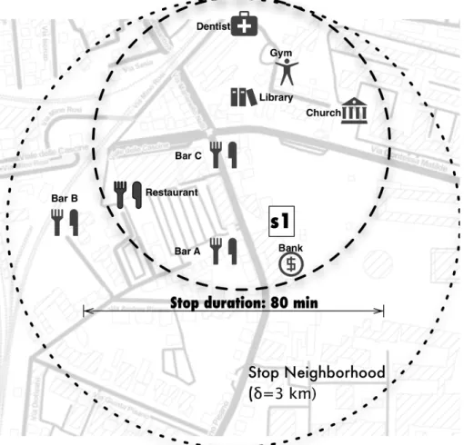
• Semantic Enrichment of GPS Track [24],[16]: spatio-temporal datasets proved to be very useful to analyze and understand mobility behaviors of cit-izens but, at the same time, poor in terms of semantics: we can infer where and when people move, but not the purposes of their movements. This work is a step in the direction of semantic enrichment of mobility data. We de-fine a method, called ACTIVE, to associate the trajectories stops to the most probable activity performed, analyze the Points of Interests in the stop neigh-borhood, and exploit the gravity model. Experiments done show the good accuracy of the algorithm when compared to a ground truth.

(16)

• Route Planning exploiting Wisdom of the Crowd [31]: the data in-tegration process could also be viewed as a cycle. The information gain of the first loop (e.g. map matched GPS data) becomes a data source itself, to be combined with further mobility data. Map matched trajectories repre-sent the most precise proxy of road network usage, providing the possibility to learn how drivers route across the network to reach a destination. Mod-ern route planners – such as personal navigation assistants – generally return routes that minimize either the distance covered or the time traveled. How-ever, these routes are rarely considered by people who move in a certain area systematically. Indeed, due to their expertise, they very often prefer different solutions. In this paper we provide an analytic model to study the deviations of the systematic movements from the paths proposed by a route planner. We extract the systematic movements from a set of drivers and translate them into sequences of road segments, in order to compare such sequences with the shortest/fastest path relative to the respective systematic movement. Our re-sults show that about 30-35% of the systematic movements follow the shortest paths, while the others follow routes which are on average 7 km longer. Fig. 1 shows a general schema describing the contributions provided by this thesis and the relations among them. As depicted, the point-to-segment matching method and travel time estimation algorithm is the starting point for all the subsequent con-tributions. In fact, a point-matching task is involved in all the subsequent works. Furthermore, results from the application of Time-Aware map matching algorithm are also part of the input of data for the analysis of users’ route planning policies.

This thesis is organized as follows: in Part I there is a review of state-of-the-art works regarding the challenges faced. Pstate-of-the-art II describes and explains the main contributions of this thesis. Part. III summarizes some preliminary results obtained on new challenging analytical problems that, in part, follow the above mentioned achievements up, and in part explore different directions in the domain of Mobility Data analysis .

(17)

Introduction 15

Mobility Big Data

Road Network Travel Times Estimation Time Aware Map Matching Route Planning exploiting Wisdom of the Crowd Semantic Enrichment of GPS Track

Figure 1: Workflow of the thesis. The first result has been the base to explore Mobility Data Integration research field, thus starting an integration process where the result of a first step is itself a further data source.

(18)

(19)

Part I

(20)

(21)

1 Related Works

In this era of Big Data a huge amount of information are available from every single citizen of our strong connected world. A simple smartphone can collect data enclos-ing different kinds of informations: a big part of these are related to mobility. A smartphone is connected to networks, such as GSM, GPS, Internet (and then social networks): each of them can give us information about where, what and why the user is moving across space and time. Understanding human mobility is an important challenge, and the comprehension of such phenomenae have conquered the attention of many scientific communities: physicists, sociologists, are working together with computer scientists to take advantange of the chance given by the increasing amount of easy-collected Mobility Data. The knowledge on human mobility - fundamental for application such as urban planning,traffic forecasting or spread of biological and mobile viruses - is getting bigger, helping decision makers on their job. To give a quick overview, in a recent and popular study regarding the diffusion of Ebola virus ([29]), authors developed a statistical model by integrating daily airline passenger traffic worldwide and the disease model obtained combining the community, hospi-tal, and burial transmission dynamics. Mobility data analysis have been involved in the understanding of a case that gained the attention of all the main institutions all over the world, and the solution proposed has been built through the aggregation of multiple types of data.

Data integration has a key role indeed. The combination of different data sources increases the value of the extracted knowledge, even though the integration process is often not trivial. In the following sections there is a review of state-of-the-art methods regarding the Data Integration challenges faced in this thesis.

First contributions in the field of Mobility Data Analysis regarded the process of Trajectory Mining. When the possibility to analyze huge dataset of spatio-temporal data arose, many researchers started to develop methods and algorithms to find

(22)

pat-tern and common behaviors among those datasets. A spatio-temporal trajectory can be represented as a sequence of points (x1, y1, t1),(x2, y2, t2) ... (xn, yn, tn), where

(xi, yi) is the spatial location, consisting in longitude and latitude, and ti

repre-sents the timestamp, i.e. the time when the location (xi, yi) is recorded. Trajectory

mining have been defined by extending traditional Data Mining techniques to such spatio-temporal data: clustering, join, classification, are now operation available also over trajectory data. One of the first paper in this field is [27], where Trajectory Pattern Mining has been proposed as a model able to provide a concise description of frequent behaviors in term of both space and time. Pattern discovery among trajectories was also the topic of [30], where authors addressed the problem of mod-eling subgroups of trajectories that exhibit similar movement and proximity for a certain amount of time. Once introduced the concept of spatio-temporal pattern, the next challenge has been to go up through the possible semantic layers of Mobility Data. This has lead to the ipothesis of a framework able to extend the concept of mobility pattern: mobility data sources are nowadays manifold, describing different meanings of human mobility: it is not only where and when we go, but also why

we go, and what we are going to do. The wide field of Trajectory Data Mining can benefit from the evolution of Data Integration processes. In [50] authors propose a method to estimate traffic conditions based on GPS trajectories, historical data, and contextual informations such as the Point of Interests associated to each road segment. The complex task of Trajectory Classification (see [52], [36]), that is the process of recognize and asses the characteristics of a trajectory (e.g. still/moving, transportation modes, activities performed) is already taking advantage of POIs to train the machine learning models –i.e. Conditional Random Fields, Hidden Markov Model- involved in the classification process.

The work done in this thesis aim to face the challenge of enriching the semantic informations extracted from mobility data through the integration of multiple data sources. The focus has been posed on some particular open problems, which are defined in the following subsections.

1.1 The Map Matching Problem

Map matching is the process of associating a sequence of spatio-temporal points to a connected sequence of road segments, thus enriching raw data with the semantic layer provided by the roadmap and all the contextual information associated to it. Although it is a classical and well known task in GIS literature, the map matching problem still represents an important and a valuable challenge. The map matching

(23)

1.1. THE MAP MATCHING PROBLEM 21

problem can be treated at two different scales, depending on the characteristics of input data, which can be made of either high-frequency or low-frequency samples of the real position of the recording device. The former is mainly treated in the field of Personal Navigation Assistants, where the device is able to identify in real time the road where the user is traveling. The latter is common for applications dealing with smartphones or GPS-equipped black boxes installed vehicles for security or insurance purposes. This kind of devices sample and store their location at a lower frequency to limit the battery consumption or to reduce data exchanging between the device and the server that stores the information. The result is a coarse-grained GPS data, harder to deal with but still with high value: this data represents the most reliable proxy for road network mobility. One important issue introduced with low-frequency samples is path reconstruction. After mapping single points to the road network, between two consecutive locations there might be a significant gap, therefore requiring strategies to reconstruct the path traversed by the vehicle or the individual.

Map matching algorithms are classified according to three categories: global, incremental and probabilistic algorithms. The focus of this review is on global and incremental algorithms, since the probabilistic approach (e.g. Kalman Filters) is used to tackle the high-sampling rate map matching problem.

Global algorithms solve the problem by considering the entire trajectory, the solu-tion is obtained by searching the closest path in the map w.r.t. the input trajectory. In [4] there is a first example of global matching algorithm: map-matching is the result of a spatial query, the resulting road network path has the minimum Fr´echet distance w.r.t to the input trajectory. Fr´echet distance is a mathematical model used to compare two curves: in its more common and easier illustration, it is viewed as the minimal length of a leash between a dog and his owner, whom are walking on different curves. The complexity of this approach is quite high: O(nmlog2nm), withn as the number of trajectory points andmthe number of road network edges. In [12] a more efficient version of Frchet distance computing algorithm has been provided.

The main issue for global algorithms is the purely geometric approach. All the characteristics of the road network are ignored, the matching is only based on the research of a similar curve. It is obvious to notice that there will never be a low-sampled trajectory completely equal to a path in the network: this means that there is not a precise definition of the optimum to reach. In [10] Frchet distance is even used for a quality evaluation of the results obtained. The incremental approach for low-sampling map matching is based on joining optimal local searches. The local optimum is represented by the most probable path between two consecutive matched GPS points. IVMM algorithm ([63]) is one of the state-of-the-art incremental map

(24)

matching algorithm we used to compare the results of our work. The matching process is done through consecutive steps; first of all, a preliminary refinement is done by dropping vertex according to a spatial range query. Then, the matching probability is computed assuming the GPS error with a normal distribution; this position probability is combined with a transition probability, that is the ratio be-tween the euclidean distance of two candidates and their shortest path distance on the road network. Furthermore, a temporal analysis is also considered: the cosine similarity between the travel-time (according to road speed limits) of the shortest path analyzed and the real time difference between the two GPS points. The last step of IVMM is a mutual influence modeling, used to decide the path between each consecutive points by considering also at the global trajectory. In this approach, there are several not verified assumptions: first of all a driver should always follow the shortest path. Moreover,the radius of the range query is arbitrary and the GPS error is assumed as Gaussian, with fixed parameters. Furthermore, the travel-time of road edges is obtained according to road speed constraints. These constraints, es-pecially on a city road network, could be considered as arbitrary. In [18] a method to get rid of this assumption has been proposed: a gravity model is used to associate a GPS point, with his speed, to a road segment, choosing between the k-nearest neighbor.

A particular case of probabilistic approach used to deal with low-sampling rate data is [40], where authors developed a map matching algorithm based on the well known Hidden Markov Model. This algorithm has a weak point on its highly dependance on two parameters, both of them obtained from the ground truth, i.e. from the road segments actually traversed from the vehicle; this kind of data are not available in a real application scenario of a map matching algorithm. Another factor of weakness is its complexity: for each trajectory, Viterbi algorithm takes O(|C| ∗ |S|2_{) to find a} solution, whereC is the set of transitions between segments and S the set of all the segments candidates to be matched with a point of the input trajectory. It is worth to point out that for all the transitions in C the shortest path is computed, thus adding the complexity of this computation, that is P

p∈P

|Cp|2∗(|E|+|V|log|V|). Here

Cp is the subset of candidates segments associable to the single GPS point p. In

the next part of this thesis there is a comparison between a new approach for solv-ing the map-matchsolv-ing problem, namely ”Time-Aware map matchsolv-ing algorithm”, and the state-of-the-art methods reviewed above. The comparison has been made on three different datasets, either with a ground truth (ACM sigspatial cup 2012 []) and gathered from on board GPS devices. The validation of a map-matching algorithm designed to process a real GPS dataset is not trivial indeed. Datasets ac-tually available (either public or not) are usually stored without the roads traversed

(25)

1.2. HUMAN ACTIVITIES RECOGNITION 23

by vehicles that have generated the GPS tracks; in this scenario, checking whether a map-matching is correct or not is not possible. Hence, every method based on a machine learning approach can not be exploited on such GPS datasets, where a ground truth is not provided. However, the validation of Time-Aware algorithm consider both -ground truth available/not available cases - in order to provide a detailed overview of the goodness of its approach.

1.2 Human Activities Recognition

The importance of Mobility Big Data is represented by the information they en-capsulate: the traces of people’s activities. All of our movements are done with a specific purpose. The understanding of why a person moves is the last frontier in the semantic enrichment of Mobility Data. In other words, inferring the activity carried out by a moving individual from the raw mobility data, in absence of any metadata about the intention of user, is a challenging task that can bring highly innovative contribution to the study of human mobility behavior. Nowadays, several applica-tion areas would benefit from an extensive study on people’s activities such as traffic management, public transportation, commercials and advertising, security and po-lice, hazard evacuation management, location based services and so on. Despite the fact that data collected from mobile devices is increasing its location accuracy, it is not improving in the same way their quality in terms of semantic richness. This means that there is a semantic gap between raw data collected from mobile devices and the personal activity that generated the traces. As a consequence, techniques to semantically enrich the collected data are necessary to (semi-) automatically infer the person’s activity given her/his location traces.

Inside this scenario, it is possible to address two different research trends: (1) the detection of stops in trajectory data and the relative association of a place and (2) the inference of the activity performed during the stops.

Regarding the first trend, it is worth to recall the pioneering work of [53] where authors propose a conceptual model for semantic trajectories. While trajectories are defined as a time-space function that records the changing of the positions of an ob-ject moving in space during a given time interval, semantic traob-jectories are defined as sequences of stops (where the moving object stays still during a time interval) and moves (the part of a trajectory where the position of the object changes). The basic assumption behind the notion of stop is: the place where a person stops is of some interest for her/him. Therefore, each stop is associated to an activity. The inference of the kind of activity performed requires the definition of a relation between Mo-bility Data and domain knowledge base. Such informations have two main sources:

(26)

(i)user direct annotation and (ii) Point-Of-Interests (POI) dataset. Many reserches are based on volunteer’s tracked data, where users provide a complete survey of the activities associated to tracking data, while a completely different approaches relies on the identification of the POIs visited by the user during each stop.

The association between a POI and a trajectory stop is the objective of several approaches, ranging from the simplest (associating the closest like in [43]) to more sophisticated proposals, reported in [46]. However, most of the approaches do not explicitly consider the temporal validity of the association (i.e. if the POI exists or it is accessible during the actual stop), neither the probability value associated to each stop-POI pair, nor the concept of activity.

The identification of mobile activities from trajectories of people is not new in the literature ([64]). A trend of research is devoted to the identification of trans-portation means like the work [65]. Using speed, acceleration and speed change rate, authors first detect the positions where the movement switches between walking and non-walking. In a second step, they refine the non-walking segments into segments characterized by the other transportation modes: bicycle, bus, and driving. They use a combination of techniques, from supervised learning to decision tree inference, and add a post-processing step to improve the accuracy of the segmentation. The post-processing step relies on a graph that contains commonsense constraints about the real world and typical human behaviors.

Another trend is concentrating on the identification of the activity during a stop. In [59] authors present a method to automatically extract sequences of activities from large set of trajectory data. The assumption is that activities may be carried out at a POI during a stop in the user trajectory. The association between a stop and a POI - as in our case - is crucial and may depend on several factors. One is the distance between the POI and the trajectory and the other is the duration of the event. They base their approach on the concept of influence distance for associations among trajectories, POIs, and activities. Influence is a distance based measure, such that a trajectoryT can only be associated with a POI if there exists at least one point onT that isinfluencedby the POI. They use the Voronoi diagram as a division of the area where each cell represents the influence area of the POI. They test their algorithms using synthetically generated trajectories dataset with the POIs collected in a specific area in California. Naturally, the drawback of this testing is that there is no real validation of the method since there is no proof of the correctness of the inferred POIs.

The work of [33] is again in the direction of inferring activities from users trajecto-ries. This paper presents an approach using spatial temporal attractiveness of POIs to identify activity-locations and durations from raw GPS trajectory. The algorithm they propose finds the intersections of trajectories and spatial-temporal

(27)

attractive-1.3. MOBILE PHONE DATA KNOWLEDGE EXTRACTION 25

ness prisms to indicate the potential possibilities for activities. The experiments use one months GPS trajectories from 10 volunteers where they show an high accuracy of the method.

[35] propose a method for user intention recognition in the mobile case. They pro-pose a framework where movement information through GPS data in used by a system of production rules and classification techniques for the intention recogni-tion process. This approach mainly focuses on movement features such as speed, angles etc. to segment a trajectory, whereas approach we present in Chapter 4 relies on the identification of a stop where no GPS signal have been detected, then it infers the visited POI and consequently derives the user activity.

A different approach is [61]. Here the focus is not on the analysis of the single user but an aggregate vision of regions. Trajectories, POIs and road networks are combined to definefunctional regions. The result is a set of regions represented by a distribution oftopics(or functions), where a topic is a POI category. With this work authors aim to help people to easily understand the complexity of a metropolitan area. The results are applied to different fields, such as urban planning, location choosing for business, advertisement casting and social recommendations.

In the same direction there is the work of [60], where authors propose an activity discovery method for moving objects based on collaborative filtering. After having generated the objects activity sequence and abstract the corresponding features, they build a three dimensional matrix (object identification, hot region, and se-quence). On the basis of this matrix they compute objects interest degree to each hot region and generate an object-region interest degree matrix. Combined with collaborative filtering, similar objects can be queried and their common interest-ing activities can be found. Furthermore, they propose a recommendation system based on the K-nearest neighbor algorithm by which a series of potential interesting activities can be recommended to the moving objects.

1.3 Mobile Phone Data Knowledge Extraction

Mobile phone is the main character of this Big Data era. The penetration of such device have continously increased during the past decade, delineating a trend that is still running: by 2020, 90 percent of the world’s population over 6 years old will have a mobile phone. During every moment of people’s life, a mobile phone is present. Mobility is not the only feature of human behavior that can be derived from mobile phone data, even though is the most fascinating one.

(28)

Figure 1.1: Comparison between an user actual trajectory (dashed line) and CDR generated by his/her calling activity. It is only possible to derive the presence of the user over the spatial region A,B,C, i.e. the area covered by the tower the phone was connected to during the call and SMS he/her performed. Sometimes also a LAC Update is available: it represents a Location Area Change, i.e. phone is connected to a tower that is in a different area w.r.t. the previous tower it was connected to.

be collected in two modalities: on Network-side modality the provider records such data for specific billing purposes; in the Handset- side modality the data are collected by phone sensors (GPS,Wifi,Bluetooth,...). So far, research works in this field use to identify Mobile Phone Data as the Network-side Data. The main element of this data type is the Call Detail Record (CDR): it represents an user event that must be billed, i.e. voice calls, SMS, MMS and so on. Mobility knowledge contained in CDR Data has some particular weaknesses to deal with: the completeness in terms of space and time is not guaranteed. While GPS data can be properly resumed by means of trajectories, this is not possible with CDR Data. The position of an user over space and time is known only when he/her is calling or sending SMS. This lead to a coarse mobility data, not representable in terms of user trajectories. Moreover, the spatial granularity is defined at a GSM-tower level: for each event, a CDR contains the GSM tower where the phone was connected to. Since the coverage of a tower is in the order of square kilometers, even the concept of georeferenced point related to a billing event is not proper. Even though these lacks of quality (see Fig. 1.1), by means of Call Detail Records (CDR) Mobile operators are collecting the most precious source of mobility data, since it is covering the globality of world’s population.

Altough the different spatio-temporal quality of CDR, there are plenty of works about mobility based on Mobile Phone Data. In [34], CDR regarding an one year long (October 2008-September 2009) user activities have been used to observe traf-fic pattern on the road connecting the two main city of Estonia. In this context,

(29)

1.3. MOBILE PHONE DATA KNOWLEDGE EXTRACTION 27

authors built a traffic monitor based on mobile phone activities from half a billion clients: the potential of this research field relies exactly on tha high number of users involved. Furthermore, the availability of data from a wide time range lead to a pre-cise users profilation. This improve the quality of traffic monitoring by highlighting, for instance, the composition of traffic in terms of users type: residents,commuters or visitors. Another approach in this direction is the one from [11]; here, authors pro-vide techniques to extract mobility patterns from mobile phone traces. Moreover, a valuable comparison between mobile-phone-based and odometer-based mobility measures has been performed, in order to validate and analyze the quality of the results obtained. Both of the works introduced rely on users profiling, that is a task useful to classify users according to their visited location. The purpose of such pro-cess is to further enrich the mobility analyses by extending the semantic of detected patterns, i.e. to distinct between patterns of residents and commuters w.r.t. to a selected geographical area. Users profiling is one of the task accomplished in [39]: CDR are used to compute the two most visited location for each user, inferring those locations as Home and Work. This result is further extendend and refined in [25], where a framework to detect residents,commuters and visitors is provided.

(30)

(31)

Part II

Data integration: boosting the

power of data

(32)

(33)

31

Every kind of mobility data has its type and its meaning in terms of knowl-edge. Each one of them express a different dimension, enclosing a particular char-acteristic of every-day life activity; the idea leading this thesis is to exploit this multi-dimensionality to better understand the big picture of human mobility. The combination of such dimensions is still a demanding challenge, either for method-ological and structural reason. The importance of such challenge is clear if we consider how many kinds of Mobility Data we produce with our most used device; in fact, a simple smartphone has lot of sensors: GPS, accelerometer, Wifi, and, of course, GSM antenna. All of them are proxies for a specific type of mobility data.

When a GPS device records a point (this process is called fix), it is able to get data with features such as (latitude,longitude, heading,timestamp,instant speed ). When a call starts from a phone, the event is recorded by the GSM tower the phone was connected to, thus identifying a wide area the user visited at a certain timestamp. While GPS points are the most precise representation of a movement across space and time, GSM data have a higher pervasiveness but a rougher space precision. However, all of these data types do not provide any other semantic layer. A geotagged tweet, conversely, contain a text associated to the place the user was while writing. On Fourquare, users check in and specify the place they are both in terms of spatial reference and Place of Interest visited, and so on. Manifold are the example of semantic associated to spatio-temporal data; the data revolution happening nowadays is owing to spatio-temporal data the possibility to localize in space and time many events that represent different aspects of our lives.

Following, contributions to the data integration challenge - developed during the course of this Ph.D. - are described.

(34)

(35)

2 Exploiting GPS Data to assess

Road Network Travel times

The assessment and consideration of traffic conditions are the keys for develop-ing intelligent transportation services, such as, route planndevelop-ing, traffic flow analysis, route path discovery, to name a few. In this context, the time taken by a vehicle to traverse a road segment can vary depending on the time of the day and, more critically, road segments can even be unavailable during certain time intervals. For example, to compute the fastest route between two points within a time-dependent network, we take into account the departure time, since road traversal time may vary along time. Thus, key methods for intelligent transportation service, such as routing, shortest path,KNN, should be revisited and adapted according to this new constraint. The proliferation of GPS-enabled devices is allowing the production of a huge amount of location trajectory data. However, trajectory data collected from GPS devices suffers from two problems: (i) low sampling rate data (due to aggre-gations executed by the device to save communications with the base station), and (ii) error in GPS observations, which imply that most detailed information about the exact movement of the object is lost and great uncertainty arises in their routes. Clearly, this kind of uncertainty severely affects the effectiveness and efficiency of underlying methods such as, indexing, querying and mining. The proposed method allows to compute average speed for each segment of the road network in distinct time periods, providing a comprehensive view of the traffic conditions.

(36)

2.1 Problem definition

The aim of this work is to find a methodology to compute the real speed of each segment in a given road network, using the observation (i.e. points) coming from GPS devices. By definition,such observations are affected by errors. Then, from the speed computed, generate travel-time functions to compose a time-dependent network. Several methods in literature consider a Gaussian distribution of the GPS error; this assumption could be not true and therefore an innovative way to consider the problem is needed.

Below we provide a formal description regarding the speed estimation for a road segment.

Definition 1. Given a set of observations O={o1. . . om}where oi = (pi, di, si)has

its spatial position pi, its direction di and its speed si, a set of road segments R =

{r1. . . rn} and having an function σ(oi, R) = (w(oi,rj), rj) assigning the observation oi to the segment rj ∈ R with a confidence value w(oi,rj), it is possible to estimate

the speed over the segment as:

Speed(O, R, rj) = P oi∈Oj w(oi,rj)·oi.s P oi∈Oj w(oi,rj) Where Oj ={oi|σ(oi, R) = (w(oi,rj), rj)}.

Following, we define a method to estimateσ(oi, R) function without any

assump-tion on error distribuassump-tion.

2.1.1 The gravity model

Having the set of observationsO and the set of segmentsR we define theattraction

of a segmentj for a point i as: w(oi,rj)=w

d (oi,rj)·w θ (oi,rj) where • w₍d_o i,rj) = 1− dist(oi,rj) P rk∈R dist(oi,rk); • w₍θ_o i,rj) = 1− ang(oi,rj) P rk∈R ang(oi,rk);

Furthermore,distis the Euclidean distance between a point and a segment andang is the absolute difference between the direction of the point and the direction of the segment. The direction is measured in degrees, where 0 degrees indicates north direction and 180 degrees is south directions. For the every observation, this value comes directly from GPS device. Therefore the force of attraction of a segment over a point is defined by the combination of these two dimensions as:

(37)

2.1. PROBLEM DEFINITION 35

Definition 2. Having an observation oi ∈ O and a segments rj ∈ R the gravity

force functionGF(oi, rj) =wd₍_o_i_,r_j₎×wθ₍_o_i_,r_j₎. Finally the point is assigned to segment

with the most powerful force: σ(oi, R) = argmaxrj∈R(GF(oi, rj)).

This methodology will be referred as Gravity Model and we consider to have a functionGM assignO,R(oi) = hoi, σ(oi, R), w(oi,σ(oi,R))iwhich returns, in other words, the triple t∈assignments where t.o=oi.

To better understand the idea under the definitions, we present a complete ex-ample (Figure 2.1) of how the forces are computed and how the points are attached to segments. In Figure 2.1 a sample of points and segments is shown, the points are

Figure 2.1: An example of observations and segments used to explain the gravity model (Top) and the two distances: Euclidean distance (right) and Angular (left) between each point-segment pair.

attracted by all the segments with different forces and suddenly they fall over one of them. For example the point P1 undergoes the following forces:

GF₍d_o 1,rab) = (1−10/100)(1−39/200) = 0.9∗0.305 = 0.2745 GF₍d_o₁_,r bc)= (1−10/100)(1−4/200) = 0.9∗0.98 = 0.882 GF₍d_o₁_,r cd) = (1−28/100)(1−66/200) = 0.62∗0.67 = 0.4154 GF₍d_o 1,rce) = (1−28/100)(1−2/200) = 0.62∗0.99 = 0.6138 GF₍d_o₁_,r hc)= (1−8/100)(1−46/200) = 0.92∗0.77 = 0.7084 GF₍d_o₁_,r_hf₎= (1−9/100)(1−2/200) = 0.92∗0.99 = 0.9108 GF₍d_o₁_,r gh) = (1−9/100)(1−41/200) = 0.99∗0.795 = 0.78705

Therefore the point is attracted mostly by the segmenthf or more formallyσ(oi, R) =

(38)

2.1.2 Candidate selection

The Gravity Model is applicable over the whole road network, but in real applications the set of segments to be considered is too large. For this reason we present two different methods to select the set of candidate segments. The first one, already used in previous works in literature, uses a buffer around the points selecting only the segments with a distance which is lower than a certain threshold. Instead, the second method uses the concept of nearest neighbor, taking only the first k segments near the point.

2.1.3 Buffer method

All the most used approaches for the assignment of a segment to a GPS fix are depending from a search buffer: the segment, or the candidates, are initially chosen from all the segments contained in a circumference of radius . This parameter is very application dependent and usually can not be derived from the real observa-tions, because the ground truth is not available, and affect greatly the result of the point-segment process. Moreover using a buffer the error distribution is assumed to be normal which, as already said, is a strong assumption. For example the presence of buildings affects the precision of the GPS and therefore all the observation can be affected to a bias. In Figure 2.2 (on the left) two examples of road network is shown, here the buffer method selects a number of candidates which can greatly vary in different context (e.g. urban or sub-urban areas).

Figure 2.2: Two examples of road network and the candidate selection using the two different method: a buffer of 30m (left) and the 3 nearest neighbors (left).

Another effect of this method for the candidate selection is the fact that some points which has no segments inside the buffer are discarded, this leads to a reduction of the set of observation used.

(39)

2.2. FROM SPEED ESTIMATION TO TRAVEL TIME 37

2.1.4 K-Neighbor method

Instead of considering a fixed buffer with the limitation described before, we defined an innovative way to select the candidates choosing the k nearest neighbors of a point. Here the only parameter needed iskand we will show in the validation section how this affect the results increasing the accuracy compared to the classical buffer method. In Figure 2.2 it is possible to see another advantage of this method: in factkis the exact number of segments considered for every point-segment matching leading to a controlled complexity in time and space of the algorithm.

2.2 From speed estimation to travel time

The structure of a dependent network can be modeled by a TDG (a time-dependent graph) where the vertices represent the network junctions, starting and ending points of a road segment (e.g. a street or an avenue) and the edges connect vertices (depending on the application, additional points can represent a change in curvature or in maximum speed of a segment). The cost (time) to traverse an edge is a function of the departure time. A TDG G = (V, E, C) is a graph where: (i) V = {v1, . . . vn} is a set of vertices; (ii) E = {(vi, vj) | vi, vj ∈ V, i 6= j} is a set of

edges; (iii) C = {c(vi,vj)(·) | (vi, vj) ∈ E}, where c(vi,vj) : [0, T] → R

+ _{is a function} which attributes a positive weight for (vi, vj) depending on a time instantt∈[0, T]

and whereT is a domain-dependent time length. In other words, a TDG represents a road network with the traffic information about it including as the weight of the edges. In many cases the traffic information is not directly available or not really reliable, but the structure of the road network and a trajectory dataset are available. In following, we show how the speed estimation, using the gravitational model, gives us the support to build the functions in the set C of a TDG from the available trajectory points. More specifically, we describe how to convert the average speed of a segment of sequence of time intervals, in a travel-time function that is piece-wise linear. We choose piece-wise linear functions because it is easy to check if these functions attend the FIFO property. We call this algorithm GenerateTravelTime: given a road segment and a timestamp, it returns the travel time of the segment, calculated using the average speed of that segment at that time. Furthermore, if we use the average travel-time for each time partition, we create a piecewise constant travel-time function, that means the function does not attend the FIFO property in all decreasing pieces. Figure 2.3 (left) shows a function obtained by two steps: the first (left) approximating the various pieces and the second (right) which ”smooths” the function using a linear interpolation for the middle points. Having the function for each edge, methods as [42] are able to find the best routes considering the

(40)

dynamic travel time. We call a time-dependent network a road network which has a time-dependent function as the weight of its segments, instead of a constant value. To exemplify the fastest path problem in a TDG, consider that someone wants to

Figure 2.3: On the left, an example of a function build in the first step with the travel-time averages. On the right, a result of the transformation applied in the second step.

go froma todat 16h. The best choice in this case, i.e. the path that has the lowest cost, is< a, b, c, d >. Travel froma tob takes 15 minutes, to go frombtocat 16h15 takes 15 minutes and to go from c to d at 16h30 takes 20 minutes, then the path < a, b, c, d > takes 50 minutes. Consider now a departure time ts = 10h, a path

< a, b, c, d > takes 70 minutes and a path < a, c, d > takes 45 minutes. Thus, the fastest path at 10h is < a, b, c, d >, but at 16h the best choice is to follow the path < a, c, d >.

Figure 2.4: The result of the speed estimation for a the same portion of the road network at different time of the day: 4am, 6am, 10am and 1pm. The light green represents high speed and the red represents a low speed.

2.3 Validation

In this section we will validate and evaluate the proposed Gravity Model with the two candidate selection methods in order to study how the accuracy changes. As

(41)

2.4. PERFORMANCES STUDY 39

already said the ground truth is not available in real data, for this reason we created a synthetic dataset using an up-to-date simulator and perturbing the resulting dataset. In this way for each simulated observation we have the real segment which generated it. In the following we first describe the way we produced the data and then a complete study of the methods results will be presented.

2.3.1 Generation of synthetic observations dataset

In order to validate our method we generated a synthetic dataset of observations. We used theSUMO simulator [8] for generating a synthetic dataset of trajectories. We used, as input, the road network of Pisa and surrounding area extracted from

Open Street Map. In order to replicate the same condition we have in the real dataset (as we show in Section2.5), we have used a set of parameters extracted from previous studies published on the same dataset [26] such as the sampling rate between 30 and 90 seconds. We generated the observations of 2000 vehicles moving on the network for a day obtaining 314785 points perfectly positioned on the road network. To simulate the error of the GPS devices, we added some noise at each observation: (i) the spatial component of the observation is moved by a random value considering a normal error distribution with a variance of 45 meters; (ii) the orientation is changed by a random value considering a normal error distribution with a variance of 90 degree. It is important to notice that these values are extracted by an empirical study over the real dataset which does not contains any information about that, therefore heuristics were applied in order to estimate these errors. Moreover, even if our methodology does not need to consider a normal distribution of the error, we decided to apply it to the synthetic data because we do not have information about buildings or other conditions interfering with the GPS signal.

2.4 Performances study

The simulated observations allow us to validate our methodology knowing for each point the segment which generated it. We used two measures in order to evaluate the methodology: precision and accuracy:

precisionO,R =

|{oi|GM assignO,R(oi) =Belong(oi)}|

|O|

whereBelong is the real information coming from the simulated data. error rateO,R(rj) =

Speed(O, R, rj)

(42)

whereSpeed(O, R, rj) is estimated using the speed function obtained from the

Gen-erateTravelTime algorithm and RealSpeed(rj) is the speed used in the simulation

for the segment rj.

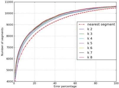
Analyzing how the precision varies using different parameters for the two candi-date selection methods, we obtained the results shown in the following table:

Table 2.1: Precision comparison

Range buffer precision Nearest k precision

10mt 15.2% k 1 69.0% 20mt 29.7% k 2 75.6% 30mt 42.4% k 3 77.5% 40mt 72.0% k 4 78.6% 50mt 74.8% k 5 79.1% 60mt 75.2% k 6 79.3% 70mt 75.9% k 7 79.4% 80mt 76.0% k 8 79.4%

Table 2.2: Comparison between precision obtained with range-buffer search and Nearest k search.

As expected the buffer method converge to a good result approaching the vari-ance used in the simulation (45mt) but this put in evidence the fact that without a good estimation of the possible error it is difficult to obtain such results, and as described before this information is usually neither reliable or unverifiable. On the other hand theKNN method got better result since the beginning due the fact that it is more adaptive to different context, here the method obtains a precision which converges rapidly to a value of 79.4% highlighting the fact that it adapts better to every context in the road network. Even though this is not the most important result to us, it is a value useful for a comparison with other work in this field; the online algorithms like [40] have a really high precision (over 90%) when used with sampling rate 1 Hz and the measurement error is low, but with low sampling data the precision decrease significantly: with our same values of sampling and error vari-ance, the precision of the algorithm mentioned is around 50%.Moreover selecting a value of k we select exactly that number of candidates without losing the control of the performances as it happens using the buffer method. We can see in Figure 2.5 the cumulative distribution of the KNN method error percentage, varying the pa-rameter k. This plot shows how 77% (8500) of the segments has an error in the speed estimation under 20%. As we saw in the precision comparison (2.2), the error rate

(43)

2.5. REAL CASE STUDY 41

Figure 2.5: Performance of Gmatch for different value of k

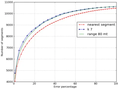
converge giving strenght to the approach. Another interesting aspect is that the error is usually on the low speed roads, therefore the average speed estimation error in absolute terms is 6.1km/h, and considering the average speed of all the network segments of 58.32 km/h, it is only a an average error of 10.4%: this is the main result of our work, since our goal is to estimate the speed of each road segment. Comparing the error rate of the buffer method using 80mt and the KNN method with k=7 we can see in Figure 2.6 that the results obtained are better also in the evaluation of the speed.

Therefore we can conclude that the Gravity Model not only is better using the KNN candidates selection but it is very simple to use overcoming the problem of knowing or estimating the error variance of the application scenario.

2.5 Real case study

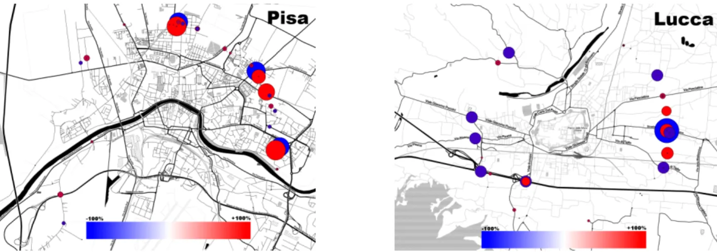
In this section we present the results of our method applied to a real dataset of GPS observations of 30000 real car users in Tuscany in a time period of 5 weeks covering different kind of territories such as urban and suburban areas. This is a sample of data obtained by a private company employed specifically as a service for insurance companies and other clients called Octo Telematics. We processed this dataset of observations (Fig.2.8(left)) using the presented algorithms and in the following we will show the results obtained. As described above the GMatch is applied using the

(44)

Figure 2.6: Comparison between precisions obtained by using the KNN method with k=7 and the buffer method using a threshold of 80mt.

KNN candidate selections setting k=7 and dividing the dataset into sub-datasets considered one hour time intervals. Then, applying the GenerateTravelTime, we build a function for each segment extrapolating the speed discovered in each interval. The result for each road is shown in Figure 2.7 where the travel time changes in time, in this case looking to a specif roadStrada del Monte Serra the time needed to traverse it is lower in the morning and higher in evening, especially if the departure time is around 8:00pm.

In Figure 2.4 we show another real example of how the speed change in time on a set of road segments in order to show how the right assignment lead to a consistent situation: here during the early morning at 4:00am the speeds are higher (light green) especially on the highway located at the bottom of each figure, than going on with the time, the speed over the segments becomes slower and slower (from green to red) reaching the 1:00pm where the traffic decrease the speed greatly on the main roads: the highway and the roads directly connected with its entrance/exit. This represent our best result in fact it can be done thanks to the functions computed over the real observation which are attached to the right segments as shown in the validation section.

Moreover in Figure 2.8(right), in order to assure the correctness of the result, we compared the distribution in time of the number of cars with the average speed on the network. It is important to see how the average speed increase when the number

(45)

2.6. SUMMARY 43

Figure 2.7: An example of real travel-time functions. On the left, travel time gen-erated using speed estimation from Strada del Monte Serra, Pisa, in the morning. On the right, travel time from speed estimation from the same road at night.

of cars decrease and vice-versa.

Figure 2.8: The dataset used (left) and the average speed of the network compared to the number of active cars during the day (right).

2.6 Summary

In this chapter we proposed a gravity model method for computing road segment average speed from trajectory data. In sequel, we show how to generate travel-time functions from the computed average speeds. Our approach allows extracting a set of speed functions, which can represent precisely the traffic conditions in time and space, without considering strict assumptions on error distribution. The proposed method accuracy is validated using a synthetic and a real dataset showing that it leads to a more realistic results. We shown also how the results obtained give the possibility to improve existing methods for routing, KNN, and shortest-path algorithms which take advantage of the time-dependent network.

(46)

(47)

3 A Time Aware Map Matching

Method to enrich Raw

Spatio-Temporal Trajectories

The widespread diffusion of location devices for personal usage, from GPS navigators to location-based services on smartphones, are making this decade the era of Geo-Spatial Data. Coupled with the novel technologies for storing and processing large streams of data, this phenomenon is leading to the collection of massive datasets of GPS (or GPS-like) traces describing the movement of people and vehicles, as well as to the development of analysis methods and applications that use such information to extract useful knowledge. Some examples are provided by the current studies on knowledge discovery from spatio-temporal data, based on methods like trajectory pattern mining [27] or flock mining [41]. These approaches rely only on spatio-temporal features of raw data without considering any geographical characteristic, such as the features of road network.

In this context, map matching, i.e. the process of associating a sequence of GPS points to a connected sequence of road segments, gives us the chance to enrich raw data with the semantic layer provided by the road map and all contextual information associated to it, e.g. the presence of speed limits, attraction points, changes in elevation, etc.

Although it is a classical and well known task in GIS literature, the map matching problem still represents an important and a valuable challenge. The map matching problem can be treated at two different scales, depending on the characteristics of input data, which can be made of either high-frequency or low-frequency samples of the real position and movement of the device. The former is mainly treated in the field of Personal Navigation Assistants, where the device is able to identify in real time the road where the user is traveling. The latter is common for applications

(48)

dealing with smartphones or GPS-equipped black boxes installed vehicles for security or insurance purposes. This kind of devices sample and store their location at a lower frequency to limit the battery consumption (e.g., with smartphones) or to reduce the traffic of data between the device and the server that stores the information. The result is a coarse-grained GPS data, harder to deal with but still with high value: this data represents the most reliable proxy for road network mobility. One important issue introduced with low-frequency samples is path reconstruction. After mapping single points to the road network, between two consecutive locations there might be a significant gap, therefore requiring strategies to reconstruct the path traversed by the vehicle or the individual.

With this work we present a significant improvement on the state-of-art of map matching for low-frequency samples, by considering two aspects that were neglected in previous literature: first, a data-driven estimation of traversal times of road segments is introduced and exploited in the evaluation of map matching alternatives; second, we perform a shift of perspective in the path reconstruction phase and remove the most common assumption adopted in literature: the shortest/fastest the better.

Inferring and exploiting segment traversal times. Surprisingly enough, virtually all the literature on map matching reasons in terms of length of the alter-native paths, and not in terms of time requested to traverse them – which instead is the obvious target of personal navigation systems, for instance. Part of this phe-nomenon can be explained by the general lack of reliable information about travel times on road networks, which greatly compromises the applicability of traversal time-based methods in practice. In this work, we propose to fill in the gap by ex-ploiting the information we can infer from the same GPS data we want to match: either the instantaneous speed, where available, or estimates derived from trip length and the timestamps attached to the points. Thus, the path reconstruction heuris-tics can exploit such estimates to provide an evaluation of traversal time for each alternative path.

Shortest/fastest path: a questionable assumption. Most part of the litera-ture on map matching assumes that the most likely path connecting two consecutive points in a trajectory is also the shortest or the fastest. Clearly, that is inspired by the fact that real trips are just means to reach a destination B from a starting location A, without any objective other than reaching the destination in the most efficient way. What if this seemingly obvious assumption could be violated in prac-tice? That would mean that, for some reason, there are trips that last longer than the minimum possible, and therefore any map matching method that looks for the shortest or fastest path would return shorter times than reality. Since typical GPS traces also contain an accurate temporal information – most often neglected by map

(49)

47

Figure 3.1: A graphical representation of Time-Aware map-matching process

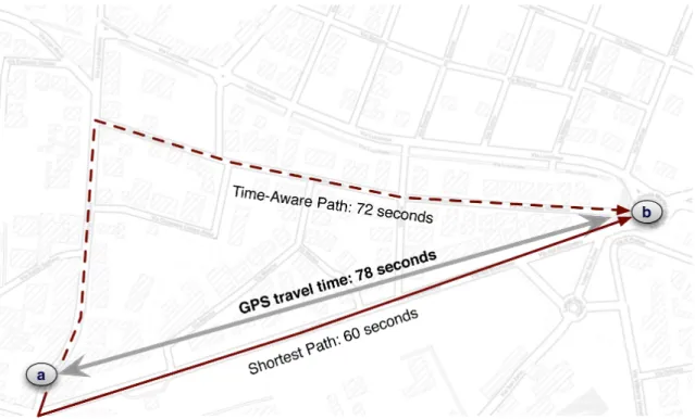
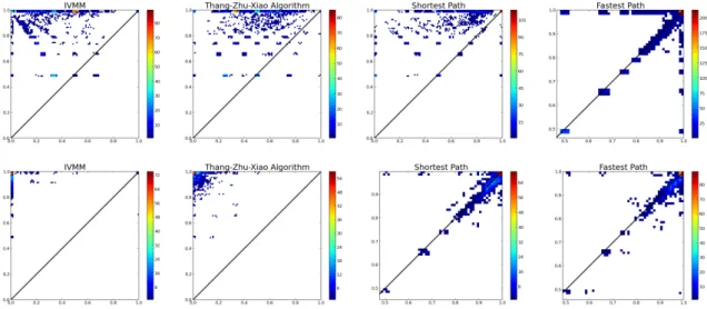
matching methods – we can actually check whether this happens or not. Figure 3.2 reports such an experiment; a shortest path method is applied to a real dataset of trajectories described in Section 3.7, and the travel time according to the algorithm is compared against the real one, obtained from GPS timestamps. It is clear that when the travel times become significant, larger than one minute, the reconstructed trips tend to be much faster than the real ones.

We propose an effective Time-Aware Map matching process for low-sampling rate GPS data based on the reduction of temporal mismatch introduced above. Fig. 3.1 provides the general workflow of Time-Aware map matching. With the initial and independent point-to-matching task we obtain a road network enriched with a precise time-dependent estimation of travel times (see upper part of the figure), based on the method proposed in 2. The core of our work is the second phase (lower part): a Time-Aware map matching algorithm that uses travel times to transform an input raw GPS trajectory -with travel time t- into a sequence of road segments with a travel time t0 ∼t.

In particular, we focus on finding the path between consecutive points that better fit the real travel time. Fig.3.3 shows the idea that guided us towards the develop-ment of this new approach. The raw GPS trajectory composed by points a and b has a travel time of 78 seconds. Once matched a and b to the corresponding road segments, thus obtaining source and destination of the path, there are two options: shortest path is also the fastest, with a travel time 60 seconds. An alternative path, there called Time-Aware, would be more reasonable to select, since it has a more similar travel times (72 seconds). The main contributions of this chapter can be

(50)

summarized as follows:

• a methodology for inferring speeds and traversal times of road segments is applied, based on the principles introduced in [18];

• a novel time-aware map matching method is proposed, that takes into consid-eration the real traversal times as described in the raw GPS data. A proof of the complexity of method is also provided, showing its higher scalability compared with existing competitors;

• a new methodology for evaluating the performances of map matching over large datasets, named middle point test, is introduced ad adopted;

• a wide comparison against the state-of-art competitors is performed, based on three real datasets: a small one from SigSpatial Cup 2012 and two large ones describing, respectively, the movements of taxis in San Francisco and private vehicles in Tuscany, Italy.

The outline of the chapter is as follows. Section 2 presents a survey of related works in the field of low-sampling rate map matching, while section 3 contains the definition of our proposed algorithm. Section 4 is dedicated to the validation of the algorithm, while in section 5 all the experiments on our dataset are reported. Section 6 gives the conclusion and introduces real applications and ideas for future works.

Figure 3.2: Average travel times of reconstructed path according to the GPS travel time of the original points. The area highlight the relative standard deviation. ∆ indicates the average difference between Path and GPS travel times.

Knowledge Discovery through Mobility Data Integration

Dipartimento di Informatica

Dottorato di Ricerca in Informatica

Ph.D. Thesis

Knowledge Discovery through Mobility

Data Integration

Paolo Cintia

Acknowledgments

Abstract

Contents

I

Background

17

II

Data integration: boosting the power of data

29

III

Conclusions, ongoing and future works

105

Introduction

Mobility Big Data

Part I

1

Related Works

1.1

The Map Matching Problem

1.2

Human Activities Recognition

1.3

Mobile Phone Data Knowledge Extraction

Part II

Data integration: boosting the

power of data

2

Exploiting GPS Data to assess

Road Network Travel times

2.1

Problem definition

2.1.1

The gravity model

2.1.2

Candidate selection

2.1.3

Buffer method

2.1.4

K-Neighbor method

2.2

From speed estimation to travel time

2.3

Validation

2.3.1

Generation of synthetic observations dataset

2.4

Performances study

2.5

Real case study

2.6

Summary

3

A Time Aware Map Matching

Method to enrich Raw

Spatio-Temporal Trajectories